Probabilistic program verification in the style of the unifying theories of programming

(1)

Riccardo Bresciani

Probabilistic Program Verification

in the Style of the

Unifying Theories of Programming

Ph.D. 2013

School of Computer Science and Statistics Trinity College Dublin

(2)

(3)

This thesis has not been submitted as an exercise for a degree at this or any other university. It is entirely the candidate’s own work. The candidate agrees that the Library may lend or copy the thesis upon request. This permission covers only single copies made for study purposes, subject to normal conditions of acknowledgement.

Riccardo Bresciani

(4)

(5)

To my wife, Chiara.

(6)

(7)

Summary

We present a novel framework to reason on programs based on probability distributions on the state space of a program: they are functions from program states to real numbers in the range

[0..1], which can be used to represent the probability of a program being in that state.

Such framework can be used to provide an elegant semantics in the style of UTPto a variety of programming languages using both probabilistic and nondeterministic constructs: the use of probability distributions allows us to give programs a semantics which is based on homogeneous relations.

The behaviour of probabilistic nondeterministic programs is treated algebraically via this frame-work, and as a result it is straightforward to derive algebraic expressions for the probability of some properties to hold for a given program.

Moreover our framework unifies all of the different kinds of choice under a single “generic choice” construct, and the usual choice constructs (disjunction, conditional choice, probabilis-tic choice, and nondeterminisprobabilis-tic choice) can be viewed as some of its specific instances. Later on we will discuss also other possible specific instances (namely conditional probabilistic choice, switching probabilistic choice, conditional nondeterministic choice, nondeterministic proba-bilistic choice, and fair nondeterministic choice).

The use of probability allows us to introduce the notion of probabilistic refinement, which generalises the traditional one: this is important in view of formal verification of probabilistic properties of programs via refinement-based techniques.

(8)

(9)

Acknowledgements

I wish to thank Andrew Butterfield and all of the guys from the FMG, without whom this work would not have been possible.

Obviously my friends and family have played a big part in this. Not long ago it took me a while to write up the acknowledgements for my master thesis, and now I would probably repeat the same things to the same people: for this reason allow me to simply condense my gratitude in a big thanks to you all.

The present work has emanated from research supported by Science Foundation Ireland grant 08/RFP/CMS1277 and, in part, by Science Foundation Ireland grant 03/CE2/I303_1 to Lero — the Irish Software Engineering Research Centre.

(10)

(11)

Introduction

Formal verification is now mainstream in computer science: the task of establishing if a given program behaves according to its specification is now a routine step, because of its higher reliability compared to tests, coupled with time- and money-saving possibilities deriving from a development approach based on formal methods.

The research community has played an important role in the development of current formal methods, and its effort has not stopped. As a result of all the different approaches adopted towards formal verification, nowadays we have a variety of available techniques: the advan-tage is that for each of the many verification scenarios a particular technique may prove more efficient than others.

On the other hand the disadvantage is interoperability of these techniques, which would be quite a desirable feature — it is absolutely standard to use several different techniques towards the verification of different parts of the same system.

Being able to use different models together is the aim of the Unifying Theories of Program-ming(UTP), which rely on predicate logic to give a semantics to different languages, so that unification can happen at the level of the common underlying semantics.

The focus of our work isUTP, in particular we want to come up with an approach that allows us to treat probabilistic programs in an analogous way as standard nondeterministic programs are treated inUTP.

There are several reasons for wanting probability in the picture.

A model including probability can offer a more precise description of a system, allowing the verification procedure to assert that a given propertyis verified with probabilityprather than simply asserting that the propertymay be verified.

An example is a system with two alternative behavioursAandB: if we knew nothing more than this, the only way we would be able to formalise is by merely saying that the system may show behavioursAandBbutwe cannot make any other kind of forecasts on the actual observable behaviour — we could write this using Dijkstra’s nondeterministic choice operator⊓asA⊓B. What if we had also some kind of statistical characterization of the system, for example thatA

andBhappen randomly half of the time? It would be an unnecessary and detrimental waste of information not to take this into account and model the system again with nondeterministic choice: a more desirable option is something saying that bothAandBhappen with probability

0.5— we could write something in the style ofA_0.5⊕B.

Sometimes a good statistical behaviour is what makes things usable. Actually, that is always the real-world case: any appliance or machine that we use is not guaranteed to work every time we want it to, it is just very likely that it will work.

Statistical observations are what draws a line between good appliances and bad ones: from

(16)

an observer’s perspective the functional difference between a Trabant and a BMW is based on statistics, one car being probabilistically less reliable than the other.

If we want to describe what happens when the driver turns the ignition key, simply saying that the engine may (or may not) start running is not a good enough description, a probabilistic information saying how likely it is that the car turns on is highly desirable.

We obviously have some expectations when we compare a Trabant with a BMW, as we assume that the components in one car are more reliable than the ones in the other car: we know that if we assemble correctly reliable components we will obtain a reliable car.

We have no numerical idea about the failure rate for the components used in each car, but an engineer does: from his perspective the observations on the behaviour of the car can be made at a lower level, directly on the parts, and this would allow him to infer the probability of some behaviour (assuming that there are no other design flaws).

This is another reason why it is interesting to talk about probability: the rules for deriving the probability of composite events from those of the single events are well established and understood. As a result the overall probability that a certain property holds in a system can be inferred bottom-up, starting from the probability of the relevant events.

An analogous perspective is that of the interaction between software and hardware: when we model the behaviour of a program the implicit underlying assumption is that the hardware is working properly. It would be interesting to integrate in the model also some information concerning possible hardware failures, which are to be characterised statistically.

An example is the use of flash memories: the physical principles they are based on are quite brutal (informally speaking, electrons are kicked through a barrier to store information, which can be then erased by a strong current flow that resets the whole memory block) so failures are of usual occurrence.

Having a framework which is capable to handle probabilistic information would be of great value here, for example each write operation to a flash memory could be rendered as:

write(x) ≙successful_write(x)_p⊕write_error

for an appropriatep, which can vary depending on number of previous writes and time.

From a different point of view, sometimes probability is the very reason why things do work. Miller-Rabin primality test is an example, and plenty of other examples of interest can be found in Computer Science, but also in everyday’s situations we rely on this: imperfect systems can be made more reliable through redundancy, both in terms of physical duplication of components and/or repetition of measures and experiments.

There are several pitfalls when dealing with probability, as sometimes the solution to some problems is quite confusing and counter-intuitive. Here are a few examples.

Think of a man who is the father of two children: • what is the probability that both of them are girls?

(17)

3

so obvious what the difference between the last two. Assuming that there is a 50% probability for each child to be male or female, the answers are:

• 1/_4;

• 1/_3;

• 1/_2.

The middle one is probably the most surprising answer.

This example highlights the subjective component of probability, as it varies depending on how well we know a situation we are talking about.

Another example is the (in)famous Monty Hall game: the setting is a TV show, where a par-ticipant in front of three closed doors is given the chance to win a car if he guesses the door, which the car has been hidden behind. Behind the doors there are two goats and a car, so the probability to choose the “right” door is1/_3.

But what if Monty Hall (the host) opens one of the remaining doors, thus revealing where one of the goat has been hidden, and offers the participant the possibility to change is mind and switch his choice to the other closed door? Should he do it?

The answer is yes, because in this way he will double his chances to win, jumping to a nice2/_3. This might sound a bit surprising at a first glance.

When trying to model a situation involving probability, the first and most important issue is the decomposition of such situation into events, distinguishing atomic events from composite ones. Atomic events are mutually independent, whereas composite events are a combination/union of atomic events.

For example if we pick a random natural number in the range[1..10]we can say that:

• the probability ofx=2is1/_10;

• the probability ofxbeing even is1/_2;

• the probability ofx=2andxbeing even is1/₁₀⋅1/₂=1/_20.

Or is it?!

The answer 1/₂₀ _{is wrong, because we have considered the two events “}_x = ₂_{” and “}_x _being even” as independent: in fact “xbeing even” is a composite event which can be rewritten in this case as “x=2orx=4orx=6orx=8orx=10” — after this observation it is clear thatxbeing even is always true whenx=2(i.e.the conditional probability ofxbeing even whenx=2is1), so the correct answer is1/_10.

Sometimes two events appear to be independent, but in reality there is a (possibly hidden) relation. A trivial example is a simple program that picks a random number forx(say either0

or1) and then assigns the new value ofxtoy.

Clearly the probability ofx =y is1, but would we be able to tell it if we were simply given

separatelythe probability distribution for each value for each variable, like:

(18)

In this case our answer would be probably that the probability is

P(x=0) ⋅ P(y=0) + P(x=1) ⋅ P(y=1) =1/₂_.

This is because we lost the “entanglement” between the variables that was created by the pro-gram.

1.1 Our approach

We want to give a brief overview of our approach, in order to give the reader an intuition without getting bogged down in details — which will be presented extensively in §3.

With the last example in mind, it is clear that if we want to give a probabilistic description of a program, we cannot deal with variables separately, but rather treat them as bundled into a single entity, which we call “state”.

Although the concept of state is very general, it can be thought of as a snapshot of the current memory content (what is in the RAM, in the processor registries, in the hard drive, and so on). Each state can be assigned a probability, which corresponds to the probability of the program being in that state: in this way we create a probability mass distribution, or shortly a proba-bility distribution, on the state space of a program, so that we can reason on the probability distribution (and its evolution) to understand the program behaviour.

Lumping variables together poses some serious challenges to track the evolution of a system: when a state evolves to another state, the associated probability (or a part thereof) has to be “transferred” to the new state. This is nontrivial in the case of several states evolving into the same state, so that the associated probabilities (or a part thereof) have to be summed together and “transferred” to the new state.

This is quite a common occurrence, for example this happens when there is an assignment operation.

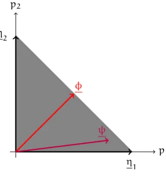
This framework has interesting algebraic properties, as the set of probability distributions is a precise part of a vector space made of more general distributions (i.e.those distributions that map states to real numbers, but that are not necessary a probability mass distribution), which is isomorphic to_Rn_{, with}_n_{equal to the number of states.}

Programs can consequently be seen asdistribution transformers: they take an initial distribution (before-distribution) and transform it into a final distribution (after-distribution) that accounts for the changes made by the program.

In the case of deterministic programs, the corresponding space has interesting properties as well, as it is isomorphic to a portion ofRn×Rn.

Nondeterminism arises when a program is entitled to choose internally between different al-ternative behaviours: as a result a single before-distribution can evolve to different possible after-distributions, all of which are equally valid and no forecasts on the actual outcome is possible.

(19)

1.1. Our approach 5

This allows us to see programs as predicates in the style ofUTP, which are based on homo-geneous relations among distributions: we are going to give a predicate semantics to a set of common constructs, and use this to reason on programs with the rules of predicate logic.

1.1.1 Key contributions

The key contributions of this work are:

• a novel framework to reason on programs based on probability distributions on the state space of a program: they are functions from program states to real numbers in the range

[0..1], which can be used to represent the probability of a program being in that state;

• such framework can be used to provide an elegant semantics in the style ofUTPto a vari-ety of programming languages using both probabilistic and nondeterministic constructs: the use of probability distributions allows us to give programs a semantics which is based on homogeneous relations. For this reason we believe that we took important steps to-wards. . .

. . . the so-far-unachieved goal of unifying probabilism with other program-ming constructs in the style of Unifying Theories of Programprogram-ming.

Chen and Sanders [CS09]

• such framework allows us to treat algebraically the behaviour of probabilistic nondeter-ministic programs, and as a result it is straightforward to derive algebraic expressions for the probability of some properties to hold for a given program;

• moreover our framework unifies all of the different kinds of choice under a single “generic choice” construct, and the usual choice constructs (disjunction, conditional choice, prob-abilistic choice, and nondeterministic choice) can be viewed as some of its specific in-stances. Later on we will discuss also other possible specific instances, namely:

– conditional probabilistic choice;

– switching probabilistic choice;

– conditional nondeterministic choice;

– nondeterministic probabilistic choice;

– fair nondeterministic choice.

• the use of probability allows us to introduce the notion of probabilistic refinement, which generalises the traditional one: this is important in view of formal verification of proba-bilistic properties of programs via refinement-based techniques.

1.1.2 Organization of this thesis

We are going to present the core background material which constitutes the foundations and main references for this thesis in §2.

(20)

from these chapters has been previously published as part of the work emanated from this research [BB09; BB11; BPB11; BB12a; BB12b; BB12c].

(21)

C

HAPTER

2

Background and related work

In this chapter we are going to present the background material relevant to this thesis and the related work; we assume familiarity with all of the underlying mathematics (linear algebra, measure theory and probability theory), which is anyway briefly presented in Appendix F. The topic of probability in computer science has been addressed within different scopes in a variety of different ways, including the Dempster-Shafer belief theory [Dem68; Sha76; Jøs01; Koh03], Bayesian networks [Pea88; FHM90], probabilistic argumentation [Hae+_{01], logical/relational}

Markov models [DK03; JKB07], and probabilistic powerdomain techniques [JP89; Jon90]. Our approach to probability builds on higher-level work relying on Markov models and prob-abilistic powerdomains, and in particular the main references are Dexter Kozen’s framework [Koz81; Koz85] and thepGCLframework [MM04]; such an approach yields aUTP-style frame-work where nondeterminism and probabilism coexist.

Kozen’s framework,pGCLandUTPare our three main reference areas: although the notation used in the different references varies, we will try to uniform it for the sake of understandability — refer to Appendix E for the notation used.

2.1 Kozen’s framework

In the early 1980s Dexter Kozen proposed a formalism to reason about probabilistic programs [Koz81; Koz85], with an approach which is very different from conventional logic:

Unfortunately, almost all of our logical apparatus belongs to the nondeter-ministic form. The usual logical connectives and the existential quantifier are clearly nondeterministic in nature. We must therefore be prepared to de-part radically from conventional logic in order to accommodate probability in a satisfactory way.

Kozen [Koz85]

Dijkstra’s nondeterministic choice is therefore left out in Kozen’s approach, and replaced by probabilistic choice: as we will see later on, this has profound implications.

The motivation for Kozen’s work was providing a common framework to unify the two main-stream approaches of the late 1970s, i.e. thedistributional approach and therandomized ap-proach, and to analyse probabilistic programs, which had been previously analysed exclusively byad hocmethods.

The distributional approach sees a program as being deterministic, and probabilism emerges from a probability distribution on the input; the randomized approach allows a program to

(22)

take probabilistic steps, but the input is fixed. Yao proved the equivalence of these approaches. [Yao77]

The roots of Kozen’s approach go down to the theory of linear operators in Banach spaces: a probabilistic program is in fact interpreted as a continuous linear operator on a Banach space of (probability) distributions.

Kozen deals withprobabilistic while programsin [Koz81], which act over the variables

_v

1,

v

2, . . . ,

v

n (all of the same type

_W

for the sake of simplicity) and use the following constructs:

_v

i∶=

random

, where

random

is a function returning a random variate from some random variable of the appropriate type1_;

• sequential composition:A;B, which executes the programBafterAhas terminated;

• conditional choice:A◁c▷B, which executesAorBdepending on the evaluation of the conditionc, which is a boolean expression2_;

• (while)loop:c∗A, which executes the body of the loopAas long ascholds true.

In semantics 1 of [Koz81] program variables are seen as random variables on the probability space(

_S

, Σ_S, µ_S), all of which have the same value space(

_W

, Σ_W), where:

• Σ_S = {α1, α2, . . .} ⊆ ℘

S

andΣ_W ⊆ ℘

W

areσ-algebras defined on the state space

S

and on the variable type

_W

;

• µ_S ∶Σ_S → [0..1]is a probability measure on the measurable space(

_S

, Σ_S).

We have that the functional composition of the probability measureµ_S after the random vari-able

_v

idefines a probability measure on(

W

, Σ_W):

µ_W ≙µ_S○

v

−1 i .

Therandom vector

_v

∶ (

_S

, Σ_S, µ_S) ↛ (

W

, Σ_W), where

_W

=

_W

n_and_Σ

W = {β1, β2, . . .} ⊆ ℘

W

, is a vectorial function whosei-th component is thei-th random variable; we can show that

_v

induces an isomorphism between the measurable spaces(

_S

, Σ_S)and(

_W

, Σ_W).

Similarly as above, the functional composition of the probability measureµ_S after the random vector

_v

defines the joint distribution for input variables:

µ_W ≙µ_S○

v

−1

.

1_{Kozen’s view of things in semantics 1 of [Koz81] is actually based on an infinite stack of random numbers, that}

serves as a random generator such that“each timevi∶=randomis executed, the next random number is popped from

the stack and assigned tovi”. The presentation of semantics 1 here is amended in order to avoid this complication:

it is possible to remove this by choosing to identify random vectors with the same distribution, according to Kozen’s observation at the end of the presentation of this semantics.

2_{A boolean expression}_c_{will evaluate to}_true_or_false_when_v_{is mapped to the to elements of a subset}_β

cofW or

toβ

¯

(23)

2.1. Kozen’s framework 9

A program Acan be seen as apartial measurable linear functionLA ∶

W

↛

W

on the value space, which accounts for the changes made byAto the configuration of variables; it is there-fore possible to express the joint distribution for the output we obtain after running programA

as:

µ′

W ≙µS○

v

−1○LA−1=µW ○LA−1.

In view of a slightly different semantics that appeared later in [Koz85] (and which is going to be presented below), it is useful to define now the probability measure

µ′

S≙µS○

Inv

A,

where

_Inv

A≙

v

−1○LA−1○

v

: the function

Inv

Aon(

S

, Σ_S)corresponds to the functionLA−1 on(

_W

, Σ_W)under the isomorphism induced by

_v

, and this implies that

µ′

W =µ

′

S○

v

−1.

Semantics 2 from [Koz81] sees a programAas a homeomorphism on the set of all possible joint distributions of the program variables (including all linear combinations), or equivalently as a homeomorphism HA on the setM_W of all possible probability measures on the measurable space(

_W

, Σ_W): therefore a program transforms a measureµ_W accounting for the initial vari-able distribution into a measureµ′

W =HA(µW)accounting for the final variable distribution

after the execution ofA— the notationAis used both for the program .

(M_W,∥ ∥,≤), where∥∥is the total variation norm and≤is the complete partial order induced by the positive coneM+

W ofMW, is aconditionally complete Banach lattice, where the internal

operations are defined as follows:

(µ_W_,i+µ_W_,j)(β) =µ_W_,i(β) +µ_W_,j(β)

(aµ_W)(β) =a(µ_W(β)).

The space

_P

of programs, with addition and scalar multiplication extended point-wise, forms

(24)

The intuition behind this approach is as follows. The program variables

v

1, . . . ,

v

n satisfy some joint distribution µ_W on input. We will forget the

variables themselves and concentrate on the distributionµ_W. We can think ofµ_W as a fluid mass distributed throughout

W

. This mass is concentrated more densely in some areas than others, depending on which inputs are more likely to occur. Execution of a simple or random assignment redistributes the mass in

_W

. Conditional tests cause the mass to split apart, and the two sides of the conditional are executed on the two pieces. In the while loop, the mass goes around and around the loop; at each cycle, the part of the mass which occupiesβ

¯

c breaks off and exits the loop, and the rest goes around

again. Part of the mass may go around infinitely often. Thus, at any point in time, there are different pieces of the mass that occupy different parts of the program, and each piece is spread throughout the domain according to the simple and random assignments that have occurred in its history. Different pieces that have come to occupy the same parts of the program through dif-ferent paths are accumulated. At certain points in time, parts of the mass find their way out of the program. The output distributionHA(µ_W)is the sum of all the pieces that eventually find their way out. Thus the probability that programAhalts on input distributionµisHA(µ_W)(

W

), the probability of the universal event

_W

upon output.

adapted fromKozen [Koz81]

Subprobability measures are all those positive ones whose norm does not exceed 1, which are those belonging to the setP≙M+

W∩ B0[1].

It shall be noted that, as probability measures are those with unitary norm,viz.belonging to the boundary∂B0(1)of the unit ball, the set of all positive probability measures is ˜P≙M+_W∩∂B0[1].

A program Acan therefore be seen as a function HA ∶→ P ↛ P, which maps a probability measure to a subprobability measure3_{. This function can be extended to be applicable on the}

v1

,

v2

, . . . ,

vn

) = (

v1

,

v2

, . . . ,

vi

−1, e(

v1

,

v2

, . . . ,

vn

),

vi

+1, . . . ,

vn

);

3_{Nevertheless more in general we can see them as a homeomorphism on the set of subprobability measures, as}

(25)

2.1. Kozen’s framework 11

• the random assignment

_vi

∶=

_random

H_random(µ_W)(β1×β2× ⋅ ⋅ ⋅ ×βn) =µ_W(β1×β2× ⋅ ⋅ ⋅ ×βi−1×

W

×βi+1× ⋅ ⋅ ⋅ ×βn)ρ(βi);

where β1, β2, . . . , βn ∈Σ_W andρis the probability distribution for the random number generator — the random assignment alters the measureβiused to have before its execu-tion, as the distribution of thei-th variable changes causingρ(βi)to be the new measure ofβi;

• the sequential compositionA;Byields the functional compositionHB○HA; • the conditional choiceA◁c▷Bis:

Hif(µ_W)(β) =HA○µ_W(β_c∩β) +HB○µ_W(β_c_¯∩β),

whereβcandβc¯are a partition of

W

: in these sets the conditioncevaluates to

true

and

false

respectively — it is therefore clear how the measure is transformed viaHA on the part ofβwherecis true and viaHBon the part ofβwherecis false;

• the loopc∗Acan be interpreted using theleast fixed pointoperator:

Hwhile(µ_W)(β) =lfpX(µ_W)(β) ● (X ○HA○µ_W(β_c∩β) +µ_W(β_c_¯∩β)),

where, in the right-hand side, a construct similar to the conditional choice is clearly recog-nisable: this is because the bracketed term was obtained by unfolding the loop once — the existence of the least fixed point is guaranteed by the fact that the space of programs

P

is a Banach lattice.

These ideas lead to the presentation in [Koz85], where programs are seen asMarkov transitions

(ormeasurable kernels), which are functionsp∶

S

×Σ_S →Rsatisfying the properties:

1. fα′(σ) ≙p(σ, α′)is a bounded measurable functionfα′∶

S

→Ron the measurable space (

S

, Σ_S)— letFdenote the space of all such functions;

2. µσ(α′) ≙p(σ, α′)is a finite measureµσ∶Σ_S →Ron(

S

, ΣS)— letMdenote the space of

all such functions.

The Markov transitionp(σ, α′)_{maps a pair, formed by a state and a set of states, to a real} num-ber: with an appropriate choice ofp, we can use a Markov transition to express the probability

pA(σ, α′)that a programAends up in some stateσ′∈α′when starting in stateσ.

With this in mind it is easy to relate this semantics to the measure-transformer semantics of [Koz81], by expressing the relation of a measure on the set of after-states

S

′_{to that on the set} of before-states

_S

as:

µ′

S(α′) = ∑

σ∈S

pA(σ, α′)µS({σ}).

It is also possible to use this to express the expected value ⟨f⟩ of a functionf ∶

S

′ →

R on

after-states after running a programAfrom a before-stateσ— therefore it is⟨f⟩ ∶

S

→R: ⟨f⟩(σ) = ∑

σ′∈S′

(26)

Iffis the characteristic function of a set of statesα′_{, then}⟨_f⟩_{is the probability that}_σ′∈_α′_{; if}

f is the function describing the probability of an event happening when a program halts in a given after-state, then⟨f⟩is the probability that this event happens when terminating in a state belonging toα′_.

A technique by Jones and Plotkin [JP89] can be used to build what they term theprobabilistic powerdomain of evaluations: they introduce probability into a semantic domain, and thus the behaviour described by Kozen’s framework can be reproduced in that setting [Jon90] — this is the basis for the probabilistic predicate-transformer model presented in §2.2 [MMS96; MM04].

2.2 pGCL

The choice operator is the key ingredient of probabilistic systems, and it can be instantiated in three different ways:

• demonic choice, that picks the “worst-case” scenario for that choice;

• angelic choice, that picks the “best-case” scenario for that choice;

• probabilistic choice, that picks one of the two options with a given probability.

Probabilistic choice is a desirable feature in a language, as it is doubtless that a quantitative formal analysis offers great advantages compared to a qualitative one: the challenge is to find a computationally feasible way of dealing with this.

Interactions among demonic, angelic and probabilistic choices may be subtle. In fact a deter-ministic (although probabilistic) program is characterised by monotonicity, conjunctivity and disjunctivity:

Monotonicity (P⇒Q) ⇒ (

P

(P) ⇒

P

(Q))

Conjunctivity

P

(P∧Q) ≡ (

When composing processes one must be careful about the issue ofduplication, which in pres-ence of probabilistic and nondeterministic choice may lead to incorrect results. [Mor+_95]

An example is given by the idempotency of the demonic choice operator, which depends on its definition: if the demonic choice operator can distribute through probabilistic choice operators we can have the following behaviour[Mis00]:

(A 1

2⊕

B) ⊓ (A1 2⊕

B) =A 1 4⊕ ((

A⊓B) 1 3⊕

B)

(27)

2.2. pGCL 13

Another way of seeing this is that it is crucial to know when a choice is made, thus we have to be very careful when we distribute choice operators.

The main shortcoming of Kozen’s approach is that he chooses not to retain nondeterministic choice, which — although being undoubtedly a source of complication — turns out to be a necessary and desirable feature of a programming language:

Dijkstra’s demonic⊓ was not so easily discarded, however. Far from being “an unnecessary and confusing complication,” it is the very basis of what is now known asrefinementandabstractionof programs.

McIver and Morgan [MM04]

In fact refinement and abstraction are the core of formal techniques for software specification and development, and are necessary to derive an implementation from a given specification via therefinement calculus.

Before going further on, let us take a step back and present the concept ofguarded commands, which was introduced by Dijkstra in the 1970s [Dij75; Dij76]: aguardis a condition that pre-cedes a command and is evaluated before the command is executed — obviously this happens only in case the guard is true.

TheGuarded Command Language(GCL) uses the following constructs:

•

_abort

is the aborting program;

•

_skip

is the program which does nothing and terminates;

• nondeterministic choice:A⊓B, which executesAorBnondeterministically, depending on the desired outcome — in the case of demonic nondeterminismthe executed program is that leading to the less desirable outcome, the one leading to the most desirable outcome in the case ofangelic nondeterminism;

In Dijkstra’s work, GCLis given a semantics via the so-called weakest precondition, which is a predicate

_wp

.A.

Post

that is true in thoseinitial statesthat guarantee that the postcondition

Post

will be reached after runningA4.

The work by Morgan, McIveret al.leads to a probabilistic version ofGCL, namelypGCL[MM97; MM04; MM05].

Our simple programming language will be Dijkstra’s, but with p⊕added and

— crucially — demonic choice⊓retained: we call itpGCL.

(28)

McIver and Morgan [MM04]

Their approach to probabilistic systems is based on what they termexpectations, which are used in place of standard predicates: informally, an expectation is a function that assigns aweight(a non-negative real number) to program states, thus describing how much each state is “worth” in relation to some desired outcome. This is nothing but a non-negative real-valuedrandom variable5.

There is a natural way of embedding the usual boolean predicates in this approach, as an expectation corresponding to a predicate

_Pred

can be defined as a random variable [

_Pred

] that maps a state to1if it satisfies the predicate and to0otherwise.

Arithmetic operators and relations are extended point-wise to expectations, as is multiplication by a scalar: the space of all expectations over the state space

_S

is

E = (

S

→R+,≤);

functions modifying an expectation are referred to asexpectation transformers.

pGCL is given a semantics based on expectations, which generalises the concept of weakest precondition to that ofweakest pre-expectation: for this reason this semantics is usually referred to as theweakest pre-expectation semantics— one expectation is weaker than another if for all states it returns at most the same weight (it is the≤relation lifted point-wise).

A pre-expectation is an expectation whose domain is that of initial states, whereas a post-expectation is an expectation whose domain is that of final states; given a post-expectation

PostE

and a program A, informally

_wp

.A.

PostE

is the weakest pre-expectation which de-scribes the expected “worth” of each initial state: the operator

_wp

can be thought of a function

wp

∶

P

→ T returning the expectation transformer corresponding to each program, whereT is the space of expectation transformers.

So we have that

PostE

∈ E and

wp

.A∈ T, and therefore

wp

.A.

PostE

∈ E. The syntax ofpGCLcomprises the following constructs:

•

_abort

is the aborting program;

•

skip

is the program which does nothing and terminates;

(1−p)— this is the novelty with respect toGCL;

• conditional choice:A◁c▷B, which executesAorBdepending on the evaluation of the conditionc— this is syntactic sugar forA

[c]⊕B;

• nondeterministic choice:A⊓B, which executesAorBnondeterministically;

5_{Attention must be paid to the terminology, which may be utterly misleading: many people refer to the expected}

(29)

≙

PostE

wp

.(c∗A).

PostE

≙lfpX●

wp

.((A;X) ◁c▷

skip

)

Figure 2.1:

_wp

-semantics ofpGCL, adapted from [MM04, p. 26].

Given a post-expectation

_PostE

, the weakest pre-expectation semantics corresponding to the constructs listed above is as follows:

• the weakest pre-expectation with respect to the aborting program is0regardless of

_PostE

:

wp

.

abort

.

PostE

=0;

• the program

_skip

does not alter the weight of each state, so the weakest pre-expectation is unchanged and therefore it is still

_PostE

:

);

• the weakest pre-expectation with respect to the probabilistic choice Ap⊕Bis a linear combination of the two alternative weakest pre-expectations with respect to Aand B, where the coefficientspand(1−p)respectively:

(30)

};

• in the case of the loop, the weakest pre-expectation can be determined via the least fix point operator in a standard way:

wp

.(c∗A).

_PostE

=lfpX●

_wp

.((A;X) ◁c▷

_skip

).

This is also shown in Figure 2.1.

Having retained nondeterminism, it is possible to define a sensible refinement relation using this semantics:

In other words a programArefines a specificationSif the minimum expected weight for each state afterAhas run is at least as much as we would get afterShas run.

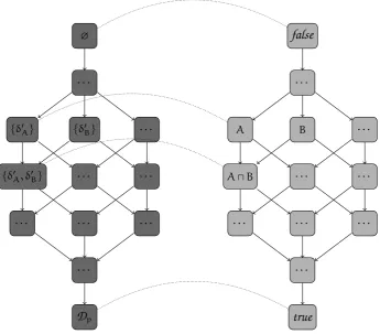
An alternative is theprobabilistic relational model[HSM97; MM04], which sees a program as a relation from states toup-, convex- and Cauchy-closed setsofprobability distributionsδover the state space — the characteristics of these sets correspond to some healthiness conditions on the probability distributions they contain, which will be discussed — ; the space of all probability distributions is

D

p= {δ∶

S

→ [0, 1] ∣ ∑σ∈S δ(σ) ≤1}.

It is possible to see programs as relations from probability distributions to sets of probability dis-tributions via theKleisli compositionof programs[MM04, Chp. 5] — incidentally, this is similar to our approach to givepGCLaUTPsemantics based on distributions.

From this perspective a probabilistic program is seen as a function that maps an initial state to a fixed final probability distribution over

_S

; the space of all deterministic programs is

P

D= (

S

→

D

p,⊑).

Because of nondeterminism each initial state can be mapped to different final probability distri-butions: it is therefore possible to see a demonic probabilistic program as taking an initial state to a set of fixed final probability distributions.

Such a set cannot be any subset of

_D

p, as the distributions it contains must comply with some healthiness criteria, as mentioned above: this results in the set being up-, convex- and Cauchy-closed.

The space of all demonic probabilistic programs is therefore

(31)

2.2. pGCL 17

Theprobabilistic predicate-transformer modeltakes a program and turns it into an expectation transformer. This can be applied to a post-expectation to derive the corresponding pre-expectation.

pre-expectation

E

expectation transformer

T

post-expectation

E

program

wp

The probabilistic relational model relates a state to an up-, convex- and Cauchy-closed set of probability sub-distributions.

state

S

program

P

up-, convex- and Cauchy-closed set of probability sub-distributions

[image:31.595.145.493.101.293.2]

C

Figure 2.2: The two semantic models ofpGCLfrom [MM04].

whereH ⊆ ℘

_D

pis the set of all up-, convex- and Cauchy-closed sets of probability distributions; these three set properties descend from healthiness conditions that are satisfied only by those distributions that result from sensible probabilistic programs:

Probabilistic programs are now modelled as the set of functions from ini-tial state in

_S

to sets of final distributions over

_S

, where the result sets are restricted by so-called healthiness conditions characterising viable proba-bilistic behaviour, motivated in detail elsewhere [MM04]. By doing so the semantics accounts for specific features of probabilistic programs. In this case we impose up-closure(the inclusion of all⊑-dominating distributions),

convex closure(the inclusion of all convex combinations of distributions), and Cauchy closure(the inclusion of all limits of distributions according to the standard Cauchy metric on real-valued functions [MMS96]). Thus, by construction, viable computations are those in which miracles dominate (re-fine) all other behaviours (implied by up-closure), nondeterministic choice is refined by probabilistic choice (implied by convex closure), and classic limiting behaviour of probabilistic events (such as so-called “zero-one laws”) is also accounted for (implied by Cauchy closure). A further bonus is that (as usual) program refinement is simply defined as reverse set inclusion. We observe that probabilistic properties are preserved with increase in this order.

adapted fromMcIver, Cohen, and Morgan [MCM06]

The visual synthesis of the semantic models is presented in Figure 2.2.

(32)

To conclude this brief presentation of pGCL, here is a representative sample of laws about probabilistic programs, that it is possible to prove in this framework:

A⊓B⊑A_p⊕B

(A⊓B)_p⊕C= (A_p⊕C) ⊓ (B_p⊕C)

(A⊓C)_p⊕ (B⊓C) ⊑ (A_p⊕B) ⊓C

(A⊓B);C= (A;C) ⊓ (B;C) A;(B⊓C) ⊑ (A;B) ⊓ (A;C)

2.3 pCSP

On the side of process algebras, probabilistic CSP is obtained by adding probability to Hoare’s CSP [Hoa85b].

In [Mor+_{96] we can find one of the possible definitions, where probability is defined in such a}

way that it distributes through all operators: this leads to a surprising behaviour in the demonic choice operator, which is not idempotent.

In this paper they define a refinement operator and discuss the ideas of an associated probabilis-tic refinement calculus, where an implementation satisfies a specification with null probability: this shows that it is not reasonable to expect an absolute specification in this setting, but it is wiser to have a sort of “timed” specification. This is in line with real-world systems, as they cannot possibly work forever (we simply have to wait long enough for their failure probability to raise), and for this reason we can specify a time limit for which a specification has to be satisfied.

A different presentation is given in [Mor04], wherepCSPis built on top of probabilistic action systems written inpGCLand is linked back to the relational semantics ofpGCL.

This view of the subject highlights how compositionality of probabilistic CSP is not straight-forward, because of the introduction of probability: in a way probability splits the deterministic scenario into several possible different scenarios, and one has to take this into account when composing probabilistic programs.

They explain this using the metaphor of the colour of a child’s eye, knowing the colour of the parents’ — too much information has to be brought forward if we want accurate information, but simply a phenotypical description is unreliable and not sufficient, as what is enough is to know colour and whether the allele is predominant or recessive. This same kind of information is the one that has to be sought to have an accurate probabilistic compositionality: in fact if we observe an event, we would want to be able to identify the facts that have led to that event. For example if we observe a failure (i.e. a composite event) during the run of a program, we want to track down the reasons of this failure and to identify what factors (i.e. base events) have been responsible for the happening.

2.4 UTP

(33)

2.4. UTP 19

Computing science is a new subject, and we have not yet achieved the unifi-cation of theories that should support a proper understanding of its structure. [. . . ] we face the challenge of building a coherent structure for the intel-lectual discipline of computing science, and in particular for the theory of programming. Such a comprehensive theory must include a convincing ap-proach to the study of the range of languages in which computer programs may be expressed. It must introduce basic concepts and properties which are common to the whole range of programming methods and languages. Then it must deal separately with the additions and variations which are particular to specific groups of related programming languages.

Hoare and He [HH98]

A success in this area has been the development of theCircus language [OCW09], which is a fusion of Z and CSP, with aUTPsemantics, providing specifications using a “state-rich” process algebra along with a refinement calculus; recent extensions to Circus have included timed [SH03] and synchronous [GB09] variants. Recent interest in aspects of the POSIX filestore case study in the Verification Grand Challenge [FWB08] has led us to consider integrating probability intoUTP, with a view to eventually having a probabilistic variant ofCircus.

UTPfollows the key principle that “programs are predicates” [Heh84; Hoa85a] and so does not distinguish between the syntax of some language and its semantics as alphabetised predicates; theories inUTPare expressed as second-order predicates6over a pre-defined collection of free

observation variables, referred to as thealphabetof the theory. The predicates are generally used to describe a relation between a before-state and an after-state, the latter typically characterised by dashed versions of the observation variables. For example, a program using two variablesx

andymight be characterised by having the set{x, x′_{, y, y}′}_{as an alphabet, and the meaning of} the assignmentx∶=y+4would be described by the predicate

x′=

y+4∧y′=

y.

In effectUTP uses predicate calculus in a disciplined way to build up a relational calculus for reasoning about programs.

In addition to observations of the values of program variables, often we need to introduce observations of other aspects of program execution via so-called auxiliary variables. So, for example, in order to reason about total correctness, we need to introduce boolean observa-tions that record the starting (

_ok

) and termination (

_ok

′) of a program, resulting in the above assignment having the following semantics:

ok

⇒

ok

′

∧x′=

y+4 ∧y′=

y

(if started, it will terminate, and the final value ofxwill equal the initial value ofyplus four, withyunchanged).

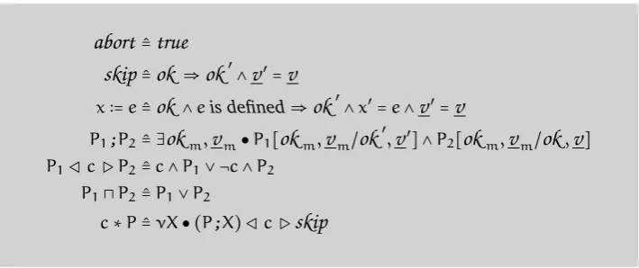
As an example of aUTPtheory using both observation and auxiliary variables, we have shown in Figure 2.3 the UTP semantics of a variant of Dikstra’s GCL [Dij76] according to the so-called theory of “designs”, which characterises total correctness for imperative programs.xis a

6_{Most definitions are in fact first-order, but we need second-order in order to handle the notion of “healthiness”,}

(34)

abort

≙

true

skip

≙

ok

⇒

ok

′

v

′] ∧

P2[

ok

m,

v

m/

ok

,

v

]

P1◁c▷P2≙c∧P1∨ ¬c∧P2

P1⊓P2≙P1∨P2

[image:34.595.98.453.83.232.2]

c∗P≙νX● (P;X) ◁c▷

skip

Figure 2.3: UTPDesign semantics of simplifiedGCL

program variable and

v

is the list of all other program variables, and thus these are observation variables, and

_ok

is an auxiliary variable.

A problem with allowing arbitrary predicate calculus statements to give semantics is that it is possible to write unhelpful predicates such as ¬ok ⇒ ok′_{, which describes a “program” that} must terminate when not started. In order to avoid assertions that are either nonsense or infeasible, UTP adopts the notion of healthiness conditions which are monotonic idempotent predicate transformers whose fixpoints characterise sensible (healthy) predicates. Collections of healthy predicates typically form a sub-lattice of the original predicate lattice under the reverse implication ordering [HH98, Chapter 3].

Key inUTPis a general notion of program refinement as the universal closure of reverse impli-cation7_:

m●

P

{vm/v}

(35)

2.4. UTP 21

Which reduces to

_true

if

_v

∈

_fv

(

_P

), or to

_P

otherwise.

This has disastrous consequences, as this enables us to show that a program can recover from a never-ending loop:

true

∗

skip

≡lfpX●X≡ ≡

true

⇒

ok

′

∧

Post

≡∃

ok

m,

v

m●

true

{okm/ok′}{vm/v′} ∧ (

ok

_m∧

Pre

{vm/v} ⇒

ok

′

∧

Post

)

′

∧

Post

)

Post

≡

true

and therefore

_true

ok

It should be noted that

_miracle

is a (infeasible) program that cannot be started.

Valid designs are predicatesRwhich comply with four healthiness conditions [HH98]. The first one (unpredictability, H1) excludes from observation all programs that have not started, and therefore restricts valid relations to those such that:

(36)

AllH1-healthy predicates satisfy the left zero and left unit laws:

true

;R=

true

and

_skip

;R=R

The second one (possible termination,H2) states that a valid relation cannot require nontermi-nation:

R{false_/_ok′_{} ⇒}_R_{_true_/_ok′_}

The third one (dischargeable assumptions,H3) states that preconditions cannot use dashed vari-ables. AllH3-healthy predicates satisfy the right unit law:

R;

skip

=R

The fourth one (feasibilityorexcluded miracle,H4) requires the existence of final values for the dashed variables that satisfy the relation:

∃

ok

′

There has already been a certain amount of work looking at encoding probability in a UTP

setting. He and Sanders have presented an approach unifying probabilistic choice with stan-dard constructs [HS06], and this work provides an example of how the laws ofpGCLcould be captured inUTP as predicates about program equivalence and refinement. However only an axiomatic semantics was presented, and the laws were justified via a Galois connection to an expectation-based semantic model.

Sanders and Chen then explored an approach that decomposed demonic choice into a combi-nation of pure probabilistic choice and a unary operator that accounted for demonic behaviour [CS09]. There they commented on the lack of a satisfactory UTP theory which could prove effective towards. . .

. . . the so-far-unachieved goal of unifying probabilism with other program-ming constructs in the style of Unifying Theories of Programprogram-ming.

Chen and Sanders [CS09]

A probabilistic BPEL-like language has recently been described by He [He10] that gives aUTP

(37)

2.4. UTP 23

an initial state and a final probability distribution over states.

In relatively recent times a paper by Jun Sunet al.[SSL10] has described a probabilistic anal-ysis of the likelihood of a program in a medical device satisfying a safety specification, given that random, but hopefully unlikely events, can prevent the correct behaviour, even if the pro-gram is the best one possible. Their probabilistic model checking directly corresponds to the probabilistic refinement we are going to present in §3.7.1.

What all the treatments above have in common is that the UTP predicates relate an initial program variable state (σ) to a final probability distribution (δ′_{) over states, so the relation} is not homogeneous. This complicates the definition of sequential composition (which has to involve some form of Kleisli composition) and also makes building links to homogeneousUTP

theories more difficult.

What is still missing is aUTPtheory that is defined in terms of predicates based on before/after relations over thesameobservation space.

SeveralUTPtheories are based on homogeneous relations: this means that all of these theories have uniform definitions of many common language features, such as sequential composition. For example the collection of theories surroundingCircusare all uniform, so the development of a homogeneous probabilisticUTPtheory would open way towards a reasonably easy devel-opment of a probabilistic theory ofCircus.

(38)

(39)

C

HAPTER

3

A framework to deal with

probability distributions over the

state space

This chapter is dedicated to a quite detailed presentation of the framework we have developed: we have decided to privilege clarity of the exposition over pedantic details, which are therefore presented in the appendices along with many of the proofs for properties and theorems. The fundamental reason why we felt the need of a different framework is that the existing ones do not integrate very well in theUTP framework, in the sense that dealing with probability is dealing with a great amount of information and complex constructs at a very low level. In particular one of the key strengths of our framework is the use of homogeneous relations among distributions on the state space to model programs: in previous work the approach was to relate a single state to a distribution on the state space, which contains information on the probability of the different resulting states. The non-homogeneity of this relation makes sequential composition a non-trivial matter.

Also, in order not to get bogged down in unnecessary details, much of the complexity under is hidden under the hood, so that we can reason (quite) smoothly on probabilistic programs at a higher level.

These features together allow us to deal in a straightforward way with both nondeterminis-tic and probabilisnondeterminis-tic choice: we deem this to be an important step towards the development of general probabilistic theories of a variety of languages already treatable in UTP in their non-probabilistic version, such as CSPor Circus, as we believe it helps overcome the current unsatisfactory approaches bringing probabilism and nondeterminism together [CS09].

Coherently with theUTPapproach, programs are captured as predicates with a suitable alpha-bet.

Hehner and Hoare wrote that “programs are predicates” [Heh84; Hoa85a], we affirm that

probabilisticprograms are predicates too.

3.1 States and distributions, informally

Before presenting formally the foundations of our framework, we find it useful to give a gen-eral and intuitive overview, where we sacrifice formality and rigour in favour of a more relaxed introduction of the basic concepts: this should allow the reader to have an intuitive under-standing of the key points, which we are going to introduce formally in the remainder of the chapter.

(40)

UTPpredicates usually involve relations between variables from the predicate alphabet and the corresponding values: some people feel that a tempting approach may be to try a naïve (and quite straightforward) generalization of this standard situation by relating a variable to a pair containing its possible value and the corresponding probability.

In this case the idea is to deal with objects with the following shape1_:

V

→ (

W

→ [0..1]),

where

_V

and

_W

are appropriate sets of program variables and corresponding values, respec-tively.

It should be quite evident that this is not a satisfactory approach. At the risk of stating the obvious, the reason is that this approach takes each variable individually, so it assumes the independence of the value assumed by each variable from that of any other — and this is clearly an assumption which is wrong in general.

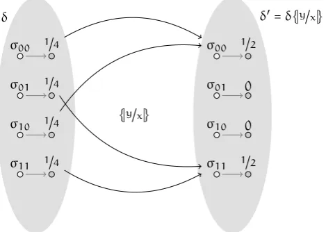
To see this let us consider an example, where a program with variables x, y starts in a state wherexandyare each independently initialized to0with probability1/₂_{and to}₁_with prob-ability1/_{2. This program consists simply in the assignment}_x∶=_y_{and so the situation after the} program has run can be described as follows, with obvious meaning of the notation:

x↦⎛

⎝

0↦1/₂

1↦1/₂

⎞

⎠, y↦

⎛ ⎝

0↦1/₂

1↦1/₂

⎞ ⎠.

The information contained in this description is incomplete, as it does not tell us anything about the relation between the variables; in this case it seems we are able to make predictions on the expected value of each variable taken separately2 (e.g.the probability ofx =1 is 1_/₂_{), but as}

soon as we try to reason on a more complex event, such as the probability ofx=y, things go terribly wrong. If we crudely look at the numbers, the probability we are looking for is:

P(x=y) = P(x=0) ⋅ P(y=0) + P(x=1) ⋅ P(y=1) =1/₂_.

This is quite an upsetting “I-told-you-so” result, as all the program did was to assign the value ofytox, so we would have expectedP(x=y) =1.

So, although such an easy generalization may (?) look appealing, this example clearly shows how this is not a viable approach, as it loses theentanglementamong the variables.

A better approach should rather use objects with this other shape:

(

V

→

W

) → [0..1].

The example above with this different approach gives the following description:

⎛ ⎝

x↦0 y↦0

⎞ ⎠↦1/2,

⎛ ⎝

x↦1 y↦1

⎞ ⎠↦1/2.

This approach assigns different probability to the different mappings σ∶

V

→

W

that relate

1_{We underline whenever we talk about vectors or sets of vectors:}_A_{stands for a}_n_{-th dimensional vectorial space}

A×A× ⋅ ⋅ ⋅ ×A, for an appropriaten.

Probabilistic program verification in the style of the unifying theories of programming

Riccardo Bresciani