Manuscript version: Author’s Accepted Manuscript
The version presented in WRAP is the author’s accepted manuscript and may differ from the published version or Version of Record.
Persistent WRAP URL:
http://wrap.warwick.ac.uk/122988
How to cite:
Please refer to published version for the most recent bibliographic citation information. If a published version is known of, the repository item page linked to above, will contain details on accessing it.
Copyright and reuse:
The Warwick Research Archive Portal (WRAP) makes this work by researchers of the University of Warwick available open access under the following conditions.
Copyright © and all moral rights to the version of the paper presented here belong to the individual author(s) and/or other copyright owners. To the extent reasonable and
practicable the material made available in WRAP has been checked for eligibility before being made available.
Copies of full items can be used for personal research or study, educational, or not-for-profit purposes without prior permission or charge. Provided that the authors, title and full
bibliographic details are credited, a hyperlink and/or URL is given for the original metadata page and the content is not changed in any way.
Publisher’s statement:
Please refer to the repository item page, publisher’s statement section, for further information.
Effective mean free path and viscosity of confined gases
Jianfei Xie,1,a) Matthew K. Borg,2,b) Livio Gibelli,2,c) Oliver Henrich,3,d)
Duncan A. Lockerby,4,e) and Jason M. Reese2,f)
1)School of Engineering, University of Derby, Derby, DE22 1GB,
UK
2)School of Engineering, University of Edinburgh, Edinburgh, EH9 3FB,
UK
3)Department of Physics, University of Strathclyde, Glasgow, G4 0NG,
UK
4)School of Engineering, University of Warwick, Coventry, CV4 7AL,
UK
(Dated: 13 June 2019)
The molecular mean free path (MFP) of gases in confined geometries is numerically
eval-uated by means of the direct simulation Monte Carlo (DSMC) method and molecular
dynamics (MD) simulations. Our results show that if calculations take into account not
only intermolecular interactions between gas molecules, but also collisions between gas
molecules and wall atoms, then a space-dependent MFP is obtained. The latter, in turn,
per-mits one to define an effective viscosity of confined gases that also varies spatially. Both the
gas MFP and viscosity variation in surface-confined systems have been questioned in the
past. In this work we demonstrate that this effective viscosity derived from our MFP
calcu-lations is consistent with those deduced from the linear-response recalcu-lationship between the
shear stress and strain rate using independent non-equilibrium Couette-style simulations,
as well as the equilibrium Green-Kubo predictions.
Keywords: rarefied gas; mean free path; near-wall viscosity; direct simulation Monte
Carlo; molecular dynamics
a)Electronic mail: [email protected]
b)Electronic mail: [email protected];corresponding author
c)Electronic mail: [email protected].
d)Electronic mail: [email protected]
e)Electronic mail: [email protected]
I. INTRODUCTION
Rarefied gas flows are of ongoing interest, because of their fundamental nature and many
ap-plications in different fields including aerodynamics and heat transfer29,44,
micro/nano-electro-mechanical systems (MEMS/NEMS)12, and shale gas recovery14,41. The traditional
dimension-less measure of the degree of rarefaction is the Knudsen number (Kn), defined as the ratio of the
molecular mean free path (MFP) to the characteristic dimension of the gas flow.
Rarefaction effects cause gas flows to deviate from continuum fluid behaviour when Kn&10−3.
More specifically, for moderate Knudsen numbers in the slip flow regime (10−3.Kn.10−1),
these effects are confined to thin layers close to the bounding surfaces, which are referred to as
Knudsen layers. These layers may be accounted for in the conventional Navier-Stokes
descrip-tion with slip/jump boundary condidescrip-tions for the velocity and temperature12. In the transition flow
regime (0.1.Kn.1), rarefaction effects become appreciable in the whole domain, and, in
prin-ciple, the accurate description of a gas flow requires the solution of the Boltzmann equation or
simplified kinetic model equations12. Thermodynamic non-equilibrium gas flows are met in
dif-ferent physical situations ranging from low pressure conditions in the upper regions of planetary
atmospheres (i.e. low-density gas flows in near-vacuum environments) to high pressure conditions
in very small channels (i.e. dense gas flows in micro/nano confinements).
Solving gas kinetic equations, either by the stochastic direct simulation Monte Carlo (DSMC)
technique8, or by deterministic methods4,16, such as molecular dynamics (MD), is computationally
demanding, especially for flows that are three-dimensional and/or involve both continuum and
rarefied regions35. Therefore, much effort has been done over the years to extend the continuum
fluid dynamics description to the transition regime. A first approach to incorporating rarefaction
effects into a continuum description relies on the higher-order continuum equations that are derived
from the kinetic equations via the Chapman-Enskog series solution technique, the Grad moment
method, or a combination of these two37. A second and simpler approach consists in using an
effective viscositywith the original strain-rate in the linear constitutive relationship of the
Navier-Stokes equations, i.e.
µeff(z) = 1
Ψ(z)µ0, (1) whereµ0is the nominal viscosity of the gas, andΨ(z)is an expression of the high-order non-linear correction terms, which depends on the normal distance z to the nearest solid wall22,24–27. The
effects can be disregarded, i.e.,Ψ(z)→1 asz→∞in Eq. (1).
The simplest way to define an effective viscosity is to use the direct proportionality between
viscosity and the molecular mean free path (MFP) as predicted by elementary kinetic theory
argu-ments in equilibriumconditions13,23. Accordingly, this produces a high-order non-linear
correc-tion term as follows:
Ψ(z) = λ0
λeff(z), (2)
whereλ0is the nominal MFP in the space-homogeneous conditions, andλeffis theeffectiveMFP
of gas molecules in confined geometries. The nominal MFP for hard-sphere molecules is
rigor-ously defined as:
λ0,h=
m
√
2πd2ρ
, (3)
while for molecules interacting through long-range potentials, it can be qualitatively expressed
as12:
λ0,v= µ0
ρ
r
πm
2kBT
. (4)
In Eqs. (3) and (4),ρ is the gas density,mis the molecular mass,dis the molecular diameter,T is
the temperature of the gas, andkB is the Boltzmann constant.
Stops36 first derived a space-dependent expression for λeff of gas molecules leaving a wall,
distributed according to the diffusive Lambert’s cosine law of reflection. Several decades later,
Guo et al.20 extended the Stops’ model to propose the MFP of confined gases as:
λeff,G(z)
λ0
=1−1
2
z2E1(z) + (1−z)e−z, (5)
whereE1(z)is the exponential integral function, i.e.E1(z) =Rz∞e−z/zdz. More recently, Abramov1,2
has introduced a new expression for the MFP of gases in confined geometries by replacing the
cosine law with the equilibrium Maxwellian to give:
λeff,A(z)
λ0
=1−1
2
e−z−yE1(z). (6)
Beside theoretical research in this area, there have been a number of recent studies in which
molecular dynamics (MD) simulations have been used to directly evaluate the MFP in a gas by
averaging the recorded individual free paths5,7,17,31,39. However, there is still debate about the
behaviour of the effective MFP in confined geometries, and whether this is physical or not. Some
studies take into account the collisions between the freely moving gas molecules and wall atoms,
Others7 have argued that the collisions between the freely moving gas molecules and solid wall
atoms (or gas molecules adsorbed on the walls) should be disregarded when evaluating the
indi-vidual free paths. The latter study shows that the MFP should not vary spatially and conclude that
the effective viscosity provided by Eq. (1) is questionable7.
The main aim of the present paper is to resolve disputes in the literature about the spatial
vari-ation of the MFP for gases in confined geometries, such as in flows through micro/nanochannels.
For this purpose, the MFP is computed numerically now by means of both DSMC and MD on the
basis of its definition, namely by averaging the distance travelled by molecules between two
con-secutive collisions. Our aim is also to demonstrate using different techniques for measurements of
viscosity that thereisa variation in viscosity near a surface, thereby validating Eq. (1).
It is the first time that DSMC has been used for this kind of investigation until now. The DSMC
technique offers a number of advantages compared to MD simulations, such as the computational
efficiency and the possibility to more easily assess the theoretical predictions proposed in the
literature2,20. On the other hand, MD remains the key simulation tool in that, in principle, it
enables the study of more complex and realistic fluid flows14,43, including the important
gas-surface interactions.
The rest of the paper is organised as follows. In Section II, we briefly present the DSMC and
MD approaches, and we discuss the procedure for the direct determination of the MFP. In
Sec-tion III, we first investigate how the MFP of gas molecules is modified when their dynamics are
constrained by a confining geometry and we assess the accuracy of the theoretical predictions
pro-posed so far, i.e. Eqs. (5) and (6) (Subsection III A). We then measure viscosity using independent
methods and compare our results with Eq. (1) in Subsection III B. Conclusions and future work
are then drawn in Section IV.
II. EVALUATION OF MOLECULAR MEAN FREE PATHS
A. Direct simulation Monte Carlo
The DSMC technique was initially introduced for gas simulations based on physical
argu-ments8, but it has been proved to converge, in a suitable limit, to the solution of the Boltzmann
equation40. The basic idea of DSMC consists in representing the velocity distribution function
cell
(a) DSMC (b) MD
collision
fre e flight
,
collision
fre e flight
,
collision
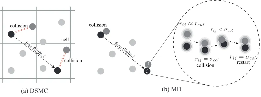
[image:6.612.83.534.72.240.2]collision restart
FIG. 1: Schematic of the calculation of individual free paths in our (a) direct simulation Monte
Carlo and (b) Molecular Dynamics simulations.
are decoupled over a time step ∆t, which is smaller than the average collision time. The space domain to be simulated is divided into a mesh of cells whose size∆zis less than the MFP. These cells are used to collect together particles that may collide according to stochastic rules derived
from the Boltzmann equation. The cells employed for simulating interactions are also used for the
sampling of macroscopic properties, which are obtained through weighted averages of the particle
properties.
In the present work, particles’ collisions are evaluated based on the hard sphere molecular
model, which provides a reliable description of isothermal gas flows of argon-like molecules. The
particles’ free paths are evaluated by tagging particles and keeping track of their free flight distance
by an appropriate counter that measures the distance incremented by a particle in each time step, as
shown in Fig. 1(a). The free path is therefore a sum over all displacements between two successive
collisions:
li(z) = n
∑
j=1
vi,j∆t, (7)
where vi,j is the speed of the ith particle at timetj, n is the number of time steps between two
successive collisions,z is the coordinate of the bin where the particle collided, and ∆t is the nu-merical time step. Note that if external force fields are absent, such as in the case of DSMC, the
particle’s velocity between two consecutive collisions is constant and, therefore, it can be taken
out of the sum. When a particle collides, the free path is terminated, and the counter is set to zero
whether the collision occurred with a wall or with another particle. As particle-particle collisions
post-processing.
The mean free path is then easily obtained by averaging over particles:
λ(z) = N
∑
i=1
li(z)
N(z) , (8)
whereN(z)is the total number of particles that have terminated their free path in the bin of
coor-dinatez. Our numerical experiments have shown that the MFP is discontinuous if the free flights
of the molecules hitting the walls are attributed to the cells closest to them. The continuity of the
MFP is recovered by setting to zero the counter of molecules which suffer a collision with walls,
but disregarding their free flight contribution.
The DSMC simulations we report below have been obtained with ∆z= 10−2λ0 and ∆t =
2×10⁻³t0, wheret0 =λ0/(kBT0/m), andλ0 and T0 are the nominal mean free path and a
ref-erence temperature, respectively. Computational particles are initially distributed according to a
Maxwellian at the temperature T0 and their average number per cell during simulations is about
102. The evolution of the system is simulated for 103t0. As an input parameter for the
bound-ary condition, both fully diffusive wall, i.e. the tangential momentum accommodation coefficient
(TMAC)α =1.0, and a mixture of partially diffusive and partially specular walls (i.e. α <1.0)
have been used in our DSMC simulations: four values of the TMAC (i.e.α=0.2, 0.4, 0.6, 0.8 and
1.0) are tested. Our results show that the influence of the TMAC on the calculations of MFP is
neg-ligible. For the sake of simplicity, the fully diffusive wall is adopted in all our DSMC simulations
below.
B. Molecular dynamics
In MD simulations, the molecules move according to Newton’s second law, and the
inter-molecular interactions are modelled through a prescribed interatomic potential. In the present
study, monatomic argon (Ar) gas is used and it is assumed that molecules interact through the
Lennard-Jones (LJ) potential:
ULJ ri j=
4ε " σ
ri j
12 −
σ
ri j
6#
, ri j≤rc,
0, ri j>rc,
TABLE I: Physical parameters and their values in our MD simulations. SubscriptsArandPt
refer to argon and platinum atoms, respectively, andkBis the Boltzmann constant.
Parameter Symbol Value
Length scale σAr 3.405×10⁻¹⁰[m]
σAr−Pt 3.085×10⁻¹⁰[m] Energy scale εAr 1.67×10⁻²¹[J]
εAr−Pt 0.894×10⁻²¹[J] Molecule mass mAr 6.63×10⁻²⁶[kg]
mPt 3.24×10⁻²⁵[kg]
Time scale τ=σAr
q
mAr
εA 2.15×10⁻¹²[s] Temperature εAr/kB 119.8 [K]
whereri j is the intermolecular distance, ε is the energy parameter,σ is the molecular diameter,
andrc is the cutoff distance.
For the measurement of individual free paths, as shown in Fig. 1(b), a condition is set to
judge the occurrence of a collision event between gas molecules: if the distance between two
gas molecules is equal to or less than the collision diameterσcol, i.e.ri j ≤σcol, the two molecules
have collided and we stop recording the free paths of the involved molecules. We describe the
procedure used to define the collision diameter in our MD simulations, in Appendix A.
As the LJ potential allows any pair of molecules to move closer to each other, even whenri j<
σcol, then the finite time spent during this collision process must be excluded when calculating the
individual free paths. Therefore, we restart recording the free paths when the distance between
the molecules is again larger than the collision diameter, i.e. whenri j >σcol. In this procedure,
the counter for recording each molecular free path is switched on after the last collision between
two molecules and it is not switched off until the next collision. We also count collisions between
gas molecules and wall atoms: if the gas molecule approaches a wall and crosses a virtualplane
that is placed σcol away from and parallel to the wall, we say it has collided with the wall and
stop recording its free path. The MFP is computed using the same equations in the DSMC setup,
two consecutive collisions because of the long range nature of the Lennard-Jones potential.
The open source code LAMMPS32 is used to perform our MD simulations reported below, and
a new class has been developed to calculate the individual molecular free paths. The potential
is truncated at a cutoff of rc =2.5σAr, and the neighbour list method is adopted to reduce the
time-consuming calculation of intermolecular interactions3. A Nosé-Hoover thermostat is applied
to all gas molecules but only in the relaxation part of the simulation, until the system reaches an
equilibrium state (i.e. typically the first 1.5×10⁶time steps in our MD simulations); the thermostat
is then switched off to remove its effect on the dynamics of the gas molecules while the individual
free paths are recorded. We spend about 2×10⁶additional time steps averaging the macroscopic
properties and the MFP. Wall atoms are chosen to be platinum (Pt), and the gas-wall (Ar-Pt)
interaction is also modelled with the Lennard-Jones potential. The parameters and their values
that are used in our MD simulations are listed in Table I. The mixed length and energy scales
σAr−Pt =3.085×10⁻¹⁰ m and εAr−Pt =0.894×10⁻²¹ J, respectively, are obtained using the
Lorentz-Berthelot mixing rules3,34.
Platinum atoms form two planes of a face-centred cubic (FCC) lattice, i.e. four layers of solid
wall atoms, and are tethered to the lattice site with a harmonic spring which vibrates at the
Ein-stein frequency10,42. A velocity rescaling thermostat is applied to all wall molecules at the same
temperature as the gas throughout the MD simulations. We keep the number of wall atoms the
same in our simulations (i.e. 358,688 platinum atoms in each solid wall) for all Kn. Note that
the lattice space between each layer is 1.154σAr, so the thickness of each solid wall is 3.462σAr,
which is about 1.5 times larger than the interatomic potential cutoff distance of 2.5σAr in the MD
simulations. This thickness of solid wall guarantees that the influence of the furthest layer of wall
atoms on our gas molecular calculations of the free paths is negligible. We also observe in our MD
simulations that gas adsorption on the solid surface is negligible. The number of gas molecules in
the microchannel is 137,952 for Kn = 0.05; as Kn increases (i.e. the channel height decreases), the
number of gas molecules decreases accordingly. The equations of motion are integrated using a
velocity Verlet algorithm with a time step of∆t=2×10⁻³τ, where the characteristic time unitτis
given in Table I. The spatial variation of the MFP is obtained by assigning the individual free paths
to small constant-width bins that divide the space in thez-direction17,31,39. The bin-independence
of MD results has been tested by varying the number of bins from 100 to 2000. It is found that the
MFP profiles across the channel do not significantly change beyond 500 bins for Kn = 0.2, 1000
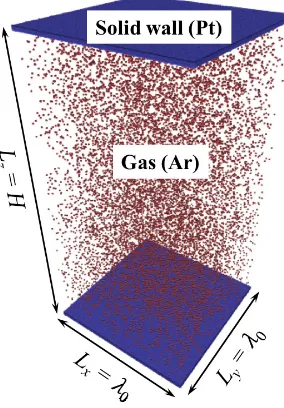
FIG. 2: MD simulation: sample configuration of argon (Ar) gas confined in a microchannel at
standard temperature and pressure.
case. The MD results reported below use these numbers of bins.
III. RESULTS AND DISCUSSION
A. Mean free path of confined gases
We consider a gas in equilibrium at standard temperature and pressure confined in a
microchan-nel and evaluate the MFPs using both DSMC and the MD techniques. In the DSMC simulations,
the computational domain is one-dimensional (zdirection). In the MD simulations, the two solid
walls are parallel to thexyplane and periodic boundary conditions are imposed along thexandy
directions, as shown in Fig. 2. The distance between the two parallel walls in thezdirection isH,
and the lengths in both xand ydirections are set to λ0, which is the nominal MFP. We simulate
cases with different z-direction distances between the two parallel walls, varying from 20λ0 to
λ0/2, whereλ0is the nominal MFP given by Eq. (3). These correspond to Kn ranging from 0.05
to 2.
As the collisions between gas molecules and wall atoms are momentum-changing events, we
have taken these into account when recording the free paths. However, below we also investigate
(a) Kn = 0.05, 0.1, 0.2 (b) Kn = 0.5, 1, 2
FIG. 3: Probability density distribution of the individual free paths of gas molecules in the
middle of channels provided by MD and DSMC simulations for different Knudsen numbers: (a)
Kn = 0.05, 0.1, 0.2 and (b) Kn = 0.5, 1, 2.
The influence of a solid wall on the MFP can be first investigated by examining the probability
distribution of the individual free paths across the channel. In elementary kinetic theory, the free
path distribution of gas molecules is supposed to be exponential in a homogeneous system (i.e.
when the gas is not bounded by solid surfaces), which we verify is the case in both our MD
and DSMC simulations. However, the free path of gas molecules can be terminated at the wall
in confined geometries (i.e. an inhomogeneous case) if gas-wall collisions are counted, which
produces a power-law distribution of the free paths17. Therefore, to assess the effect of solid walls,
we measure the free path distributions of gas molecules in the middle of channels with different
heights. Figure 3(a) shows that the free path distributions are still essentially exponential at small
Kn (i.e. in the upper slip and early transition regimes). However, as shown in Fig. 3(b), when
Kn&0.5, spikes are observed in the distributions of the free paths; these spikes are caused by the
presence of the solid walls and move to the smaller free paths as Kn increases. The simulation
results of the DSMC and MD are in good agreement.
As can be seen in Fig. 4, the measured MFP varies near the wall, and at the wall is half the
nominal value it has in the bulk. It is worth stressing that the small spatial gap between the surface
in a measurement bin to the central point of that bin; this becomes more noticeable at larger Kn.
The spatial extent of the near-wall zone becomes greater with increasing Kn. At small Kn, the
MD results agree well with the DSMC results and Abramov’s theoretical prediction1, i.e. Eq. (6),
while the expression of Guoet al.20, i.e. Eq. (5), somewhat underpredicts the MFP near the walls.
Note that Toet al.39 obtained a MFP of zero near the wall in their MD simulations for Kn = 0.18
and 0.37, but they only considered molecules outgoing from the walls.
As mentioned earlier, authors from a previous study7 have argued that the MFP should be
defined as the average distance between successive collisions of gas molecules only, and that
collisions between gas molecules and wall atoms or gas molecules adsorbed on a wall surface
should not be taken into account when evaluating individual free paths. With such a definition,
a constant and isotropic MFP would be expected. In order to assess this prediction, we have run
MD and DSMC simulations in a microchannel (H =20λ0) and disregarded gas-wall collisions in
the evaluation of the MFP. More specifically, while interactions between gas molecules and wall
atoms are still part of the dynamics, the individual free paths are not terminated at the walls. Our
simulations show that a constant MFP is predicted by both DSMC and MD simulations when the
walls are perfectly specular (i.e. α =0), and Fig. 5 shows that a constant MFP is also obtained
when fully diffusive (DSMC) and real (MD) walls are used.
We therefore conclude that a space-dependent MFP in confined geometries (i.e. an
inhomoge-neous case) is simply a consequence of taking into account the gas-wall collisions. This result is
not in disagreement with the classical expression in kinetic theory that relies on the assumption
of spatially homogeneous conditions. Collisions between the gas and bounding surfaces can be
incorporated in the concept of the MFP and, as discussed in the literature1,2,5,20,39, the resulting
spatial variation of the MFP may help in understanding the transport of gases in Knudsen layers
near surfaces.
B. Local viscosity of the gas in near-wall regions
If the MFP is constant in micro/nanochannels, i.e. the collision rate is on average constant
everywhere, this indicates that the viscosity of the fluid behaves homogeneously too, and the
system under a constant shear stress should give a linear velocity profile. We know that this is
not true for gases in thermodynamic non-equilibrium, and we believe the hypothesis that there
FIG. 4: Spatial variation of the normalised MFP in microchannels using DSMC (open squares)
and MD (open circles). The theoretical predictions of Guoet al.20 (blue solid line) and Abramov2
(green solid line) are also included for comparison. Data are plotted for only half the channel (i.e.
above one of the surfaces).
FIG. 5: Spatial variation of the normalised MFP of the gas in a microchannel (H=20λ0). Red
and green solid lines refer to the DSMC simulation results that count and do not count the
gas-wall collisions, respectively; Open squares (black) and circles (blue) refer to the MD
simulation results that count and do not count the gas-wall collisions, respectively. Data are
[image:13.612.195.413.399.615.2]viscosity, such as in Eqs. (1) and (2), is appealing because it allows us to use a modified version
of the ubiquitous hydrodynamic Navier-Stokes equations for solving rarefied gas flows, without
the large computational expense of DSMC or MD. However, whether this “effective viscosity” is
actually effective or is physical, are still unclear. It is also worth stressing that it is not unreasonable
that the transport properties of dense fluids in micro/nanochannels differ from those determined
in bulk, especially when their are strong inhomogeneities near the confining walls, such as water
flows through nanotubes or nanopores9,15,18,33,45. The channel heights we are considering in this
work are however very large in comparison to the few nanometer dimensions, where such
non-continuum transport behaviour are seen to deviate from their bulk description.
In this section we measure viscosity using two independent approaches for three of the lower
Knudsen number cases. In the first approach we run Couette simulations and calculate viscosity
using the linear stress-strain relationship:
µ(z) =−hPxz(z)i
hγ˙(z)i , (10)
wherePxz and ˙γ are the shear stress parallel to the solid wall and the rate of strain, respectively,
and the angle brackets denote a time-averaged value from the MD simulations. Note that since
the gas is rarefied, no layering occurs at the walls and, therefore, the application of this method
is anticipated not to suffer any singularity issues45. In Eq. (10), the stress tensor is calculated by
using the Irving-Kirkwood approach21, i.e.
P = 1
V "
∑
i
mi(vi−u)2+
1
2
∑
i,jri jFi j #, (11)
in whichV is the bin volume,vi is the velocity of theith gas molecule, r is the relative position
between two molecules,uis the local average velocity of the gas flow, andF is the force between
two molecules. The first term on the right-hand side of Eq. (11) is the kinetic component, and the
second one is the virial component. The kinetic term in the Irving-Kirkwood expression is related
to the ideal-gas law, whereas the molecular-molecular virial terms are corrections to the ideal-gas
law needed to account for volumes and the force fields between interacting molecules6.
In the Couette flow problem the gas is sheared by both top and bottom walls, which move with a
constant velocityu0=0.2σAr/τin opposite directions along thexaxis. This velocity is sufficiently
small for thermal effects to be neglected, i.e. the gas flow is isothermal and incompressible. The
computational domain is the same as shown in Fig. 2. That is, the distance between the two parallel
20λ0, 10λ0, 5λ0, which corresponds to Kn = 0.05, 0.1, 0.2, and, in all these cases, the channel in
thezdirection is divided into 21 number of bins. The distributions of the strain rate and shear stress
across the channel are calculated from the local gradient of the velocity profile and from Eq. (11),
respectively. The shear stress and the rate of strain have been averaged over 3×10⁶time steps after
the system reached a steady state. A velocity-rescaling thermostat was applied to molecules in the
y-direction only, in order to prevent the flow from being perturbed. Figure 6 then shows the local
viscosity of the gas across the channel deduced from the linear-response relationship, i.e. Eq. (10).
It is apparent that the gas viscosity varies near a solid surface, decreasing with increasing Kn. We
observe that the gas viscosity at the wall reduces almost to half the value it has in the bulk (i.e.
49% for Kn = 0.05, 48% for Kn = 0.1, and 44% for Kn = 0.2).
In our second approach we use the Green-Kubo (G-K) equation:
µ = V
kBT
Z ∞
0
hPxz(0)Pxz(t)idt, (12)
whereV is the volume, and the time integration is the ensemble average of the auto-correlation of
the stress tensor Pxz. The same Kn cases are used as our first method, but now have no moving
walls; i.e. there is no flow, and we also divide the system in 7 bins to determine the variation in
viscosity. Each case is made larger in the x andy coordinates in order to make the bins contain
a large number of molecules for the auto correlation function (ACF), and have a shape which are
closer to being cubic. Therefore, for Kn = 0.05, 0.1, 0.2 we changed Lx,Ly to 1.5λ0, 2λ0, 3λ0.
Each simulation was run for 40 million time steps, and the ACF is averaged over successive 200k
time steps. No thermostat was applied during the measurement of viscosity.
Note, in principle, Eq. (12) only applies to homogeneous systems in the bulk limit but it has
been widely used for evaluating the transport coefficients of confined fluids as well11,19,38. Here we
use the qualitative behaviour of the viscosity from the G-K approach using the largest possible bins
we could, as we were not able to produce the same level of resolution as the other two techniques,
without running into issues of noise and large computational costs.
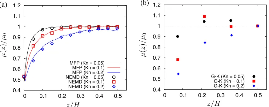
We plot in Fig. 6 three independent scaled viscosity calculations: a) the results from our MFP
measurements, i.e. Eq. (1), b) the results from the Couette flow, i.e. Eq. (10) and c) the results from
Green-Kubo, i.e. Eq. (12). Generally, good agreement is achieved across all three methods.
The viscosity seems to drop by half near the solid wall, and recovers the bulk value for Kn =
0.05 and Kn = 0.1. At Kn = 0.2, viscosity measurements still seem to match up well, but
0.4 0.5 0.6 0.7 0.8 0.9 1 1.1 1.2
0 0.1 0.2 0.3 0.4 0.5 G-K (Kn = 0.05)
G-K (Kn = 0.1) G-K (Kn = 0.2)
(a) (b) 0.4 0.5 0.6 0.7 0.8 0.9 1 1.1 1.2
0 0.1 0.2 0.3 0.4 0.5 MFP (Kn = 0.05)
[image:16.612.89.526.74.249.2]MFP (Kn = 0.1) MFP (Kn = 0.2) NEMD (Kn = 0.05) NEMD (Kn = 0.1) NEMD (Kn = 0.2)
FIG. 6: Local viscosity measurements of gases predicted using (a) the MFP-based scaling law,
Eq. (2) and the non-equilibrium MD (NEMD) simulations of Couette flow, Eq. (10), and (b) the
Green-Kubo (G-K), Eq. (12), for Kn = 0.05, 0.1, and 0.2. Data are plotted for only half the
channel (i.e. above one of the surfaces), andµ0is taken to be the bulk viscosity.
Knudsen layers. It is unclear at which stage the definition of viscosity stops being local in rarefied
gases. Our work seems to show that it is still relatively accurate to use spatial variations of viscosity
up to the early transition Knudsen regime, at least in these simple shear flows.
IV. CONCLUSIONS
The molecular mean free path (MFP) in a confined gas has been numerically evaluated using
both the direct simulation Monte Carlo (DSMC) and molecular dynamics (MD) simulations. The
MFP has been found to drop smoothly to half of its bulk value near the walls, as long as the
collisions between the gas and the wall are accounted for. We demonstrate that the wall-distance
dependent MFP is not a numerical artefact but rather a consequence of taking into account the
collisions between gas and wall molecules in the calculation of the MFP locally.
In this respect, two main conclusions are made. First, these results are not in disagreement
with elementary kinetic theory expressions for the MFP, since these expressions only refer to a
spatially homogeneous gas. Second, the answer to the question of whether or not the definition
of the MFP should take into account collisions with the solid surfaces depends on the purpose for
which the MFP is intended. If it is used to scale transport properties near walls2,5,17,20,39, then a
spatially-varying viscosity derived from the MFP, which agrees well with independent measurements of
viscosity using Newton’s equation of viscosity from a non-equilibrium Couette flow as well as the
Green-Kubo formulation.
The numerical results obtained in the present study have also permitted to assess the theoretical
scaling laws for the MFP proposed in the literature so far2,20. It turned out that Abramov’s scaling
law provides the best match with both MD and DSMC results.
A number of future research directions can be envisioned. These include a more detailed
analy-sis of the capability of the MFP-based viscosity to describe gas flows in the early transition regime
(including in more complex geometries), as well as the development of a consistent slip boundary
conditions to be used within this mathematical framework.
V. ACKNOWLEDGEMENTS
The authors would like to acknowledge the work of Graeme Bird. His influence on the rarefied
gas dynamics community has been profound, and through direct and indirect routes inspired the
work in this paper, and many others. Finally, the authors would like to dedicate this article to Jason
Reese, our co-author, mentor and friend, who passed away in March 2019.
The work is financially supported by the UK’s Engineering and Physical Sciences Research
Council (EPSRC) via grant nos. EP/N016602/1 and EP/R007438/1. JMR acknowledges the
sup-port of the Royal Academy of Engineering under the Chair in Emerging Technologies scheme.
JFX thanks the National Natural Science Foundation of China (grant no. 51506110) for their
support. OH acknowledges support from the EPSRC Early Career Research Software Engineer
Fellowship Scheme (EP/N019180/2). The authors thank Dr Srinivasa Ramisetti for useful
discus-sions.
Appendix A: MD Calibration procedure
In order to directly evaluate the MFP in MD simulations with a continuous interaction potential,
a procedure for judging the collision event between two molecules is required, and a collision
diameter should be chosen. For argon molecules, Dongariet al.17 and Perumanath Dharmapalan
et al.31 suggestedσcol =σAr, while Barisik and Beskok7 usedσcol =1.06σAr by combining the
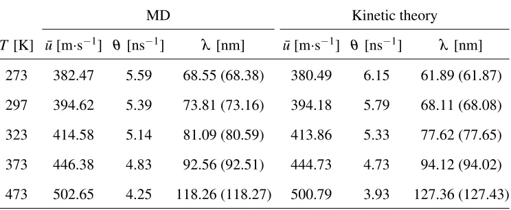
TABLE II: Comparison of the MFP for a spatially homogeneous gas provided by MD
simulations withσcol =σAr and kinetic theory. The values of MFP in brackets are from the ratio
of the mean velocity ¯uto collision frequencyθ, i.e.λ =u/¯ θ.
MD Kinetic theory
T [K] ¯u[m·s−1] θ[ns−1] λ [nm] u¯[m·s−1] θ [ns−1] λ [nm]
273 382.47 5.59 68.55 (68.38) 380.49 6.15 61.89 (61.87)
297 394.62 5.39 73.81 (73.16) 394.18 5.79 68.11 (68.08)
323 414.58 5.14 81.09 (80.59) 413.86 5.33 77.62 (77.65)
373 446.38 4.83 92.56 (92.51) 444.73 4.73 94.12 (94.02)
473 502.65 4.25 118.26 (118.27) 500.79 3.93 127.36 (127.43)
Note that, in fact,λhandλvdiffer by a small multiplicative constant:λh/λv=16/5π=1.0228. To
et al.39adoptedσcol=1.014σAr as a best fit of the predictions of kinetic theory to their calculations
of MFP using MD.
To demonstrate the sensitivity of the MFP measurements to the collision diameter, we consider
the MFP of argon molecules contained in a cubic domain, with periodic boundary conditions
in all directions with the length of each side of the domain set to about one MFP, as given by
Eq. (4). We set σcol =σAr and we see in Table II that the subsequent values of MFP from our
MD simulations are greater than kinetic theory predictions at low gas temperatures, but smaller at
higher gas temperatures. This is not unexpected because molecules have larger kinetic energies at
high temperatures and this reduces the collision diameter. The averaged value of the free paths can
also be obtained by the ratio of the mean velocity of the gas molecules to the collision frequency
between gas molecules, i.e. λ =u/¯ θ, where the mean velocity is ¯u=p8kBT/πm, andθ is the
collision frequency given by MD. A comparison of the averaged free paths based on the collision
frequency and the MFP determined directly from our MD simulations is also made in Table II, and
there is a generally good agreement between the two approaches.
In order to recover the kinetic theory prediction of the MFP, i.e. Eq. (4), a
temperature-dependent collision diameter is proposed to characterise the collision events between gas molecules.
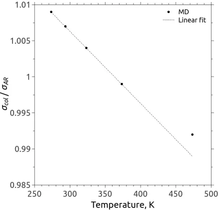
(a) MFP versus the collision diameter at 273 K. (b) Collision diameter versus temperature.
FIG. 7: Calibration study of the collision diameterσcol for argon in a spatially-homogeneous
MD system, where (a) shows the calibration of the collision diameter for a fixed temperature of
273 K that provides the same mean free path as kinetic theory, and (b) shows the final calibrated
collision diameters of various temperatures.
at a low gas temperature (i.e. 273 K) for varying prescribedσcol (filled circles). The MD-measured
MFP decreases with the increase of the collision diameter, and the intersection with the prediction
of kinetic theory, Eq. (4) (red solid line), is when σcol '1.009σAr. Likewise, the approximate
collision diameter can be determined over a range of temperatures, and the results are shown
by solid black symbols in Fig. 7(b). The collision diameter decreases as the gas temperature
increases, and in the range of explored temperatures a linear relationship can be estimated, i.e.
σcol(T)/σAr =1.0363−0.0001T with T up to 373 K. As the gas temperature increases (∼473
K), the decrease of collision diameter becomes less pronounced and a deviation from the linear fit
is observed. Nevertheless, the proposed temperature-dependent collision diameter can guarantee
good agreement of the MFP between MD calculations and predictions of kinetic theory for the
explored gas temperatures.
Note that, in principle, a temperature-dependent collision diameter can be defined based on the
Chapman-Enskog expression of the viscosity for a gas composed of hard spheres13:
d2h= 5
16 1
µ
r kBT
whereµ(T)is the viscosity of LJ fluids13,30. However, the collision diameters predicted based on
Eq. (A1) differ significantly from the ones provided by MD simulations. Therefore, the calibration
procedure described above turns out to be necessary in order to get accurate simulation results.
REFERENCES
1Abramov, R. V., “Diffusive boltzmann equation, its fluid dynamics, couette flow and knudsen
layers,” Physica A484, 532–557 (2017).
2Abramov, R. V., “Gas near a wall: Shortened mean free path, reduced viscosity, and the
man-ifestation of the knudsen layer in the navier–stokes solution of a shear flow,” J. Nonlinear Sci.
28, 833–845 (2018).
3Allen, M. P. and Tildesley, D. J.,Computer Simulation of Liquids(Clarendon, Oxford, 1987).
4Aristov, V., Direct Methods for Solving the Boltzmann Equation and Study of Nonequilibrium
Flows(Springer, 2001).
5Arlemark, E. J., Dadzie, S. K., and Reese, J. M., “An extension to the Navier-Stokes equations
to incorporate gas molecular collisions with boundaries,” J. Heat Transf.132, 041006 (2010).
6Barisik, M. and Beskok, A., “Equilibrium molecular dynamics studies on nanoscale-confined
fluids,” Microfluidics Nanofluid.11, 269–282 (2011).
7Barisik, M. and Beskok, A., “Molecular free paths in nanoscale gas flows,” Microfluidics
Nanofluid.18, 1365–1371 (2015).
8Bird, G. A.,Molecular Gas Dynamics and the Direct Simulation of Gas Flows(Oxford
Univer-sity Press, Oxford, 1994).
9Borg, M. K., Lockerby, D. A., Ritos, K., and Reese, J. M., “Multiscale simulation of water flow
through laboratory-scale nanotube membranes,” Journal of Membrane Science567, 115 – 126
(2018).
10Cao, B. Y., Chen, M., and Guo, Z. Y., “Temperature dependence of the tangential momentum
accommodation coefficient for gases,” Appl. Phys. Lett.86, 091905 (2005).
11Casanova, S., Borg, M. K., Chew, Y. M. J., and Mattia, D., “Surface-controlled water flow in
nanotube membranes,” ACS Applied Materials & Interfaces11, 1689–1698 (2019).
12Cercignani, C.,Slow Rarefied Flows: Theory and Application to Micro-Electro-Mechanical
Sys-tems(Birkhäuser Verlag, Basel - Boston - Berlin).
the kinetic theory of viscosity, thermal conduction and diffusion in gases(Cambridge University
Press, Cambridge, 1970).
14Darabi, H., Ettehad, A., Javadpour, F., and Sepehrnoori, K., “Gas flow in ultra-tight shale strata,”
J. Fluid Mech.710, 641658 (2012).
15Davis, H., “Kinetic theory of flow in strongly inhomogeneous fluids,” Chem. Eng. Comm. 58,
413–430 (1987).
16Dimarco, G. and Pareschi, L., “Numerical methods for kinetic equations,” Acta Numer.23, 369–
520 (2014).
17Dongari, N., Zhang, Y., and Reese, J. M., “Molecular free path distribution in rarefied gases,” J.
Phys. D Appl. Phys.44, 125502 (2011).
18Evans, D. J. and Morriss, G.,Statistical mechanics of nonequilibrium liquids(Cambridge
Uni-versity Press, 2008).
19Giannakopoulos, A., Sofos, F., Karakasidis, T., and Liakopoulos, A., “Unified description of
size effects of transport properties of liquids flowing in nanochannels,” Int. J. Heat Mass Transf.
55, 5087–5092 (2012).
20Guo, Z. L., Shi, B. C., and Zheng, C. G., “An extended Navier-Stokes formulation for gas flows
in the knudsen layer near a wall,” Europhys. Lett.80, 24001 (2007).
21Irving, J. and Kirkwood, J., “The statistical mechanical theory of transport processes. iv. the
equations of hydrodynamics,” J. Chem. Phys.18, 817–829 (1950).
22Jiang, S. and Luo, L.-S., “Analysis and accurate numerical solutions of the integral equation
derived from the linearized bgkw equation for the steady couette flow,” J. Comput. Phys. 316,
416–434 (2016).
23Kennard, E. H., Kinetic Theory of Gases (McGraw-Hill Book Company, Inc., New York and
London, 1938).
24Li, W., Luo, L.-S., and Shen, J., “Accurate solution and approximations of the linearized bgk
equation for steady couette flow,” Comput. Fluids111, 18–32 (2015).
25Lilley, C. R. and Sader, J. E., “Velocity gradient singularity and structure of the velocity profile
in the knudsen layer according to the boltzmann equation,” Phys. Rev. E76, 026315 (2007).
26Lockerby, D. A., Reese, J. M., and Gallis, M. A., “Capturing the Knudsen layer in
continuum-fluid models of nonequilibrium gas flows,” AIAA Journal43, 1391–1393 (2005).
27Lorenzani, S., Gibelli, L., Frezzotti, A., Frangi, A., and Cercignani, C., “Kinetic approach to
28Morris, D. L., Hannon, L., and Garcia, A. L., “Slip length in a dilute gas,” Phys. Rev. A 46,
5279–5281 (1992).
29Muntz, E. P., “Rarefied gas dynamics,” Annu. Rev. Fluid Mech.21, 387–422 (1989).
30Neufeld, P. D., Janzen, A., and Aziz, R., “Empirical equations to calculate 16 of the transport
collision integrals ω(l,s)∗ for the Lennard-Jones (12-6) potential,” J. Chem. Phys. 57, 1100–
1102 (1972).
31P.D., S. H., Prabha, S. K., and Sathian, S. P., “The effect of characteristic length on mean free
path for confined gases,” Physica A437, 68–74 (2015).
32Plimpton, S., “Fast parallel algorithms for short-range molecular dynamics,” J. Compt. Phys.
117, 1–19 (1995).
33Pozhar, L. A., “Structure and dynamics of nanofluids: Theory and simulations to calculate
vis-cosity,” Phys. Rev. E61, 1432 (2000).
34Rapaport, D. C.,The Art of Molecular Dynamics Simulation(Cambridge University Press,
Cam-bridge, 1995).
35Reese, J. M., Gallis, M. A., and Lockerby, D. A., “New directions in fluid dynamics:
non-equilibrium aerodynamic and microsystem flows,” Philos. T. Roy. Soc. A 361, 2967–2988
(2003).
36Stops, D. W., “The mean free path of gas molecules in the transition regime,” J. Phys. D Appl.
Phys.3, 685–696 (1970).
37Struchtrup, H.,Macroscopic Transport Equations for Rarefied Gas Flows(Springer, 2005).
38Thomas, J. A. and McGaughey, A. J. H., “Reassessing fast water transport through carbon
nan-otubes,” Nano Letters8, 2788–2793 (2008).
39To, Q. D., Léonard, C., and Lauriat, G., “Free-path distribution and Knudsen-layer modeling
for gaseous flows in the transition regime,” Phys. Rev. E91, 023015 (2015).
40Wagner, W., “A convergence proof for bird’s direct simulation monte carlo method for the
boltz-mann equation,” J. Stat. Phys.66, 1011–1044 (1992).
41Wu, L., Ho, M. T., Germanou, L., Gu, X.-J., Liu, C., Xu, K., and Zhang, Y., “On the apparent
permeability of porous media in rarefied gas flows,” J. Fluid Mech.822, 398–417 (2017).
42Xie, J.-F. and Cao, B.-Y., “Fast nanofluidics by travelling surface waves,” Microfluidics
Nanofluid.21, 111 (2017).
43Xie, J.-F., Sazhin, S. S., and Cao, B.-Y., “Molecular dynamics study of the processes in the
44Zhang, J., Fan, J., and Fei, F., “Effects of convection and solid wall on the diffusion in microscale
convection flows,” Phys. Fluids22, 122005 (2010).
45Zhang, J., Todd, B., and Travis, K. P., “Viscosity of confined inhomogeneous nonequilibrium