Time dependent stick breaking processes

University of Warwick institutional repository: http://go.warwick.ac.uk/wrap

This paper is made available online in accordance with

publisher policies. Please scroll down to view the document

itself. Please refer to the repository record for this item and our

policy information available from the repository home page for

further information.

To see the final version of this paper please visit the publisher’s website

.

Access to the published version may require a subscription.

Author(s): JE Griffin and MFJ Steel

Article Title: Time-Dependent Stick-Breaking Processes

Year of publication: 2009

Link to published article:

http://www2.warwick.ac.uk/fac/sci/statistics/crism/research/2009/paper

09-05

Time-Dependent Stick-Breaking Processes

J.E. Griffin

Institute of Mathematics, Statistics and Actuarial Science,

University of Kent, U.K.

M. F. J. Steel

Department of Statistics, University of Warwick, U.K.

Abstract

This paper considers the problem of defining a time-dependent nonparametric prior. A

recur-sive construction allows the definition of priors whose marginals have a general stick-breaking form.

The processes with Poisson-Dirichlet and Dirichlet process marginals have interesting

interpreta-tions that are further investigated. We develop a general conditional Markov Chain Monte Carlo

(MCMC) method for inference in the wide subclass of these models where the parameters of the

stick-breaking process form increasing sequences. We derive a P´olya urn scheme type

representa-tion of the Dirichlet process construcrepresenta-tion, which allows us to develop a marginal MCMC method

for this case. The results section shows the relative performance of the two MCMC schemes for the

Dirichlet process case and contains three real data examples.

∗_{Corresponding author: Jim Griffin, Institute of Mathematics, Statistics and Actuarial Science, University of Kent,} Can-terbury, CT2 7NF, U.K. Tel.: +44-1227-823627; Fax: +44-1227-827932; Email: [email protected]. The authors

would like to acknowledge helpful comments from seminar audiences at the Universities of Newcastle, Nottingham, Bath,

Keywords: Bayesian Nonparametrics, Dirichlet Process, Poisson-Dirichlet Process, Time-Dependent

Nonparametrics.

1 Introduction

Nonparametric estimation is an increasingly important element in the modern statistician’s toolbox.

The availability of efficient methods for the estimation of unknown distribution has lead to the

de-velopment of regression methods that allow many unknown distributions to be estimated jointly.

Recently, there has been interest in extending standard Bayesian nonparametric methods,

particu-larly the Mixture of Dirichlet Processes (Antoniak 1974) to regression and time series contexts (e.g.

De Iorioet al2004, M¨ulleret al2004, Griffin and Steel 2006 and Dunsonet al2007). The

devel-opment of methodology is generally difficult because we must define a measure-valued stochastic

process. In this paper we will work exclusively on the time series problem, which often allows

simpler constructions.

Time-dependent nonparametric priors have been used in a wide-range of applications. Two

ex-treme examples would be: the observation of a single time series over a long time period such as a

stock index considered by Griffin and Steel (2006) and Caronet al(2007). On the other hand we

can consider many observations at each time pointe.g.travel claims considered by Rodriguez and

ter Horst (2008). We assume observations are independently drawn conditional on the unknown

distributions. Therefore longitudinal data cannot be directly modelled but can be modelled

hierar-chically (Dunson 2006) using these models. If we have a long time series, we need strong prior

assumptions for effective inference. In the second case, we have more information at each time

point (e.g.we could make inference about the distribution at each time point independently) but our

aim is to estimate and exploit the relationship between distributions at each time point.

then a Bayesian nonparametric analysis could assume that their conditional can be expressed as

f_ti(y_i) =

Z

k(y_i|ϕ_i)dG_ti(ϕ_i) (1)

Gti =

∞

X

j=1

pj(ti)δθj(ti)

for some density functionk(·), wherep1, p2, p3, . . . sum to one and are independent ofθ1, θ2, θ3, . . .

whileδθ is the Dirac delta function which places measure 1 on the pointθ. This implies that (1)

defines a mixture of parametric distributions with mixing distributionG_ti. The model reduces to

a species sampling mixture model if all the observations are taken at a single time. The class of

species sampling mixture models includes Dirichlet Process Mixtures (Lo 1984), Stick-Breaking

Mixtures (Ishwaran and James 2001, 2003), and Normalized Random Measure mixtures (Jameset

al2005). If we assume thatp_j(t) =p_j for allt, the model reduces to an infinite mixture of

time-series model in the framework of Dependent Dirichlet Processes. Rodriguez and ter Horst (2008)

develop methods in this direction. Alternatively, several constructions make the assumption that

θj(t)does not depend on time and soθj(t) =θj for allt. Examples in continuous time include the

Ornstein-Uhlenbeck Dirichlet Process (Griffin 2007) and the “arrivals” construction of theπ-DDP

(Griffin and Steel 2006) and in discrete time include the Time Series Dependent Dirichlet Process

(Nieto-Barajas et al, 2008). Zhuet al (2005) model the distribution function of the observables

directly by defining a Time-Sensitive Dirichlet Process which generalizes the P´olya urn scheme of

the Dirichlet process to

G_t|y∝I(t_i < t) exp{−(t−t_i)}δ_yi+M H

wheretiis the time at whichyiis observed andM andHare the mass parameter and the centring

distribution of the Dirichlet process. The influence of an observation at timetidecreases ast−ti

becomes large. However, the process is not consistent under marginalisation of the sample. A

related approach is described by Caronet al(2007). In discrete time, Dunson (2006) proposes the

evolution

Gt=πGt−1+ (1−π)²t

whereπis a parameter and²tis a realisation from a Dirichlet process. This defines an AR-process

similarities to the “arrivals”π-DDP in discrete time, where the model is generalized to

Gt=πt−1Gt−1+ (1−πt−1)²t−1

where²t is a discrete distribution with a Poisson-distributed number of atoms andπtis a random

variable correlated with²t. Griffin and Steel (2006) show how to ensure that the marginal law ofGt

follows a Dirichlet process for allt.

This paper extends the literature on time-dependent nonparametric priors in a number of ways:

1) we describe and study in detail a construction of a measure-valued stochastic process with any

given stick-breaking process as the marginal process, 2) we define a Markov chain Monte Carlo

(MCMC) scheme for inference with a wide subclass of these process (including the

Poisson-Dirichlet process), and 3) we derive P´olya urn-type schemes for the important special case of a

Dirichlet process marginal.

The paper is organised in the following way: Section 2 describes the link between stick-breaking

processes and time-varying nonparametric models and presents a method for constructing stationary

processes with a given marginal stick-breaking process. Section 3 discusses two important special

cases: Dirichlet process and Poisson-Dirichlet marginals. Section 4 briefly describes the proposed

computational methods. In Section 5 we analyse some simulated data and explore three econometric

examples using the two leading processes. Proofs of all Theorems are grouped in Appendix A,

whereas Appendix B presents details of the MCMC algorithms.

2 Time-dependent nonparametric priors and stick-breaking

In this paper, we will work exclusively with the model in (1) where θj(t) = θj for all t. An

important characteristic of (1) is thatGtis discrete at all times, which can make seemingly natural

generalisations of standard time series model have unusual properties. For example, we can define

a random walky1, y2, y3, . . . with normal increments equivalently as:

where N(µ, σ2)denotes the normal distribution with meanµand varianceσ2, or

yi =yi−1+²iwhere²1, ²2, . . . are i.i.d. N(0, σ2). (3)

This equivalence does not extend naturally to infinite discrete distributions. Suppose that we wanted

to generalize (2) we might define

Gt|Gt−1∼DP(M, Gt−1) (4)

where DP(α, G)represents a Dirichlet process with mass parameterαand centring distributionG.

Under this model, the variance of the mass assigned to some setBwill be

Var[Gt+j(B)|Gt−1] =αjGt−1(B) [1−Gt−1(B)],

whereα_j is an increasing sequence depending onM and tending to 1 asj→ ∞. The variability is

increasing withj, which we would want, but, sinceGt+j is a discrete distributions, the maximum

variability arises when our distribution is a single point mass at some value drawn fromGt−1. A

natural generalisation of (3) is

Gt= (1−Vt)Gt−1+Vt²t

where ²t is a random probability distribution (with infinite or finite numbers of atoms) which is

independent ofG_t−1. The latter construction does not suffer from this degeneracy problem. The degeneracy of the process defined by (4) is similar to the phenomenon of particle depletion in

par-ticle filters that is caused by the approximation of a continuous distribution by a finite, discrete

distribution (seee.g.Doucetet al2001). These problems are addressed through a so-called

rejuve-nation step where randomness is introduced into the distribution of particles. Adding an innovation

at each time step will have a similar effect in these models.

We now focus on the choice of Vt and²t. If²tis a discrete distribution thenGt will also be

discrete at all times. If we further restrict²tto be a single atom at a pointθtdrawn at random from

Hthen each marginal distribution naturally has a so-called “stick-breaking” structure since we can

write

Gt= t X

i=−∞

δθiVi

t Y

j=i+1

where stick-breaking is applied backwards in time (the atom introduced at timethas the largest

expected weight). More formally, the stick-breaking construction of random probability measures

(Pitman 1996, Ishwaran and James 2001) is defined as follows

Definition 1 Suppose thata = (a1, a2, . . .) andb = (b1, b2, . . .)are sequences of positive real

numbers. A random probability measureGfollows a stick-breaking process if

G=d ∞

X

i=1

piδθi

pi =Vi Y

j<i

(1−Vj)

whereθ1, θ2, θ3,· · ·i.i.d.∼ HandV1, V2, V3, . . . is a sequence of independent random variables for

whichVi ∼Be(ai, bi)for alli. This process will be written asG∼Π(a,b, H).

Ishwaran and James (2001) shows that the process is well-defined (i.e.P∞_i=1pi = 1almost surely)

if

∞

X

i=1

log(1 +ai/bi) =∞.

A number of standard processes fall within this class. The two most widely used are the Dirichlet

process whereaj = 1andbj =M and the Poisson-Dirichlet (or Pitman-Yor) processaj = 1−a,

b_j = M +aj (with 0 ≤ a < 1, M > −a). The Dirichlet process has been almost ubiqitous

in applications of Bayesian nonparametric model. The Poisson-Dirichlet process was discussed in

some detail in Pitman and Yor (1997) and James (2008) and has been used bye.g.Teh (2006).

Griffin and Steel (2006) shows that if we choose Vj ∼ Be(1, M) then the process in (5) is

stationary in the sense thatGt will have the same stick-breaking prior as Gs for all sandt and

“mean-reverting” in the sense that E[Gt] → H ast → ∞. They further subordinate the process

in (5) to some additive process,Xt, which allows modelling of the autocorrelation structure whilst

maintaining a marginal Dirichlet process. If the additive process is a stationary Poisson process

with intensityλthen the autocorrelation has an exponential form

Corr(Gt, Gt+k) = exp ½

− λk

M+ 1

¾

This naturally leads to two questions: 1) how can we construct processes whose margins follows a

specific stick-breaking process? And 2) how can we control the autocorrelation of the process of

distributions{Gt}∞t=−∞?

To develop answers to these questions we will initially work with an extension of the discrete

time process in (5) and then extend to continuous time by subordination. The model in (5) naturally

includes the marginal two-parameter Beta processes (Ishwaran and Zarepour 2000) which arise by

assuming thatVi ∼ Be(a, M). However, if the distributions of theVi’s depends on the ordering,

we need to account for that since the ordering of the atoms evolves over time. Thus, such marginal

stick-breaking processes can only arise from the generalized model

Gt= t X

i=−∞

δθiVi,t−i+1

t Y

j=i+1

(1−Vj,t−j+1), (6)

whereVj,1, Vj,2, . . . denotes the value of the break introduced at timejas it evolves over time and

Vj,t represents its value at timej+t. The stochastic processes {Vi,t}∞t=1 and{Vj,t}∞t=1 must be

independent fori 6=j if the processGtis to have a stick-breaking form. If we wantGtto follow

a stick-breaking process with parametersaandbthen the marginal distribution ofVi,twould have

to be distributed Be(at, bt)for alliandtand clearly we need time dependence of the breaks. The

following theorem allows us to define a reversible stochastic process Vi,t which has the correct

distributions at all time points to define a stationary process whose marginal process has a given

stick-breaking form. In the following theorem we define that if X is distributed Be(a,0) then

X = 1with probability 1 and ifXis distributed Be(0, b)thenX = 0with probability 1. We will

use the notation Ga(a)to denote a Gamma distribution with shapeaand unitary scale.

Theorem 1 Suppose that Vj,t ∼ Be(at, bt) andVj,t+1 ∼ Be(at+1, bt+1) then the following

rela-tionships maintain the marginal distributions:

Case (i) Ifa_t+1≥a_tandb_t+1 ≥b_t

V_j,t+1=w_j,t+1V_j,t+ (1−w_j,t+1)²_j,t+1

Case (ii) Ifat+1≤atandbt+1 ≤bt

Vj,t+1 =

w_j,t+1V_j,t

wj,t+1Vj,t+ (1−wj,t+1)(1−Vj,t)

wherewj,t= _xj,tx₊j,t_zj,t andxj,t ∼Be(at+1, at−at+1)andzj,t∼Be(bt+1, bt−bt+1).

Case (iii) Ifat+1≤atandbt+1 ≥bt

Vj,t+1= _x xj,tVj,t

j,tVj,t+ 1−xj,t+zj,t wherexj,t ∼Be(at+1, at−at+1)andzj,t ∼Ga(bt+1−bt).

Case (iv) Ifat+1≥atandbt+1 ≤bt

Vj,t+1 = _x zj,tVj,t

j,t(1−Vj,t) +zj,t+Vj,t wherexj,t ∼Be(at+1, at−at+1)andzj,t ∼Ga(bt+1−bt).

The application of this theorem allows us to construct stochastic processes with the correct

margins for any stick-breaking process. We will concentrate on the case where a1, a2, . . . and

b₁, b₂, . . . form nondecreasing sequences (case (i)). This is the most computationally convenient since the transitions of the stochastic process are mixtures, for which we have well-developed

sim-ulation techniques. The stochastic process can then be explicitly written as

V_j,1=²_j,1

with²_j,1 ∼Be(a₁, b₁)and, form >1,

V_j,m=w_j,mV_j,m−1+ (1−w_j,m)²_j,m

=²j,1 m Y

i=2

wj,i+ m X

l=2

²j,l(1−wj,l) m Y

i=l+1

wj,i,

wherewj,m∼Be(am−1+bm−1, am+bm−am−1−bm−1)and²j,m∼Be(am−am−1, bm−bm−1).

Applying Theorem 1 (case (i)) the marginal distribution ofV_j,m ∼Be(a_m, b_m). It is interesting to

note thatVj,mis also a draw from a finite stick-breaking distribution where the atoms are located at

²_j,m, ²_j,m−1, . . . , ²_j,1with breaks(1−w_j,m),(1−w_j,m−1), . . . ,(1−w_j,2),1. This will be useful for our computational approach using a Markov chain Monte Carlo sampler.

In the same way as Griffin and Steel (2006), we will define a continuous-time process by

Definition 2 Assume thatτ1, τ2, τ3, . . . follow a homogeneous Poisson process with intensityλand

the countmj(t)is the number of arrivals of the point process betweenτj andt, so that

mj(t) = #{k|τj < τk< t}.

LetΠbe a stick-breaking process with parametersa,b, H where aandbare nondecreasing

se-quences. Define

Gt=

∞

X

j=1

pj(t)δθj

whereθ1, θ2, θ3,· · ·i.i.d.∼ H and

pj(t) =   

 

0 τj > t

Vj(t) Q

k|τj<τk<t(1−Vk(t)) τj < t

Vj(t) =

mj_X(t)+1

l=1

²_j,l(1−w_j,l)

mj_Y(t)+1

i=l+1

wj,i

with ²_j,1 ∼ Be(a₁, b₁), w_j,1 = 0 and w_j,m ∼ Be(a_m−1 +b_m−1, a_m +b_m −a_m−1 −b_m−1),

²j,m ∼ Be(am−am−1, bm −bm−1)form ≥ 2. Then we callGtaΠ-AR (forΠ-autoregressive) process, denoted asΠ-AR(a,b, H;λ).

In the following section we will consider the Dirichlet Process AR (DPAR) and the

Poisson-Dirichlet AR (PDAR). The properties of the discrete-time process (i.e. stationarity and

mean-reversion) will also be true for these subordinated versions. Defining aΠ-AR process as the

non-parametric component in the hierarchical model in (1) defines a time-dependent version of

stick-breaking mixture models. This hierarchical model defines a standard change-point model (e.g.

Carlinet al1992) ifGt is a single atom for allt. Therefore the new hierachical model defines a

generalisation of change-point models that allow observations to be drawn from a mixture

distri-bution where components will change according to a point process. Alternatively, asλ → 0, the

process tends to the corresponding static nonparametric model and asλ→ ∞the process becomes

uncorrelated in time. We have restricted attention to increasing sequences since efficient inferential

methods can be developed. This definition could be extended to define priors where the marginal

3 Special cases

3.1 Dirichlet process marginals

The Dirichlet process is an important special case because it is the most commonly used

nonpara-metric prior for the mixing distribution and our time series model has a simple form in this case.

It arises whenaj = 1 andbj = M for all j. The DPAR model then has ²j,0 ∼ Be(1, M) and

wj,m = 1,²j,m = 0for all m ≥ 1so thatVj(t) = ²j,0 for all t. Writing Vj = ²j,0 motivates the

following definition.

Definition 3 Letτ1, τ2, . . . follow a homogeneous Poisson process with intensityλandV1, V2,· · ·i.i.d.∼

Be(1, M). Then we say that{Gt}t∞=−∞follows a DPAR(M, H;λ)if

Gt=

∞

X

j=1

pj(t)δθj

whereθ₁, θ₂,· · ·i.i.d.∼ Hand

p_j(t) =

  

 

0 τj > t

Vj Q

{k|τj<τk<t}(1−Vk) τj < t.

An important property of the Dirichlet process is the availability of a P´olya urn scheme

repre-sentation, which integrates out the unknown random measure to describe the probability law of a

se-quence of draws from the unknown random measure. Importantly, this defines a finite-dimensional

representation of the process. We can also describe the DPAR model with a finite-dimensional

representation of a sequence of draws from the process.

Letζ1, ζ2, . . . , ζnbe the sequence of draws whereζi is drawn at timeti so thatζi ∼Gti. The process is more easily expressed by working with allocations s₁, s₂, . . . , s_n which are chosen so thatζi = θsi. LetT = {τ1, τ2, . . .}and letTn ={τs1, τs2, . . . , τsn}which is the set of all times which have observations allocated to them. The size ofTniskn. We also define an active set,

An(t) ={i|ti≥tandτsi < tfor1≤i≤n},

which contains the observations available to be allocated at timet. If all observations are made at

process. However, once we make observations at different times then the process will still be

increasing between observed times but it will be decreasing at these times. It will be useful to

find the posterior distribution of the point process T given the first n allocations. Let Sn,m =

Tn∪ {t1, . . . , tm}which has sizeln,m, and letTnC be the set difference ofT andTn.

Theorem 2 Let φ1 < φ2 < · · · < φln,m be the elements of Sn,m. Then TnC conditional on

s₁, s₂, . . . , s_n,S_n,mis an inhomogeneous Poisson process with a piecewise constant intensity,f(x), where

f(x) =

     

    

λ −∞< x≤φ1

λ

³ M M+An(φi)

´

φi−1 < x≤φi, 2≤i≤ln,m

λ φln,m < x <∞.

This theorem implies that the intensity of the underlying Poisson process falls as An(φi)

in-creases. The size of the decrease is also influenced by M, with larger values of M leading to

smaller decreases. The predictive distribution ofsn+1 conditional ons1, s2, . . . , sn and the set of

timesS_n,m can be represented as a finite dimensional distribution. The new observationt_m+1 can be allocated to points inTnor to a new point which is drawn fromTnC. In this way, we provide a

generalized P´olya urn scheme.

Theorem 3 Letτ?

1 < τ2? <· · ·< τk?n be the elements ofTnandφ1 < φ2 <· · ·< φln,m+1 be the

elements ofSn,m+1. We define

Ci = exp ½

− λM2(φi+1−φi)

(M+An(φi+1))2(1 +M+An(φi+1)) ¾

=ρ

M2(M+1)

(M+An(_φi+1))2(1+M+An(_φi+1))(φi+1−φi), 1≤i < l_n,m+1

and

Di = M+An(τ

? i)

1 +ηi+M +An(τ_i?), 1≤i≤kn

whereηi = P_n

j=1I(sj =i). Letφp =tm+1andτq?be the largest element ofTnsmaller thantm+1.

The predictive distribution can be represented by

p(sn+1=j) = (1−Dj)

Y

{h|τ?

j≤φh≤φp}

Ch q Y

i=j+1

p(sn+1=kn+ 1andτk?n+1∈(φj, φj+1)) = (1−Cj)

p Y

h=j+1

Ch

Y

{i|φj<τi?≤φp}

Di

p¡sn+1=kn+ 1andτk?n+1∈(−∞, φ1)

¢

=

p Y

h=1

Ch q Y

i=1

Di.

Let TEx_(a,b)(λ)represent an exponential distribution truncated to(a, b)with p.d.f.

f(x)∝λexp{−λx}, a < x < b.

Ifs_n+1=k_n+1then the new timeτ?

kn+1is drawn as follows: Ifτ

?

kn+1∈(−∞, φ1),τ

?

kn+1=φ1−x

wherex∼Ex ³

λ M+1

´

,which represents an exponential distribution with mean(M+ 1)/λ, and if

τ?

kn+1 ∈(φj, φj+1),τ

?

kn+1 =φj+1−xwherex∼TEx(0,φj+1−φj)

³

λM2

(M+An(φj+1))2(M+An(φj+1)+1)

´ .

This representation of the predictive distribution has a stick-breaking structure with a finite

number of breaks. The representation defines a probability distribution for any choice ofCandD.

However, it is not clear whether other choices ofC andDwould follow from a time series model

whose marginals define exchangeable sequences drawn from random probability measures.

3.2 Poisson-Dirichlet marginals

The Poisson-Dirichlet process was introduced into the Bayesian nonparametric literature by

Ish-waran and James (2001) as an alternative prior to the Dirichlet process for the mixing distribution

in a mixture model. A particular feature of the process is the sub-geometric rate of decays of the

expected probabilities defined by the stick-breaking process (in contrast to the geometric rate

as-sociated with the Dirichlet process). This allows us to define the prior distribution of the number

of distinct elements in a sample ofnvalues drawn from the unknown distribution to be a heavier

tailed distribution than under a Dirichlet process. The stick-breaking construction is defined by

Vj ∼ Be(1−a, M +aj)where0 ≤a <1andM > −aand the Dirichlet process is the special

case whena= 0. Again, case (i) of Theorem 1 applies andwj,m∼Be(1 +M+a(m−1), a)and

²j,m= 0form≥1.

{Gt}∞t=−∞follows a PDAR(a, M, H;λ)if

Gt=

∞

X

i=1

pj(t)δθj

whereθ1, θ2, θ3,· · ·i.i.d.∼ H and

pj(t) =   

 

0 τ_j > t

Vj(t) Q

{k|τj<τk<t}(1−Vk(t)) τj < t

with

Vj(t) =²j m(_jt)+1

Y

i=2

wj,i

where²j ∼Be(1−a, a+M)andwj,m∼Be(1 +M+a(m−1), a)form >1.

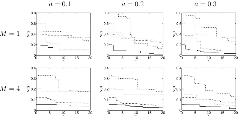
This will always define a process with a Poisson-Dirichlet marginal. Figure (1) shows some

reali-sations of theVtprocess. For comparison, in the Dirichlet process case,Vj(t)would be constant.

a= 0.1 a = 0.2 a= 0.3

M = 1

0 5 10 15 20 0 0.2 0.4 0.6 0.8 t V(t)

0 5 10 15 20 0 0.2 0.4 0.6 0.8 t V(t)

0 5 10 15 20 0 0.2 0.4 0.6 0.8 t V(t)

M = 4

0 5 10 15 20 0 0.1 0.2 0.3 0.4 t V(t)

0 5 10 15 20 0 0.1 0.2 0.3 0.4 t V(t)

0 5 10 15 20 0 0.1 0.2 0.3 0.4 t V(t)

Figure 1:Four realisations ofVj(t)for different values ofaandMin the Poisson-Dirichlet process withλ= 1.

The effect of the Poisson-Dirichlet extension is to discount the value ofVj(t)over time. As the

weights of atoms are built up using factors(1−Vj(t))for the atoms that were introduced earlier,

this leads to larger probabilities for atoms that were introduced in the past than under the Dirichlet

a= 0 a= 0.1 a = 0.2 a= 0.3

M = 1

0 5 10 15 20 0 0.2 0.4 0.6 0.8 1

0 5 10 15 20 0 0.2 0.4 0.6 0.8 1

0 5 10 15 20 0 0.2 0.4 0.6 0.8 1

0 5 10 15 20 0 0.2 0.4 0.6 0.8 1

M = 4

0 5 10 15 20 0 0.2 0.4 0.6 0.8 1

0 5 10 15 20 0 0.2 0.4 0.6 0.8 1

0 5 10 15 20 0 0.2 0.4 0.6 0.8 1

0 5 10 15 20 0 0.2 0.4 0.6 0.8 1

Figure 2:The autocorrelation function for various choice ofaandMfor a fixed value ofλ

we generate larger autocorrelations for past shocks. This effect is illustrated by the shape of the

autocorrelation function shown in Figure 2, which gives the autocorrelation function for various

values ofM andaand for a fixed value ofλ. Larger values ofaleads to increasingly slow decay

of the autocorrelation function for fixedM. Larger values ofM for fixedalead to non-neglible

autocorrelation at longer lags (as with the Dirichlet Process AR which corresponds toa= 0).

a= 0 a= 0.1 a = 0.2 a= 0.3

C = 2

0 5 10 15 0

1000 2000 3000 4000

0 5 10 15 0

1000 2000 3000 4000

0 5 10 15 0

1000 2000 3000 4000

0 5 10 15 0

1000 2000 3000 4000

C = 4

0 5 10 15 0

1000 2000 3000 4000

0 5 10 15 0

1000 2000 3000 4000

0 5 10 15 0

1000 2000 3000 4000

0 5 10 15 0

1000 2000 3000 4000

C = 8

0 5 10 15 0

1000 2000 3000 4000

0 5 10 15 0

1000 2000 3000 4000

0 5 10 15 0

1000 2000 3000 4000

0 5 10 15 0

1000 2000 3000 4000

Figure 3: Number of clusters in 20 draws at time 2 conditional onCclusters in 20 draws at time 1: M = 1and

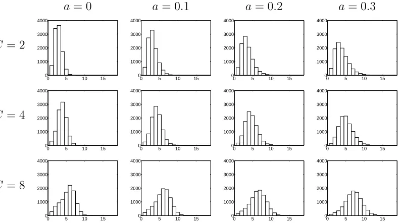
The Poisson-Dirichlet process gives us an extra parameter compared to the Dirichlet process

which is related to the dispersion of the distribution of the number of clusters in a sample of size

kdrawn from the process. Larger values ofaare related to a more dispersed distribution for given

M. In our time series model, the parameteracontrols the number of clusters in a sample of size

kat time tgiven that there wereC clusters at timet−1in a sample of sizek. Figure 3 shows

the distribution fork = 20and various values ofM andC. For a fixed value ofC, the mode of

the distributions seems unchanged by the value ofabut the right-hand tail has more mass on larger

numbers of clusters. This provides the PDAR process with the extra flexiblity (over the Dirichlet

process) to model the process when the number of clusters underlying the data is rapidly changing.

4 Computational methods

We will discuss Markov chain Monte Carlo methods for full sample inference. The MCMC sampler

is defined whena1, a2, . . . andb1, b2, . . . are both nondecreasing sequences. Samplers for

Dirich-let process marginals can be defined using P´olya urn schemes developed in Section 3.1. Samplers

for other marginal processes can be implemented by an extension of the retrospective sampler for

Dirichlet processes (Papaspiliopoulos and Roberts, 2008). Appendix B groups most of the details;

here we specifically focus on introducing latent variables that make Gibbs updating simpler by

ex-ploiting the stick-breaking form ofVj(t)in this case. We assume that the arrival times of the atoms

areτ1 < τ2 < τ3 < . . . and that associated withτj we have sequences²j = (²j,1, ²j,2, . . .) and

wj = (wj,2, wj,3, . . .). We will follow standard methods for stick-breaking mixtures by introducing

latent variabless1, s2, . . . , snthat allocate each observations to one of the atoms. We defineri by

τri = max{τj|τj < ti}. Then, ifti> τj,

p(si =j) =pj(ti) =Vj(ti) ri

Y

k=j+1

(1−Vk(ti))

=





mj_X(ti)+1

l=1

²_j,l(1−w_j,l)

mj_Y(ti)+1

h=l+1

w_j,h



 ri

Y

k=j+1 



mk_X(ti)+1

l=1

(1−²_k,l)(1−w_k,l)

mk_Y(ti)+1

h=l+1

w_k,h



This form is not particular helpful for simulation of the posterior distribution but we define a more

convenient form by introducing latent variablesφas follows

p(φ_ijk =l) = (1−w_k,l)

mk_Y(ti)+1

h=l+1

w_k,h, 1≤l≤mj(ti) + 1, 1≤i≤n, 1≤j≤k≤ri

and

p(si =j|φ) =²j,φijj

ri

Y

k=j+1

(1−²k,φijk).

In effect, each stick-break is a mixture distribution and the indicatorsφchoose components of that

mixture distribution. Then

p(s, φ) =

n Y

i=1 

_²s

i,φ_isisi

ri

Y

k=si+1

(1−²_k,φ

isik)



Yn i=1

ri

Y

j=si

ri

Y

k=j 

_(1−wk,φ

ijk)

mj_Y(ti)+1

h=φijk+1

w_k,h



_.

which is a form that will be useful for simulation of the full conditional distributions ofw and²

which will be beta distributed.

Further details on the MCMC algorithms proposed here are contained in Appendix B.

5 Empirical Results

5.1 Comparison of MCMC algorithms

We compare the marginal (see Section 3.1) and the general conditional algorithms with Dirichlet

process marginals by analysing two simulated data sets and looking at the behaviour of the chain

for the two parametersλandM. The integrated autocorrelation time is used as a measure of the

mixing of the two chains since an effective sample size can be estimated by sample size divided

by integrated autocorrelation time (Liu 2001). We introduce three simple, simulated datasets to

compare performance over a range of possible data.

In all cases, we make a single observation at each time point fort = 1,2, . . . ,100. The data

sets are simulated from the following models. The first model has a single change point at time 50

p(yi) =   

 

N(−20,1) ifi <50

M λ

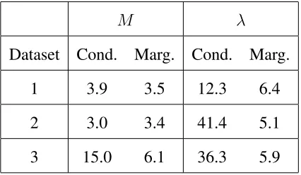
Dataset Cond. Marg. Cond. Marg.

1 3.9 3.5 12.3 6.4

2 3.0 3.4 41.4 5.1

3 15.0 6.1 36.3 5.9

Table 1:The integrated autocorrelation times forM andλusing the two sampling schemes

The second model has a linear trend over time

p(yi) =N µ

40(i−1)

99 −20,1

¶

The third model has a linear trend before time 40 and then follows a mixture of three regressions

after time 40

p(y_i) =

  

 

N

³ 40(i−1)

99 −20,1 ´

ifi <40

3 10N

³ 40(i−1)

99 −20,1 ´

+2₅N(−4,1) + ₁₀3N

³

12−40(₉₉i−1),1

´

ifi≥40. .

These data sets are fitted by a mixture of normals model

yt∼N(µt,1)

µt∼Gt

Gt∼DP AR(M, H;λ).

whereH(µ) = N(µ|0,100). Table 1 shows the results for the three data sets, using Exponential

priors with unitary mean forM andλ. The mixing ofλis much better using the marginal sampler

for each dataset (particularly data sets 2 and 3). The mixing ofMis similar for the first two datasets

but better for dataset 3. Thus, we use the marginal algorithm for the DPAR model in the following

examples.

5.2 Real data examples

We consider three types of example. The first involves a long, single time series taken from the

distri-bution and the other two involve a short panel of many time series. In the latter cases we model the

data through nonparametric mixtures of normal distributions. Throughout, the parametersM andλ

were given exponential prior distributions with mean one.

5.2.1 Financial time series

Financial time series often show a number of stylized features such as heavy tails and volatility

clustering (seee.g. Tsay 2005). Building models with stochastic volatility is a popular method for

capturing these features. A stochastic volatility model assumes that the conditional variance follows

a stochastic process. Ify1, y2, . . . , yT are the observations then a typical discrete time specification

assumes that

yt= p

ht²t

where²_tare i.i.d. from some returns distribution and the conditional varianceh_tis modelled by

loght∼N(α+δloght−1, σ2v).

The distribution of²t is usually taken to be normal. However, financial time series often contain

large values which may not be fully explained by the time-varying variance. This has motivated

the use of other choices. Jacquieret al (2004) considered usingt-distributions. Jensen and

Ma-heu (2007) consider a full Bayesian nonparametric model and show that the return distribution for

an asset index may not be well-represented by either normal or tdistributions. They model the

returns distributions with a Dirichlet process mixture of normals. We extend the model by allowing

the returns distribution to change over time. The hierarchical model can be written as

y_t

√

ht

∼N(µt, σt2)

loght∼N(δloght−1, σ2v)

(µ_t, σ_t2)∼G_t

G_t∼DP AR(M, H;λ).

where H¡µ, σ−2¢ = N(µ|0,0.01σ2)Ga¡σ−2¯¯1,0.1¢ and Ga(x|α, β) represents a Gamma dis-tribution with shapeαand meanα/β. The parametersδ, σ2

relevant ranges:σ−_v2 ∼Ga(1,0.005/2)andδ∼N(0,10)truncated to [0,1] as described in Jacquier

et al(2004). Jensen and Maheu (2007) describe computational methods for the Dirichlet

process-based model which can be extended using the method in Section 3.1. The method is applied to the

daily returns of the Standard & Poors index from January 1, 1980 to December 30, 1987, as shown

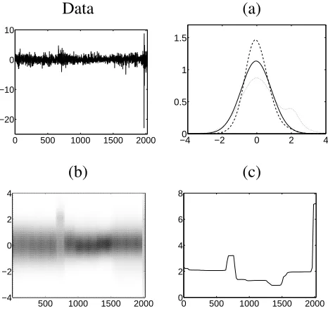
in Figure 4.

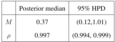
Posterior median 95% HPD

M 0.37 (0.12,1.01)

ρ 0.997 (0.994, 0.999)

Table 2: Posterior inference for some parameters of the model

Posterior inference about the parameters of the model are shown in Table 2. The posterior

me-dian ofM is around 0.37 indicating the nonparametric distribution has two or three normals which

have non-neglible mass and the autocorrelation at 1 lag, ρ, is large showing that the distributions

do not change rapidly over time. The posterior inference for the distributions is shown in Figure 4.

As suggested by the estimates ofM andρwe have results that would be roughly consistent with a

changepoint analysis where several regions with very similar returns distributions have been

identi-fied. Figure 4(b) shows representative distributions for the main periods and illustrates the range of

shapes in the returns distribution. The main difference between the distributions is their spread and

the variance of the fitted distributions is shown in Figure 4(c). The results are extremely smooth

and can be thought of as representing an estimate of underlying, long-run volatility (since daily

changes in volatility are captured through the volatility equation). A parametric analysis assuming

that the returns distribution is normal leads to an estimate of the long-run variance to be 1.66 which

is roughly an average of our nonparametric estimates.

5.2.2 Income data

The data contain the real (log) per capita GDP of 110 EU regions from 1977 to 1996 and has been

previously analysed by Grazia Pittau and Zelli (2006). We ignore the longitudinal nature of the

Data (a)

0 500 1000 1500 2000 −20

−10 0 10

−40 −2 0 2 4 0.5

1 1.5

(b) (c)

500 1000 1500 2000 −4

−2 0 2 4

0 500 1000 1500 2000 0

2 4 6 8

Figure 4:Inference for the Standard & Poors data set: (a) selected predictive density functions for observables at

times 481, 681 and 1181; (b) heatmap of the predictive density functions of the returns at each time point (darker

colours represent higher density values); (c) variance of the fitted returns distribution over time

measurements and model

y_it ∼N(µ_it, σ_it2)

(µit, σit2)∼Gt

Gt∼DP AR(M, H;λ) (7)

whereH¡µ, σ−2¢_=N(µ|µ

0,0.01σ2)Ga ¡

σ−2¯¯_1,0.1¢_{. The hyperparameterµ0represents an}

over-all mean value for the data and the sample mean is adopted as a suitable value. Results are presented

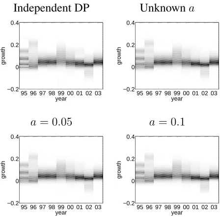
in figure 5. Panel (a) shows a heatmap of the estimated distribution plotted at each year. The most

striking feature of the plots is that the distribution changes from year 1988 to 1989 with larger

values observed from 1989 onwards. It is clear the model very much behaves like a change-point

model with one change-point. Panel (b) shows the estimated densities for each year. The change in

the main model of the data is obvious but there is also a change in the modality of the data and the

shape of the tails. To check whether this change in distribution is supported by the data, we fitted

(a) (b) (c)

1980 1985 1990 1995 8.5

9 9.5 10

8 9 10 11 0

2 4 6

8 9 10 11 0

2 4 6

Figure 5: Income data: (a) heatmap of the estimated distribution for each year using a DPAR mixture model;

(b) density estimates for each year using DPAR; (c) density estimates for each year using independent Dirichlet

process mixture models (pre-1989 shown in light grey and other years in black).

and support the two main distributions inferred from the data. In fact, the yearly distributions are

very similar for the second period (post-1988). It is interesting to note that the density estimates

are much smoother for the independent compared to the DPAR model, which is due to the smaller

amount of information available for each estimate.

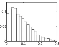
5.2.3 NUTS data

0 0.1 0.2 0.3 0

0.05 0.1

Figure 6: Posterior distribution ofafor the NUTS data

The data consists of annual per capita GDP growth rates for 258 NUTS2 European regions

covering the period from 1995 to 2004 (NUTS2 regions provide a roughly uniform breakdown

of the EU into territorial units). The data are modelled using a mixture of normal distributions

as in model (7) with the exception that now we use the model with Poisson-Dirichlet marginals:

Gt ∼PDAR(a, M, H;λ). We consider the cases whereais fixed and whereais given a uniform

Independent DP Unknowna

95 96 97 98 99 00 01 02 03 −0.2

0 0.2 0.4

year

growth

95 96 97 98 99 00 01 02 03 −0.2

0 0.2 0.4

year

growth

a= 0.05 a = 0.1

95 96 97 98 99 00 01 02 03 −0.2

0 0.2 0.4

year

growth

95 96 97 98 99 00 01 02 03 −0.2

0 0.2 0.4

year

growth

Figure 7:Heatmaps of the fitted yearly distribution of growth for the NUTS data

Figure 6 shows the posterior distribution of a, which places its mass on smaller values of a

(under 0.3) with mode around 0.05. The yearly predictive distribution of growth is shown in figure 7

for the PDAR witha = 0.05anda = 0.1andaunknown. This figure also presents results for a

model where the distribution of each year’s growth is estimated independently with a Dirichlet

process mixture. The results are remarkably consistent across all models. This is perhaps not

surprising since we are looking at posterior means with a substantial amount of data in the sample

and large differences between each year’s distribution. When the data is thinned at random to a

Independent DP a= 0.05

95 96 97 98 99 00 01 02 03 −0.2

0 0.2 0.4

year

growth

95 96 97 98 99 00 01 02 03 −0.2

0 0.2 0.4

year

growth

Figure 8: Heatmaps of the fitted yearly distribution of growth for the thinned NUTS data

sample of 60 regions over 9 years, Figure 8 contrasts the results for independent DP and the PDAR

when distributions in consecutive years are similar, as we would expect from a “change-point”

type analysis. However, even with the full data set there are differences between the posterior

distributions of the parameters of the model. Figure 9 shows the posterior distribution ofλ. This is

Unknowna a = 0.05 a = 0.1

0 2 4 6

0 0.05 0.1 0.15 0.2

0 2 4 6

0 0.05 0.1 0.15 0.2

0 2 4 6

0 0.05 0.1 0.15 0.2

Figure 9: Posterior distribution ofλfor the NUTS data

the mean number of new clusters introduced each year. The distribution is concentrated between 2

and 4. Once again, this indicates the large differences between the distributions for each year. The

mean ofλis 2.69 whena= 0.05and 2.98 whena= 0.1. Whenais unknown the mean, 2.87, falls

between these two values. As we increaseain the Poisson-Dirichlet model then we are more likely

to introduce smaller components which allows the introduction of larger numbers of components at

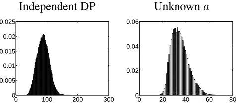
each year. This idea is supported by the posterior distribution of the number of clusters: the median

Independent DP Unknowna

0 100 200 300 0

0.005 0.01 0.015 0.02 0.025

0 20 40 60 80 0

0.02 0.04 0.06

Figure 10:Posterior distribution of the number of clusters for the NUTS data

number of clusters is 32 ifa= 0.05and 36 ifa= 0.1. Whenais unknown the median number of

clusters is 34. Figure 10 displays its posterior distribution and also presents the posterior distribution

of the number of clusters when we model the data in each year with independent Dirichlet process

mixture models. In the latter case we obtain a substantially larger number of clusters (the median is

that despite the lack of similarity between the distribution of each year some clusters can usefully

be carried over from one year to the next.

6 Discussion

This paper introduces, develops and implements inference with a new class of time-dependent

measure-valued processes with stick-breaking marginals, which can be used as a prior

distribu-tion in nonparametric time-series modelling. The Dirichlet process and Poisson-Dirichlet process

marginals arise as natural special cases. We derive a P´olya urn scheme for the Dirichlet process case

which allows us to develop a new algorithm using a marginalised method. This method typically

leads to better mixing of the parameter (particularly the intensity parameter of the Poisson process).

We also develop a conditional simulation method using retrospective sampling methods when the

parameters of the stick-breaking process are nondecreasing.

Moving from Dirichlet process to Poisson-Dirichlet process marginals allows us to more closely

control the conditional distribution of the number of clusters in a sample of sizenat timetgiven

the number at timet−1. The processes provide smoothed estimates of the distributions of interest.

The models can behave like a change point model which allows the discovery of periods where

distributions are relatively unchanged.

References

Antoniak, C. E. (1974): “Mixtures of Dirichlet processes with applications to non-parametric

problems,”Journal of the American Statistical Association, 2, 1152-1174.

Carlin, B. P., A. E. Gelfand and A. F. M. Smith (1992): “Hierarchical Bayesian analysis of

change-point problems,”Applied Statistics, 41, 389-405.

Caron, F., M. Davy and A. Doucet (2007): “Generalized P´olya Urn for Time-varying Dirichlet

Process Mixtures”,23rd Conference on Uncertainty in Artificial Intelligence (UAI 2007).

De Iorio, M., P. M¨uller, G. L. Rosner and S. N. MacEachern (2004): “An ANOVA model for

Doucet, A., N. de Freitas and N. J. Gordon (2001): “Sequential Monte Carlo Methods in Practice,”

Springer-Verlag: New York.

Dunson, D. B. (2006): “Bayesian dynamic modeling of latent trait distributions,”Biostatistics, 7,

551-568.

Dunson, D. B., N. Pillai and J. H. Park (2007): “Bayesian density regression, ”Journal of the

Royal Statistical Society B, 69, 163-183.

Grazia Pittau, M. and R. Zelli (2006): “Empirical Evidence of Income Dynamics Across EU

Regions,”Journal of Applied Econometrics, 21, 605-628.

Griffin, J. E. (2007): “The Ornstein-Uhlenbeck Dirichlet Process and other time-varying

pro-cesses for Bayesian nonparametric inference,” Working Paper 07-03, CRiSM, University of

Warwick.

Griffin, J. E. and M. F. J. Steel (2006): “Order-based Dependent Dirichlet Processes,”Journal of

the American Statistical Association, 101, 179-194.

Ishwaran, H. and L. F. James (2001): “Gibbs Sampling Methods for Stick-Breaking Priors,”

Jour-nal of the American Statistical Association, 96, 161-173.

Ishwaran, H. and L. F. James (2003). “Some further developments for stick-breaking priors: finite

and infinite clustering and classification,”Sankhya, A, 65, 577-592.

Ishwaran, H. and M. Zarepour (2000): “Markov chain Monte Carlo in approximate Dirichlet and

two-parameter process hierarchical models,”Biometrika, 87, 371-390.

Jacquier, E., N. G. Polson and P. E. Rossi (2004): “Bayesian analysis of stochastic volatility

models with fat tails and correlated errors,”Journal of Econometrics, 122, 185-212.

James, L.F. (2008): “Large sample asymptotics for the two-parameter PoissonDirichlet process,”

in Pushing the Limits of Contemporary Statistics: Contributions in Honor of Jayanta K.

Ghosh, B. Clarke and S. Ghosal, eds., IMS: Beachwood, 187-199.

James, L. F., A. Lijoi and I. Pr¨unster (2005): “Bayesian inference via classes of normalized random

Jensen, M. J. and J. M. Maheu (2007): “Bayesian semiparametric stochastic volatility modeling,”

Technical Report, University of Toronto.

Liu, J. S. (2001):Monte Carlo Strategies in Scientific Computing, Springer-Verlag: New York.

Lo, A. Y. (1984): “On a Class of Bayesian Nonparametric Estimates: I. Density Estimates,”The

Annals of Statistics, 12, 351-357.

M¨uller, P., F. Quintana, and G. Rosner (2004): “A method for combining inference across related

nonparametric Bayesian models,”Journal of the Royal Statistical Society B, 66, 735-749.

Nieto-Barajas, L., M¨uller, P., Ji, Y., Lu, Y. and Mills, G. (2008): “Time Series Dependent Dirichlet

Process,”Preprint

Papaspiliopoulos, O. and G. Roberts (2008): “Retrospective MCMC for Dirichlet process

hierar-chical models,”Biometrika, 95, 169-186.

Pitman, J. (1996): “Some Developments of the Blackwell-MacQueen Urn Scheme,” inStatistics,

Probability and Game Theory: Papers in Honor of David Blackwell, eds: T. S. Ferguson, L.

S. Shapley and J. B. MacQueen, IMS Lecture Notes.

Pitman, J. and M. Yor (1997): “The two-parameter Poisson-Dirichlet distribution derived from a

stable subordinator,”Annals of Probability, 25, 855-900.

Rodriguez, A. and E. ter Horst (2008): “Bayesian Dynamic Density Estimation,”Bayesian

Anal-ysis, 3, 339-366.

Teh, Y. W. (2006): ‘A Hierarchical Bayesian Language Model based on Pitman-Yor Processes,”

Proceedings of the Annual Meeting of the Association for Computational Linguistics 44.

Tsay, R. (2005):Analysis of Financial Time Series (2nd Edition), John Wiley & Sons: New York.

Zhu, X., Z. Ghahramani, and J. Lafferty (2005): “Time-Sensitive Dirichlet Process Mixture

A Appendix

A.1 Proof of Theorem 1

These proofs use the following properties:

1. Suppose thatq ∼ Ga(a)andr ∼Ga(b)are independent thenv = _q+q_r ∼Be(a, b)which is independent ofu=q+r ∼Ga(a+b).

2. If q ∼ Ga(a+b)and independent of v ∼ Be(a, b) thenvq ∼ Ga(a) and independent of

(1−v)q∼Ga(b).

Property 1 implies that any beta random variable,v, can be expressed as _q+q_r where q andr are independent. We can writeVj,t= _qj,tq₊j,t_rj,t, whereqj,t∼Ga(at)andrj,t∼Ga(bt)for all cases.

Case (i) Let qj,t+1 = qj,t +xj,t+1 and rj,t+1 = rj,t +zj,t+1 wherexj,t+1 ∼ Ga(at+1 −at) and

independent of zj,t+1 ∼ Ga(bt+1 −bt). Thenqj,t+1 ∼ Ga(at+1) and rj,t+1 ∼ Ga(bt+1)

andqj,t+1andrj,t+1are independent. ThenVj,t+1 = _qj,t+1qj,t₊+1_rj,t+1 is beta distributed with the

correct parameters. Simple algebra shows that we can write

V_j,t+1= qj,t+1

qj,t+1+rj,t+1

=w_j,t+1V_j,t+ (1−w_j,t+1)²_j,t+1

wherew_j,t+1 = qj,t+rj,t

qj,t+rj,t+xj,t+zj,t and²j,t+1 =

xj,t

xj,t+zj,t. From the property of beta-gamma distributionsxj,t +zj,t is independent of²j,t+1 and it follows that wj,t+1 is independent of

²j,t+1. Finally,wj,t+1 ∼ Be(at+1+bt+1, at+1 +bt+1−at−bt)and²j,t+1 ∼ Be(at+1 −

at, bt+1−bt)

Case (ii) Then we can writeqj,t+1 =uj,t+1qj,tandrj,t+1 =yj,t+1rj,t whereuj,t+1 ∼Be(at+1, at−

at+1)andyj,t+1 ∼ Be(bt+1, bt−bt+1). Application property 2 shows thatqj,t+1Ga(at+1)

andrj,t+1 ∼Ga(bt+1)are independent and soVj,t+1 = _qj,t+1qj,t₊+1_rj,t+1 is beta distributed with

the correct parameters. This can be re-expressed as follows

Vj,t+1 = _q qj,t+1 j,t+1+rj,t+1 =

wj,t+1Vj,t

wj,t+1Vj,t+ (1−wj,t+1)(1−Vj,t)

wherewj,t+1= _uj,t+1uj,t₊+1_yj,t+1.

Case (iii) Then we can writeqj,t+1=yj,t+1qj,tandrj,t+1=rj,t+zj,t+1whereuj,t+1 ∼Be(at+1, at−

at+1)andzj,t+1∼Ga(bt+1−bt).

Vj,t+1 = _q qj,t+1 j,t+1+rj,t+1 =

uj,t+1qj,t

uj,t+1qj,t+rj,t+zj,t+1.

Case (iv) Then we can writeqj,t+1 =qj,t+xj,t+1andrj,t+1 =yj,t+1rj,twherexj,t+1 ∼Ga(at+1−at)

andy_j,t+1∼Be(b_t+1, b_t−b_t+1).

Vj,t+1= _q qj,t+1 j,t+1+rj,t+1

= qj,t+xj,t+1

A.2 Proof of Theorem 2

Letki = #{i|φi < τi < φi+1}for1≤i≤ln,m−1.

p(k1, k2, . . . , kln,m−1|s1, s2, . . . , sn)∝

ln,m_Y−1

i=1 µ

M M+An(φi+1

¶_ki

(λ(φi+1−φi))ki

which shows that the number of points on(φ_i, φ_i+1)is Poisson distributed with mean

³ M M+An(φi+1

´

λ(φi+1−φi). The position of the points is unaffected by the likelihood and so the

posterior is a Poisson process. There is no likelihood contribution for the intervals(−∞, φ1)and

(φln,m,∞). Since the Poisson process has independent increment then the posterior distribution on these intervals is also a Poisson process with intensityλ.

A.3 Proof of Theorem 3

In order to calculate the predictive distribution we need to calculate the probability of generating the samples1, s2, . . . , snwhich given by

p(s1, s2, . . . , sn) =E[p(s1, . . . , sn|V1, V2, V3, . . . , τ1, τ2, τ3, . . .)].

This expectation can be derived by first noting that

p(s₁, . . . , s_n|V₁, V₂, V₃, . . . , τ₁, τ₂, τ₃, . . .) = Y

i∈R

Vηi

i (1−Vi)An(τi)

whereR={i|min{τsi,1≤i≤n} ≤τi ≤max{ti,1≤i≤n}}. Marginalising overV gives

p(s1, . . . , sn|τ1, τ2, τ3, . . .) = Y

i∈R

M η_i!Γ(M+A_n(τ_i)) Γ(M + 1 +ηi+An(τi)).

Noticing that, ifηi = 0then

M ηi!Γ(M+An(τi))

Γ(M + 1 +ηi+An(τi)) =

M M+An(τi),

it follows that

p(s₁, . . . , s_n|S_n,m) =

kn

Y

i=1

M η_i!Γ(M+A_n(τ? i))

Γ(M+ 1 +ηi+An(τi?)) l_Yn,m

i=2

E

"µ

M M+An(φi)

¶_{#{j|φi−1<τj<φi}}#

.

From Theorem 2,#{j|φ_i−1 < τ_j < φ_i} is Poisson distributed with meanλ

³ M M+An(φi)

´

(φ_i −

φi−1)and so

E

"µ

M M+An(φi)

¶_{#{j|φi−1<τj<φi}}#

= exp

½

−λ(φi−φi−1)

M A_n(φ_i) (M +An(φi))2

and

p(s1, . . . , sn|Sn,m) = kn

Y

i=1

M ηi!Γ(M+An(τi?))

Γ(M + 1 +η_i+A_n(τ? i))

l_Yn,m

i=2

exp

½

−λ(φi−φi−1)_(MM A_+An(φi) n(φi))2

¾

it also follows that ifsn+1 =jwherej≤knthen, ifm≥n+ 1,

p(s1, . . . , sn, sn+1 =j|Sn,m) =M(ηj+ 1)!Γ(M +An(τ ? i))

Γ(M+ 2 +ηj+An(τi?)) kn

Y

i=1;i6=j

M ηi!Γ(M+An+1(τ_i?))

Γ(M+ 1 +ηi+An+1(τi?))

×

l_Ym,n

i=2

exp

½

−λ(φ_i−φ_i−1)

µ

M M+An(φi)

¶

A_n+1(φ_i)

M+An+1(φi) ¾

.

So that, ifj≤kn,

p(sn+1 =j|Sn,m, s1, . . . , sn) = p(s1, . . . , s_p(s n, sn+1 =j|Sn,m) 1, . . . , sn|Sn,m)

;

after some algebra we get the form in the Theorem. Otherwise,sn+1 = kn+ 1 and we need to

calculatep(s1, . . . , sn, sn+1=kn+ 1, τ_k?_n+1 ∈(φi−1, φi)|Sn,m). It is clear that

M ηi!Γ(M+An+1(φi))

Γ(M+ 1 +ηi+An+1(φi)) =        M

M+An(φi) ifφi−1 < τi < τ

? kn+1

M

(M+An(φi))(M+1+A+n(φi)) ifτi =τ

? kn+1

M

M+An(φi)+1 ifτ

?

kn+1< τi< φi

.

Letτkn−1 = (1−w)φi+wφi−1,

E

" µ

M M +An+1(φi)

¶_{#{j|φi−1<τj<φi}}¯_¯ ¯ ¯

¯τk?n+1,#{j|φi−1 < τj < φi}=k

#

= M

(M +An(φi))(M+ 1 +An(φi))

k

·

M M+An(φi) + 1

w+ M

M +An(φi)

(1−w)

¸_k−1

and so

E

" Ã

M M +An+1(φi)

#{j|φi<τj<φi+1}

!¯ ¯ ¯ ¯ ¯τ ? kn+1

#

= M

(M +An(φi))(M+ 1 +An(φi))

×λM(φi−φi−1)

M+An(φi) ·

exp

½

−λM(φi−φi−1)

M+An(φi) ·

An(φi) + 1

M +An(φi) + 1w+

An(φi)

M +An(φi)(1−w) ¸¾¸

.

Finallyτ?

kn+1is uniformly distributed on(φi−1, φi)which implies that E

"Ã

M M+An(φi)

#{j|φi−1<τj<φi}

!#

= exp

½

−M λ(φi−φi−1)An(φi)

(M +An(φi))2

¾ ·

1−exp

½

− M

2_λ(φ

i−φi−1)

(M +An(φi))2(M+An(φi) + 1) ¾¸