Int. J. Nanosci. Nanotechnol., Vol. 14, No. 1, March. 2018, pp. 71-83
Short Communication
Statistical Modeling for Oblique Collision of
Nano and Micro Droplets in Plasma Spray
Processes
H. Panahi1,* and S. Asadi2 1
Department of Mathematics and Statistics, Lahijan branch, Islamic Azad University, Lahijan, Iran.
2
Department of Mechanical Engineering, Payame Noor University (PNU), P.O. Box: 19395-3697, Tehran, Iran.
(*) Corresponding author: [email protected]
(Received: 12 February 2016 and Accepted: 03 August 2016)
Abstract
Spreading and coating of nano and micro droplets on solid surfaces is important in a wide variety of applications including plasma spray coating, ink jet printing, DNA synthesis and etc. In spraying processes, most of droplets collide obliquely to the surface. The purpose of this article is to study the distribution of nano and micro droplets spreading when droplets impact at an oblique angle. We introduce the generalized exponential distribution as a new alternative for spreading data. The generalized exponential distribution shares many physical properties of the Weibull distribution which is used frequently for engineering data. For shape parameter greater than one, the generalized exponential distribution offers increasing hazard function, which is in accordance with the inclined droplet impact in plasma coating processes. We apply a number of criteria and model selection tests to evaluate the suitability of the generalized exponential distribution to other rival models, such as the Weibull, inverse Weibull, Burr III, Burr X, inverted exponentiated Rayleigh and exponentiated Pareto distributions. The analyses results indicate that the generalized exponential distribution shows better results than the other distributions for nano and micro droplets spreading data. Finally, graphical displays for informal checks on the appropriateness of the generalized exponential distribution in probabilistic assessment of inclined impact as well as formal goodness of tests are presented. An important implication of the present study is that the generalized exponential distribution, in contrast to other distributions, fits more appropriately in the spreading data.
Keywords: Generalized exponential distribution, Model selection procedures, Oblique collision, Plasma spray, Nano and micro droplets.
1. INRODUCTION
Plasma spray coating could be a method by that the extreme temperature of a plasma is utilized to melt powders of metallic or non-metallic materials and spray them onto a solid surface, forming a dense thin layer. The method is typically used to apply protective coatings on parts to protect them from corrosion, erosion and high temperatures. Coating layer is shaped by impact and spreading of droplets
micro- droplets and splat formation in plasma spray studies can be generally categorized into one of two researches:
modeling of oblique impact by numerical analysis or morphology of splats.
Although the droplets usually impact upon a surface obliquely in real situations, few studies on the oblique droplet impact are found in literature. Kang and Lee [4] studied the dynamic behavior of a water droplet impinging upon a heated surface. Their results showed that droplet behavior after impact was greatly influenced by the normal momentum of the impinging droplet. Kang and Ng [5] estimated the effects of the angle of impact on the splat
final morphology and spreading behavior. Their paper presented the spread factors and aspect ratios of individual splats at different substrate inclinations. Asadi et al. [1] studied the inclined impact of a droplet on a solid surface in a plasma spray coating process using both numerical and analytical models. They predicted the droplet impact behavior. Asadi and Passandideh-Fard [6] studied the impingement of a droplet onto a thin liquid 0.0 s
0.2 s
0.4 s
0.8 s
2.0 s
Top view Figure 1. Images (3D view and top view) of a zirconium droplet impacting on a solid surface in a plasma coating process. [1]
film by numerical simulation. They found that the dynamic processes after impact are sensitive to the initial droplet velocity and the liquid pool depth. They developed simple expression that correlate the non-dimensional parameters involved in the droplet impingement onto a thin liquid film. Asadi [7] developed a novel computational fluid dynamics and molecular kinetic theory (CFD-MK) method for simulation of a nanodroplet impact onto a solid surface. The author analyzed the spreading behavior for the wettable, partially wettable and nonwettable surfaces. Randive et al. [8] discussed the implications of wall wettability and inclination of the surface on droplet dynamics. They observed that the effect of inclination of the surface on droplet dynamics is more pronounced on a hydrophobic surface as compared to a hydrophilic surface. Jina et al. [9] studied the effects of droplet size and surface temperature on the impact, freezing, and melting processes of a water droplet on an inclined cold surface. They found that the increase of droplet size led to the increases of spreading time, spreading maximum diameter, gliding maximum diameter, and maximum displacement of foremost point. Aboud and Kietzig [10] applied oblique drop impacts which were performed at high speeds with mill metric water droplets. They applied a linear model to define the oblique splashing threshold. LeCleara et al. [11] discussed the dynamic behavior of water drops impacting on inclined superhydrophobic surfaces. Their results suggest that the Weber numbers, based on the velocity components, affect the impact dynamics of a drop such as the degree of drop deformation as long as the superhydrophobicity remains intact.
However, in all previous studies the most attention has been targeted on the dynamics of droplet impact or splat morphology. A literature survey carried out by the author indicated lack of published information on nano and micro
droplets oblique impact analyzing by statistical distributions.
In the present paper, we analyze the data of nano and micro droplets oblique impact as obtained in Kang literatures [4, 5]. Although the Weibull distribution function is widely used to model or characterize the engineering data, but this distribution has certain drawback. For instance, the distribution of the mean of independent and identically distributed Weibull random samples is difficult to obtain. In addition, the Weibull distribution with shape parameter greater than one cannot be used for many engineering data. Therefore, we often end up with situations where studying of other statistical distributions may be required. Gupta and Kundu [12] observed that the generalized exponential (GE) distribution can be used quite effectively to analyze several lifetime data in place of Weibull distribution. It has a nice physical interpretation. However, no study has been carried out to date to show the suitability of the GE distribution in the spreading data. So, the main aim of this paper is to develop the different model selection tests and graphical methods for investigating the efficiency of the GE distribution in spreading data.
2. DIFFERENT RIVAL MODELS In this section, we briefly describe different rival models and estimate the unknown parameters of them using a samplex( ,...,x1 xn).
2.1. Generalized Exponential Distribution
biological research. Several applications of the GE distribution can be found in Pasari and Dikshit [13], Panahi and Asadi [14] and Gupta and Kundu [15]. The GE distribution for 0and 0has the following density function:
1
( ; , ) x(1 x) , 0
GE
f x e e (1)
Here and are the shape and scale parameters respectively. Therefore, the maximum likelihood estimators (MLEs) of and can be obtained by maximizing the following log-likelihood function with respect to the unknown parameters;
1 1
( , ) ln( ) ln( )
ln( ) ( 1) ln(1 i)
GE
n n
x i
i i
L data n n
x e
(2) The MLEs of and , say ˆ and ˆ respectively can be obtained as the solutions of1
(1 i) 0
n
x i
L n
Ln e
(3)and
1 1
ln 1 0
1 i i x n n i i x i i
L n x e
x e
(4)From (3), we have
ˆ 1
ˆ
ln(1 i)
n x i n e
(5) A simple manipulation of (4) gives rise to the equation (6) in terms of a single variable, which can be easily solved numerically or using any standard software packages such as R.ˆ
1 1
1
ln ( 1) 0
1 ln(1 ) i i i x n n i
i n x
x
i i
i
n n x e
x e e
(6) Alternatively, we can estimate directly from (2) by maximizing1
1 1
ˆ
( ) ( , ) ln ln(1 )
ln ln(1 )
i i n x GE i n n x i i i
g L n e
n x e
(7)It is observed that the gGE( ) is unimodal. Thus, we can find the maximum likelihood estimates, by differentiating gGE( ) with respect to and then equating to zero. We have 1 1 1 1 /(1 ) ( ) ln(1 ) 0 1 i i i i i n x x i i GE n x i x n n i i x i i
n x e e
g e x e n x e
(8) Equation (8) can be solved using different numerical techniques such as Newton-Raphson algorithm or by using any standard one-dimensional non-linearequation solver package. For
completeness, we have provided the Newton-Raphson algorithm as
1
( )
; 1,2,... ( ) i i i i g i g (9) For solution the above iterative procedure, we guess an initial value(0)
and continue the iterative procedure when
( 1)i ( )i
. Once we get the MLE of the MLE of can be obtained from (5).
2.2. Burr Type X Distribution
Burr [16] introduced twelve different forms of cumulative distribution functions for modeling data. Among those twelve distribution functions, Burr Type X, Burr Type XII and Burr Type III received the maximum attention. Several aspects of the Burr Type X and Burr Type XII distributions were studied by several authors [17-22]. The Burr Type X (BX) distribution has the probability density function (PDF) for x0as
2 2
2 ( ) ( ) 1
( ; , ) 2 x (1 x ) , 0
BX
f x x e e
2
( ) 2 2
1 1 1
( , ) ln( ) 2 ln( )
ln( ) ( 1) ln(1 i )
BX
n n n
x
i i
i i i
L data n n
x x e
(11) with respect to the and . So, if ˆ andˆ
are the MLE of and respectively, then 2 ˆ ( ) 1 ˆ
ln(1 i )
n x i n e
(12) Similarly, the MLE of can be obtained by maximizing the following profile log-likelihood function as2 2 ( ) 1 ( ) 2 2 1 1 ˆ
( ) ( , ) ln ln(1 )
2 ln ln(1 )
i i n x BX i n n x i i i
g L n e
n x e
(13)2.3. Exponentiated Pareto Distribution Pareto distribution is one of the most popular distributions in analyzing the skewed data. This distribution received attention by the researchers due to its broad applications in different fields including, insurance, business, economics, engineering, reliability, hydrology and mineralogy. Moreover, adding one or more parameters to a distribution makes it richer and more flexible for modeling data. Adding a parameter by exponentiation is one of the important ways for adding parameter(s) to a distribution which proposed by AL-Hussaini [23]. By using the proposed cumulative distribution function (CDF), the probability distribution function of the exponentiated Pareto (EPA) can be written as:
1 1
( ; , ) (1 ) (1 (1 ) ) ;
0, 0, 0
EPA
f x x x
x (14)
where and are the shape parameters. Therefore, the MLEs of and can be obtained by maximizing the following log-likelihood function with respect to the unknown parameters as:
1 1
( , ) ln ln
( 1) ln(1 ) ( 1) ln(1 (1 ) ).
EPA
n n
i i
i i
L data n n
x x
(15)Differentiating the log-likelihood function partially with respect to and and equating them to zero, we obtain
1 1
(1 ) ln(1 )
ln(1 ) ( 1) 0,
1 (1 )
n n i i i i i i x x L n x x
(16) and 1ln(1 (1 ) ) 0.
n i i L n x
(17)Note that,
1
ˆ
ln(1 (1 ) )
n i i n x
(18)and the MLE of can be obtained by solving
1
1 1
1
( ) ln ln ln(1 (1 ) )
( 1) ln(1 ) ( 1) ln(1 (1 ) ). ln(1 (1 ) )
n
EPA i
i
n n
i n i
i i
i i
g n n x
n x x x
(19)2.4. Weibull Distribution
The Weibull (WE) distribution is one of the most popular distributions in analyzing the lifetime data. Due to its practicality, it can be used for many applications. Since then, several authors have discussed its properties in a wide range of applications [24,25]. The Weibull distribution with the shape parameter of 0and scale
parameter of 0has the probability density function as;
1
( ; , ) x 0 , 0
WE
f x xe (20)
Here and represent the shape and scale parameters respectively. The MLE of and can be obtained by maximizing the log- likelihood function
1 1 , 1 ln W E n n i i i iL data nLn nLn
x x
with respect to the unknown parameters. Therefore, if ˆ and ˆare the MLE of and respectively, then
1 ˆ n i i n x
(22) Furthermore, the MLE of can be obtained by maximizing the profile log-likelihood of .2.5. Inverse Weibull Distribution
The Inverse Weibull (IWE) distribution is the popular distributions in analyzing the data with both the monotone and unimodal hazard function. The IWE with the shape parameter of 0and scale parameter of
0
has the probability density function as:
1
( ; , ) x 0 , 0
IWE
f x x e (23)
The quantities of 0 and 0 are the shape and scale parameters, respectively. The log-likelihood function of the observed data can be written as:
1 1 , 1 ln IW E n n i i i iL data nLn
nLn x x
(24) By differentiating the log-likelihood function with respect to and and equating the resulting terms to zero, the equation can be written as:1 ˆ n i i n x
(25) Moreover, the MLE of can be obtained by maximizing the above equation to:
1 1
( ) 1 ln
n n
IWE i i
i i
g nLn nLn x x
(26)
2.6.Inverted Exponentiated Rayleigh The Inverted Exponentiated Rayleigh (IER) distribution has been used quite effectively in analyzing various skewed lifetime data. This distribution is usually considered as an alternative model to
lognormal, inverse Weibull and
generalized inverted exponential distribution because of similar distributional properties. The probability distribution function of the IER can be written as:
2 2
3 / / 1
( ; , ) 2 (1 ) ;
0 , 0
x x
IER
f x x e e
(27)
The MLE of and can be obtained by maximizing the log- likelihood function
/ 22
1 1
,
1 ln(1 i )
IER
n n
x
i i i
L data nLn nLn
e x
(28) By differentiating the natural logarithm of the likelihood function with respect to and and equating the resulting terms to zero, we get2
/ 2
1 1
1
ln(1 i ) 0
n n x i i i n e x
(29) 2 / 1ln(1 i )
n x i n e
(30) The MLE of can be obtained using the similar method.2.7. Burr Type III Distribution
The Burr Type III (BIII) distribution is one of the most popular distribution in analyzing the real data [26,27]. The probability distribution function of the BIII is given by
1 ( 1)
( ; , ) (1 ) , 0
BIII
f x x x (31)
Here, and are two shape parameters. The MLE of and say ˆ
and ˆcan be obtained similarly.
3. DIFFERENT MODEL SELECTION PROCEDURES
In this section we describe different available criteria for choosing the best fitted model to a given dataset. Suppose there are two families which are,
(.), p
( )F f R f , G
g(.),Rq
( )g .following criteria can be used for model selection.
3.1. Akaike’s Information Criterion Consider a sample of independently identically distributed (i.i.d.) random variables,X1,...,Xn having probability
density function of h(.)h. The Kullback-Leibler (KL) information in favor of h against f is defined as:
( ) ( )
( , ) log ( ) log
( ) ( )
h
h X h x
KL h f E h x dx
f X f x
(32)
( , ) 0
KL h f and KL h f( , ) 0 , implies thath f. The KL divergence is often intuitively interpreted as a distance between the two probability measures, but this is not mathematically a distance; in particular, the KL divergence is not symmetric. The Akaike [28] introduced the Akaike information criterion (AIC) to select the best model under parsimony. The goal of AIC is to minimize the KL divergence of the selected model from the true model. Notice that the relevant part of the KL divergence is Eh(log f (X))
which
has an estimator as:
ˆ
1 1
log n( )
n
i i
f x
n
(33) where, ˆn ( ˆn, ˆn)is the maximum likelihood estimator (MLE) of ( , ) . It can be considered as an estimator of the divergence between the true density and the model. Akaike introduced his criterion to model selection as:ˆ
1 ˆ
( ) 2 log n( ) 2
n f
n i
i
AIC f x p
(34)where, p is the number of parameters in the model. Now choose the family F if
f g
AIC AIC and choose family G
otherwise.
3.2. Bayesian Information Criterion A popular alternative model selection criterion is the Bayesian information criterion (BIC) which is defined as [29]:
ˆ
1 ˆ
( ) 2 log n( ) log
n f
n i
i
BIC f x p n
(35)where, p and n are the number of parameters and sample size respectively. The most well-known properties of BIC are asymptotic optimality and consistency.
We choose family F if f g
BIC BIC ;
otherwise we choose family G.
3.3. Kolmogorov- Smirnov (K-S) Distance
The K-S distance is one of important distances between two cumulative distribution functions which belongs to the family of non-parametric and distribution- free goodness-of-fit tests. For computing the K-S test, we first construct the empirical distribution function for i.i.d. random variables X1,...,Xnas:
1 1 ( )
i n
n X x
i
F x I
n
(36)where, IXix is the indicator function as:
1
0 otherwise i
i
X x
X x
I
(37) Now, the corresponding K-S distances are calculated as:
sup ( ) ( )
F n
x
D F x F x
(38)
sup ( ) ( )
G n
x
D G x G x
(39) To implement this procedure, a candidate from each parametric family that has the smallest K-S distance should be found and then the different best fitted distributions should be compared.
3.4. The Total Time on Test (TTT) Transform
In many applications, there is qualitative information about the failure rate function shape, which can help in choosing a best model. The TTT transform is a very good idea about the shape of the hazard function of a distribution. The TTT transform of a probability distribution with absolutely continuous distribution function F(.) is given by
1 1
( ) ( ) / (1)
F x HF x HF
where,
1( )
1
0
( ) F x 1 ( ) ; 0 1
F
H x F u du u
. Thecorresponding empirical version of the scaled TTT transform is defined as
: 1:
1
1 1
: 1:
1
0:
( 1)( )
( / )
( / ) ;
(1)
( 1)( )
1,..., , 0
i
j n j n
j n
n n
j n j n
j
n
n j x x
H i n
i n
H
n j x x
i n x
(41) It has been shown by Aarset [30] that the TTT transform is convex (concave) if the hazard rate is decreasing (increasing). In addition, for a distribution with bathtub (unimodal) failure rate the scaled TTT transform is first convex (concave) and then concave (convex).
3.5. The Chi-Square Test
The chi-square test is the one of the oldest method which is being used for goodness of fit. This test uses the observed (Oi) and expected frequencies (Ei) of class
intervals to calculate the chi-square value. For computing, initially the sample is divided in k different groups and counted the number of observations in each group. Then, compute the expected number of observations in each group based on the fitted model of F. we obtain the chi-square test between{ ,...,x1 xn} and the best fitted model from the family F as
2 2
,
1
(O )
k
i i
f data
i i
E E
(42) using the results produced by Chernoff and Lehmann [31], they observed that under the null hypothesis, the test statistic converges to a distribution between a chi-square distribution with k-1 degrees of freedom and a chi-square distribution with k-s-1 degrees of freedom, where k is the number of intervals and s is the number of unknown parameters of the fitted model. If the chi-square value does not lie in the critical region at % signification level, then we conclude that the fitted model fits the data reasonably good and hence, it canbe used to obtain inferential results from the considered data set.
4. EXPERIMENTAL RESULTS
In this section, we analyze the data of inclined ultrafine droplets spreading that obtained in Kang [1, 4]. In this data, the spread factor , , is defined as the ratio of splat diameter to droplet diameter, i.e.
/
e p
d D
(43) where, deis the equivalent diameter of the elliptical splat area and Dp is the droplet diameter before impacting on the substrate. The elliptical splat area is converted to an equivalent splat of circular shape so that its equivalent diameter de can be derived.
The spread factor data measured by means of Scanning Electron Microscopy (SEM) and high resolution surface profilometry and reported in 90 substrate inclination angle. Figure 2 shows the SEM images of splats that obtained in Kang and Ng [5].
Figure 2. SEM examination figures that obtained in Kang and Ng [5]. The angles of impact are (a) 10°, (b) 20°, (c) 30°, (d) 40°, (e) 50° and (f) 60°. The direction of impact indicated by arrows.
For this dataset, we have fitted a large class of statistical models to identify the best fitted model for spreading data. For choosing the statistical models, we note the following points
property, the statistical models including BIII, IER, WE, BX, GE, IWE and EPA are considered.
2- All the distributions have the same number of parameters. When the alternative distributions have different
numbers of parameters, the
appropriateness of the methods is unclear because the distribution with the greatest number of parameters would maybe have an unjust advantage.
3- We avoid the use of the distribution which is the sub distribution of other. In this case the results are perhaps inappropriate.
4- For more comparison, we have attempted to select the distribution with different hazard function properties. 5- All of the proposed distributions have shape parameter which presents the shape of the respective density and distribution functions.
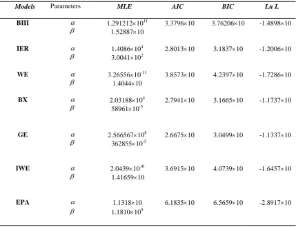
Now, we first estimated the unknown parameters of the different statistical models. For estimation of parameters, maximum likelihood estimation (MLE) was used because it has been considered as the most effective method. Now for comparing spreading data with the proposed distribution functions, we required some measure of the goodness of fit between the functions and data. The Akaike information criterion (AIC), Bayesian information criterion (BIC), maximum likelihood criterion (ln L) and Kolmogorov-Smirnov (K-S) distance are considered as the well-established model selection criteria. The estimated parameter values, AIC, BIC and ln L are reported in Table 1. Also, the Kolmogorov-Smirnov (K-S) distances and the corresponding p -values are presented in Table 2. From Tables 1 and 2, it is observed that
GE BX IER BIII IWE WE EPA
AIC AIC AIC AIC AIC AIC AIC
GE BX IER BIII IWE WE EPA
BIC BIC BIC BIC BIC BIC BIC
lnLGElnLBX lnLIERlnLBIIIlnLIWElnLWElnLEPA
and
GE BX IER BIII IWE WE EPA
KS K S K S K S K S K S K S
It is clear that the EPA distribution has the maximum AIC, BIC, K-S distance and it has the minimum likelihood criterion. Also, the p-value of the EPA is less than significance level (0.05). So, the EPA distribution is the worst fitted model among different models considered here. In addition, other distributions specially BX and GE can be used for modeling the spreading data. But, we want to select the model which is more economical as compared to other alternative models. For comparing of these distributions, we provide the TTT plot which is a convenient tool for examining the nature of the hazard rate and accordingly checking for the adequacy of a model to represent the failure behavior of the data. The TTT plot is presented in Figure 3. For the hazard function of the GE distribution, we have
If 1 the hazard function of GE is increasing.
For1, it has a decreasing hazard function.
Similarly for BX distribution, if 1
2
,
the hazard function of BX is bathtub type and for 1
2
, it has an increasing hazard
function. Therefore from Figure 3, it is clear that the empirical hazard function is increasing. Also in this data, the GE (
=2.566567×10⁸) and BX (
Table 1.Estimatedparameters, AIC, BIC and log-likelihood values for different distributions. Models Parameters MLE AIC BIC Ln L
BIII
1.29121210
11
1.5288710
3.379610 3.7620610 -1.489810
IER
1.408610
4
3.0041102
2.801310 3.183710 -1.200610
WE
3.2655610
-11
1.404410
3.857310 4.239710 -1.728610
BX
2.0318810
4
5896110-5
2.794110 3.166510 -1.173710
GE
2.56656710
8
36285510-5
2.667510 3.049910 -1.133710
IWE
2.043910
10
1.4165910
3.691510 4.073910 -1.645710
EPA 1.131810 6.183510 6.565910 -2.891710
1.1810109
Table 2.The K-S distances and the corresponding p-values.
Method BIII IER WE BX GE IWE EPA
K-S 0.1416 0.1164 0.1713 0.0812 0.0715 0.1692 0.2651
p-Value 0.2688 0.5076 0.1064 0. 8967 0. 9601 0.1143 0.0018
Table 3.Observed and expected frequencies and chi-squared statistics for GE.
Intervals Oi Ei
2
( i i)
i
O E E
2
0.00 – 5.10 5 4.72948 0.015473
1.74634
5.10 – 5.26 8 8.63239 0.046320
5.26 – 5.42 10 10.5311 0.026782
5.42 – 5.58 11 9.18289 0.35956
5.58-5.74 4 6.60193 1.02546
Figure 3. The scaled TTT transformfor spreading data of inclined nano and micro droplets impact.
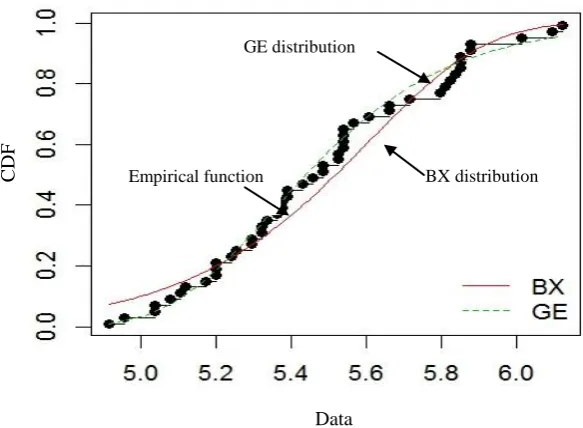
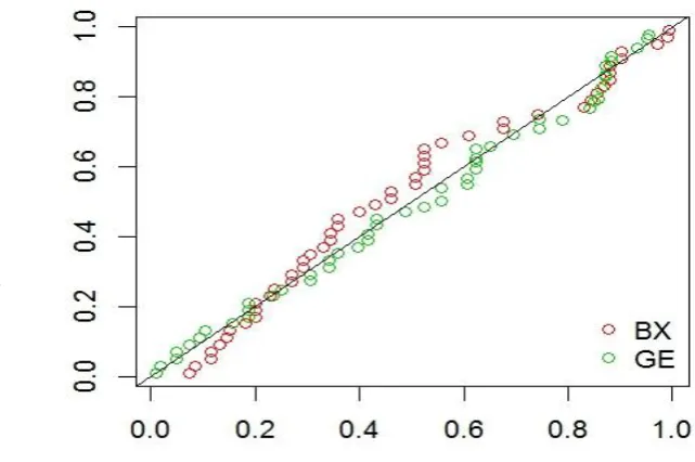
Figure 4. Empirical survival function and the fitted survival functions. Also, it is clear from the Figure 5 that the
data do not deviate dramatically from the line for both the distribution. However, the BX can be used for modeling the data, but a close look at the Figure 5 (also Figure 4) indicates that the graph of GE distribution is closer to the 45-degree line than the graph of BX distribution. So, based on these several criteria and graphical method,
the GE appears to be more appropriate statistical distribution. We also present the chi-square value along with their observed and expected frequencies in Table 3. To calculate the chi-square value, we divided the cumulative distribution function into 6 intervals: [0, 5.10], (5.10, 5.26], (5.26, 5.42], (5.42, 5.58], (5.58, 5.74] and (5.74,∞).
Data
C
DF
BX distribution GE distribution
Empirical function
i/n
φ
(
i/n
Figure 5. The P-P plotfor spreading data of inclined ultrafine droplets impact. The chi-square value is 1.74634, which it
does not lie in the critical regions
2
3, 6.251 (7.815)
at 0.10 (0.05)
signification levels. Therefore, based on the different criteria, test and graphical method, we can say that the GE fits very well to the spreading data more than any other distribution.
5. CONCLUSIONS
In this paper, we had critically analyzed the spreading data of inclined nano and micro droplets impact, using the large class of statistical distributions. We had estimated the unknown parameters using the maximum likelihood method and then had applied five model selection criteria
and test, namely, the minimum AIC and BIC, the minimum Kolmogorov-Smirnov distance, maximum log-likelihood value, and chi-squared test. It was observed that the GE distribution had comparatively more appropriate statistical distribution function for the spreading data. We also had presented different graphical methods such as TTT transform, P-P plot and the empirical survival function and the fitted survival functions. The results showed the efficacy of the GE distribution as a practical alternative to other popular probability models for analyzing the spreading data of inclined impact.
REFERENCES
1. Asadi S., Passandideh-Fard M., Moghiman M., (2008). “Numerical and analytical model of the inclined impact of a droplet on a solid surface in a thermal spray coating process”, Iran. J. Surf. Eng.,4: 1-14.
2. Ghasemi E., Ghahari M., (2015). “Synthesis of Silica Coated Magnetic Nanoparticles”, Int. J. Nanosci. Nanotechnol., 11: 133-137.
3. Habibi M. H., Khaledi Sardashti M., (2008). “Preparation and proposed mechanism of ZnO Nanostructure Thin Film on Glass with Highest c-axis Orientation”, Int. J. Nanosci. Nanotechnol., 4: 13-16.
4. Kang B., Lee D., (2000). “On the dynamic behavior of a liquid droplet impacting upon an inclined heated surface”, Exp. Fluids.,29: 380-387.
5. Kang C., Ng H., (2006). “Splat morphology and spreading behavior due to oblique impact of droplets onto substrates in plasma spray coating process”, Surf. Coat. Technol.,200: 5462-5477.
6. Asadi, S., Passandideh-Fard, M., (2009). “A computational study on droplet impingement onto a thin liquid film”, Arab. J. Sci. Eng., 34: 505-517.
7. Asadi S., (2012). “Simulation of nanodroplet impact on a solid surface”, Int. J. Nano Dim.,3: 19-26. Theoretical distribution function
E
m
p
ir
ical
d
is
tr
ib
u
tio
n
fu
n
ctio
8. Randive P., Dalal A., Sahu K. C., Biswas G., Mukherjee P. P., (2015). “Wettability effects on contact line dynamics of droplet motion in an inclined channel”, Phys. Rev. E.,91: 053006.
9. Jin Z., Sui D., Yang Z., (2015). “The impact, freezing, and melting processes of a water droplet on an inclined cold surface”, Int. J. Heat Mass Transfer.,90: 439-453.
10. Aboud D. G., Kietzig A.-M., (2015). “Splashing threshold of oblique droplet impacts on surfaces of various wettability”, Langmuir.,31: 10100-10111.
11. LeClear S., LeClear J., Park K.-C., Choi W., (2016). “Drop impact on inclined superhydrophobic surfaces”,
J. Colloid Interf. Sci.,461: 114-121.
12. Gupta R. D., Kundu D., (1999). “Theory & methods: Generalized exponential distributions”, Aust. NZ. J. Stat.,41: 173-188.
13. Pasari S., Dikshit O., (2014). “Three-parameter generalized exponential distribution in earthquake recurrence interval estimation”, Nat. Hazards. 73: 639-656.
14. Panahi H., Asadi S., (2016). “A new model selection test with application to the censored data of carbon nanotubes coating”, The Prog. Color. Colorants. Coatings.,9: 17-28.
15. Gupta R. D., Kundu D., (2007). “Generalized exponential distribution: Existing results and some recent developments”, J. Stat. Plan. Infer.,137: 3537-3547.
16. Burr I. W., (1942). “Cumulative frequency distribution”, Annals. Math. Stat.,13: 215-232.
17. Pandiyan P., Bose G. S. C., Sudarvizhi G., Vinoth R., (2012). “Measuring Expected Time to Recruitment in an Organization through Burr Type X Distribution”, Int. J. Math. Res., 4: 95-100
18. Zhou M., Yang D., Wang Y., Nadarajah S., (2008). “Moments of the scaled Burr type X distribution”, J. Comput. Anal. Appl.,10: 523-525.
19. Panahi H., Asadi S., (2011). “Analysis of theType-II Hybrid Censored Burr Type XII Distribution under Linex Loss Function”, Appl. Math. Sci.,5: 3929-3942.
20. Panahi H., Sayyareh A., (2016). “Estimation and prediction for a unified hybrid-censored Burr Type XII distribution”, J. Stat. Comput. Sim., 86: 55-73.
21. Panahi H., Sayyareh A., (2014). “Parameter estimation and prediction of order statistics for the Burr Type XII distribution with Type II censoring”, J. Appl. Stat.,41: 215-232.
22. Panahi H., Sayyareh A., (2014). “Estimation and prediction for a unified hybrid-censored Burr Type XII distribution”, J. Stat. Comput. Sim.,1-19.
23. AL-Hussaini E., (2010). “On the exponentiated class of distributions”, J. Stat. Theory Appl.,8: 41-63. 24. Cheng Y. F., Sheu S. H., (2015). “Robust Estimation for Weibull Distribution in Partially Accelerated Life
Tests with Early Failures”, Qual. Reliab. Eng. Int..
25. Basu B., Tiwari D., Kundu D., Prasad R., (2009). “Is Weibull distribution the most appropriate statistical strength distribution for brittle materials?”, Ceram. Int.,35: 237-246.
26. Mokhlis N. A., (2005), Reliability of a stress-strength model with Burr type III distributions. Commun. Stat. Theor. Meth.,34: 1643-1657.
27. Moradi N., Sayyareh A., Panahi H., (2014). “Estimation of the Parameters of a Exponentiated Burr Type III Distribution under Type II Censoring”, J. Stat. Sci.,8: 93-109.
28. Akaike, H. (1998). “Information theory and an extension of the maximum likelihood principle”, in Selected Papers of Hirotugu Akaike, Springer. p. 199-213.
29. Schwarz G., (1978). “Estimating the dimension of a model”, Ann. Stat., 6 (2), 461–464.
30. Aarset M. V., (1987). “How to identify a bathtub hazard rate”, IEEE Transactions on Reliability, 36: 106-108.

![Figure 2. SEM examination figures that obtained in Kang and Ng [5]. The angles of impact are (a) 10°, (b) 20°, (c) 30°, (d)](https://thumb-us.123doks.com/thumbv2/123dok_us/1311460.1638761/8.595.317.520.408.531/figure-sem-examination-figures-obtained-kang-angles-impact.webp)