Modelling the dynamic response of emergency shut-down valves following full bore rupture of long pipelines

(1)

MODELLING THE DYNAMIC REPONSE OF

EMERGENCY SHUT-DOWN VALVES

FOLLOWING FULL BORE RUPTURE

OF LONG PIPELINES

A thesis submitted to the University of London for the degree of Doctor

of Philosophy

by

Pratik Saha

Department of Chemical and Biochemical Engineering

University College London

Torrington Place

London WCIE 7 JE

(2)

ProQuest Number: U642028

INFORMATION TO ALL USERS

The quality of this reproduction is dependent upon the quality of the copy submitted. In the unlikely event that the author did not send a complete manuscript and there are missing pages, these will be noted. Also, if material had to be removed,

a note will indicate the deletion.

uest.

ProQuest U642028

This work is protected against unauthorized copying under Title 17, United States Code. Microform Edition © ProQuest LLC.

ProQuest LLC

789 East Eisenhower Parkway P.O. Box 1346

(3)

ABSTRACT

This thesis describes the development o f a numerical simulation based on the

method o f characteristics (MOC) for full bore rupture (FBR) o f long pipelines

containing high pressure hydrocarbons. The Peng-Robinson equation o f state

coupled with the assumption o f thermal equilibrium and homogeneous flow are used

to generate the appropriate vapour/liquid equilibrium data. A variety o f solution

techniques including the use o f a second order MOC in conjunction with a nested

grid system have been developed in order to investigate their effects on computation

run times and accuracy.

The above, together with the use o f a DEC Workstation, has allowed for the first

time, the validation o f a MOC model by comparison with intact end pressure data

logged for 20,000s following FBR of the Piper-Alpha main riser. Excellent

agreement is obtained. Comparison with field data obtained following FBR o f LPG

pipelines also gives good agreement.

The main part o f the thesis describes the application o f the simulation for the study

o f the dynamic response o f ball valves and check valves following hypothetical FBR

o f a long pipeline containing either gas or a two-phase mixture. A variety of

scenarios including the effects of valve proximity to the rupture plane and the delay

in closure on the total amount of inventory released prior to pipeline isolation are

analysed. The accompanying pressure oscillations and surges are also accounted for.

The results are in turn used to recommend guidelines regarding the appropriate

(4)

(5)

ACKNOWLEDGMENTS

A special thank you to Dr. Haroun Mahgerefleh for his invaluable support, constant

encouragement and guidance throughout this work.

Many thanks also to my family for always believing it was possible and for their

constant motivation.

Sincerest thanks to my dear friend Renee Boerefijn without whose help, this work

would not have realised its just conclusion.

Finally, I wish to express my gratitude to all my colleagues for creating the right

atmosphere for informed discussions and providing the wit and humour necessary to

(6)

LIST OF CONTENTS

ABSTRACT... 1

ACKNOWLEDGMENTS... 3

CHAPTER 1: INTRODUCTION... 10

CHAPTER 2: THEORETICAL MODELLING OF PIPELINE RUPTURE 2.1 INTRODUCTION... 16

2.2 REVIEW OF THE MATHEMATICAL APPROACHES AVAILABLE FOR THE DERIVATION OF THE CONSERVATION LAWS... 19

2.3 DERIVATION OF THE CONSERVATION LAWS...24

2.3.1 One-Dimensional Flow Assumption...24

2.3.2 Homogeneous Equilibrium Flow Assumption...26

2.3.3 Minor losses and constant cross-section area o f pipe... 29

2.3.4 Horizontal pipeline with no elevation...29

2.3.5 Negligible fluid structure interaction...29

2.3.6 Conservation of M ass... 32

2.3.7 Conservation of Momentum...35

2.3.8 Conservation of energy... 39

(7)

2.5 THERMODYNAMICS OF VAPOUR/LIQUID MIXTURE AND THE 2-

PHASE FLOW M ODEL...51

2.5.1 Deriving the energy equation for a non-ideal homogeneous fluid... 52

2.5.2 The Peng-Robinson Equation o f S tate... 55

2.5.3 Closure relations for the HEM m odel... 56

2.5.3.1 Calculation for a single phase... 57

2.5.3.2 Two Phase F low ... 68

2.6 CONCLUDING REMARKS... 73

CHAPTER 3: NUMERICAL METHODS FOR THE SOLUTION OF HYPERBOLIC SYSTEMS OF EQUATIONS 3.1 INTRODUCTION...74

3.2 HYPERBOLIC EQUATIONS... 76

3.3 FINITE DIFFERENCE THEORY...81

3.3.1 Explicit M ethods... 81

3.3.2 Convergence and global order o f accuracy...84

3.3.3 Consistency and the local truncation error...85

3.3.4 Stabihty... 85

3.3.5 The CFL Condition...86

3.3.6 One-step and multi-step methods...89

3.3.7 Stif& ess...90

3.3.8 Imphcit M ethods...92

3.4 FINITE VOLUME M ETHODS... 95

(8)

3.5 FINITE ELEMENT METHOD...101

3.6 METHOD OF LINES... 104

3.7 METHOD OF CHARACTERISTICS... 106

3.8 REVIEW OF LITERATURE ON PIPELINE RUPTURE... 110

3.9 CONCLUDING REMARKS...121

CHAPTER 4: APPLICATION OF THE MOC FOR FBR SIMULATION AND MODELLING OF ESDV OR SSIV RESPONSE: IDEAL GAS 4.1 INTRODUCTION...122

4.2 CHARACTERISTIC AND COMPATIBILITY EQUATIONS... 124

4.3 FINITE DIFFERENCE APPROXIMATIONS FOR A METHOD OF CHARACTERISTICS SOLUTION... 131

4.4 THE METHOD OF SPECIFIED TIME INTERVALS...135

4.4.1 The First Order Solution...135

4.4.1.1 The Interior Point Calculation... 137

4.4.1.2 The Intact End Point Calculation ...146

4.4.1.3 The Ruptured End Point Calculation... 147

4.4.2 The Second Order Solution...150

4.4.2.1 Interior Point Solution...150

4.4.2.2 Ruptured End Point Solution... 154

4.5 THE INITIAL CONDITION...156

(9)

4.5.3 Summary o f Calculation Procedure...164

4.6 OPTIMISATION AND VALIDATION OF THE FBR IDEAL GAS M ODEL... 165

4.6.1 The modelling o f the fast transient near the ruptured end: Nested grid system...166

4.6.2 The effect o f curved characteristics...174

4.6.3 Intact End Pressures... 175

4.6.4 Heat Transfer Effects... 178

4.7 VALVE CLOSURE MODELLING... 182

4.7.1 Check V alve... 184

4.7.2 Ball Valve... 186

4.8 CASE STUDY... 195

4.8.1 Fluid Dynamics D ata... 195

4.8.2 Mass release data...197

4.8.3 Pressure/time history... 199

4.8.3.1 The effect o f time delay... 199

4.8.3.2 Pressure surge d a ta ...205

(10)

CHAPTER 5: DEVELOPMENT AND VALIDATION OF THE CNGS-HEM

MODEL AND ITS APPLICATION IN PREDICTING ESDV

OR SSIV RESPONSE

5.1 INTRODUCTION... 211

5.2 CHARACTERISTIC AND COMPATIBILITY EQUATIONS... 212

5.3 FRICTIONAL FORCE EFFECTS...214

5.3.1 Unsteady Wall Friction... 215

5.2.2 Steady Flow Friction Factor...219

5.2.3 Flow Dependent Friction Factor...220

5.3.4 Friction factor for two-phase homogeneous flow... 222

5.4 WALL HEAT TRANSFER... 225

5.5 THE INITIAL CONDITION... 226

5.5.1 Steady State Flow ...226

5.5.2 Rupture Plane Calculation at t=0...227

5.6 CALCULATION PROCEDURE FOR CNGS-HEM... 230

5.6.1 Interior point calculation... 230

5.6.2 Rupture Plane Calculation at t>0...231

5.6.3 Calculation at the boundary between grids o f different size... 234

5.7 REVIEW OF RELEVANT EXPERIMENTAL DATA FOR TWO PHASE FBR SIMULATION... 239

5.8 OPTIMISATION OF CNGS-HEM...242

5.8.1 Convergence and accuracy o f first and second order solutions...242

(11)

5.9.1 Rupture o f Piper to MCP-01 subsea line... 257

5.9.2 FBR experiments using LPG at the Isle o f Grain...259

5.10 CASE STUDY - ESDV/SSIV SHUTDOWN PIPER-ALPHA...284

5.10.1 Fluid dynamics data...284

5.10.2 Mass release data...289

5.10.3 Pressure/Time history...291

5.10.4 Pressure Surge... 296

5.11 CONCLUDING REMARKS... 303

CHAPTER 6: CONCLUSIONS AND SUGGESTIONS FOR FUTURE WORK 6.1 CONCLUSIONS... 306

6.2 SUGGESTIONS FOR FUTURE WORK...312

(12)

Chapter 1 Introduction

CHAPTER 1 : INTRODUCTION

Long pipelines are frequently used for the transport o f large quantities of

hydrocarbons under high pressure. In the case o f a typical offshore platform in the

North Sea for example, the amount o f gas present in a 150 km pipeline at 100 bar is

637,000 kg. This represents an enormous source o f energy release which in the event

o f full bore pipeline rupture (FBR) poses the risks o f general and extreme fire

exposure to all personnel in ‘open platform’ areas, and also undermines platform

integrity. The Piper Alpha tragedy (Cullen, 1990) clearly demonstrated the

catastrophic nature of this type o f accident.

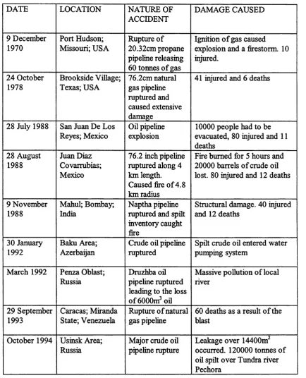
The risk o f FBR is o f course not confined to offshore installations. Table 4.1.1 lists

some o f the documented cases (Bond, 1996) o f pipeline rupture in the past two

decades which have resulted in numerous fatalities and damage to the environment.

In order to isolate and thereby limit the amount o f inventory which may be released

as a result o f pipeline rupture, it is now a statutory requirement (HMSO, 1989) that

for offshore marine pipelines, riser ESDV’s have to be provided. They are always

driven thus excluding certain types o f valve such as check valves which are non

automatic. In addition to riser ESDV’s, protection can also be provided by subsea

isolation valves (SSIV’s) although this is as yet, free o f any statutory requirement.

SSIV’s can be either automatic or non-automatic.

In offshore operations, the responsibility is then placed upon the operators o f the

platform to demonstrate, through the Safety Case (HMSO, 1992), that all hazards

arising from pipeline rupture are addressed and satisfactorily accommodated. Central

to this type o f analysis is the evaluation o f the release rate and its variation with time

in the event o f FBR during isolated (ESDV operating) and un-isolated (ESDV

disabled) release. Such data have an important bearing on almost every safety aspect

(13)

DATE LOCATION NATURE OF

ACCIDENT DAMAGE CAUSED 9 December 1970 Port Hudson; Missouri; USA Rupture of 20.32cm propane pipeline releasing 60 tonnes of gas

Ignition o f gas caused explosion and a firestorm. 10 injured. 24 October 1978 Brookside Village; Texas; USA 76.2cm natural gas pipeline ruptured and caused extensive damage

41 injured and 6 deaths

28 July 1988 San Juan De Los Reyes; Mexico

Oil pipeline explosion

10000 people had to be evacuated, 80 injured and 11 deaths 28 August 1988 Juan Diaz Covarrubias; Mexico

76.2 inch pipeline ruptured along 4 km length.

Caused fire of 4.8 km radius

Fire burned for 5 hours and 20000 barrels o f crude oil lost. 80 injured and 12 deaths

9 November 1988

Mahul; Bombay; India

Naptha pipeline ruptured and spilt inventory caught fire

Structural damage. 40 injured and 12 deaths

30 January 1992

Baku Area; Azerbaijan

Crude oil pipeline ruptured

Spilt crude oil entered water pumping system

March 1992 Penza Oblast; Russia

Druzhba oil pipeline ruptured leading to the loss of 6000m^ oil

Massive pollution of local river

29 September 1993

Caracas; Miranda State; Venezuela

Rupture of natural gas pipeline

60 deaths as a result o f the blast

October 1994 Usinsk Area; Russia

Major crude oil pipeline rupture

Leakage over 14400m^ occurred. 120000 tonnes of oil spilt over Tundra river Pechora

(14)

Basically, there are two types o f valves which may be employed for emergency

shutdown. These include ball valves which are self-activating on sensing a drop in

pressure, or check valves which serve the function o f emergency block valve when

the rupture flow is the reverse o f the normal direction o f flow. Associated with each

valve, there are two characteristic time domains which govern their performance. The

first, here defined as the activation time t„ is dictated by the time lapsed for fluid

disturbances initiated as a result o f FBR to be transmitted from the rupture plane to

the location o f the ESDV. The other, defined as the closure time, t,. is a design

parameter and corresponds to the time it takes for the valve to close from the moment

it is activated until its complete closure. The valve response time, t^ is the summation

o f the two.

The choice o f the appropriate valve presents design and safety engineers with a

dilemma.

The advantage of a check valve is its low t^, thus minimising the amount o f inventory

loss following FBR. This may however be at a cost o f dangerously high pressure

surges resulting from bringing the high velocity escaping fluid to rest (Wylie and

Streeter, 1978); Thorley, 1989; Perko, 1986; Koetzier et. al., 1986). Although such

problems are normally insignificant in the case o f a ball valve due to its gradual

closure, significant amounts o f inventory may escape during this period. This effect

becomes particularly important near the rupture plane where massive amounts of

inventory are released in a very short space o f time. In addition ball valves,

particularly those suitable for offshore applications are very expensive and normally

duplicated.

This thesis describes the development of a mathematical model based on the Method

o f Characteristics (MOC) for simulating fluid dynamic effects following FBR o f long

pipelines containing high pressure gas or two phase mixtures. A variety o f solution

techniques including the use o f nested grid systems in conjunction with second order

characteristics are employed. Their effects on CPU and accuracy are investigated.

This is then followed by application o f the model in predicting the dynamic response

(15)

The development process for a transient two-phase fluid flow model entails three

main steps. Firstly, the basic equations governing the flow, the thermodynamics, and

the initial and boundary conditions need to be formulated. Secondly, an efficient and

accurate method o f resolving these equations needs to be chosen and implemented.

Finally validation o f the model with experimental data or actual records is necessary.

Chapter 2 deals entirely with the first step. The basic partial differential equations of

flow are derived for unsteady quasi-one-dimensional flow o f fluids through a rigid

constant cross-section area o f pipe. The various assumptions made in their

derivations are explained. The derived partial differential equations pertaining to

conservation o f mass, momentum and energy together with an equation o f state

(EOS) constitute a system of equations that are essentially Euler equations with stiff

source terms due to the fliction term in the momentum equation and the heat transfer

term in the energy equation. The thermodynamic relationships that are needed to deal

effectively with the presence o f a real fluid (single and two phase) are also presented.

The appropriate vapour liquid equilibrium data are obtained using the HTSFLASH

programme developed by Michelsen (1982, 1987) incorporating Peng-Robinson

equation o f state (Peng and Robinson, 1976).

In chapter 3, a mathematical description of the hyperbolic nature o f the Euler

equations is described. This is followed by a review o f all available approaches to the

numerical resolution o f the Euler equations including the method o f characteristics

(MOC) which is the preferred method in this study. This is then followed by a

description o f the methods used by various authors to model fluid dynamic effects

during FBR.

Chapter 4 describes the development o f a methodology based on the MOC for the

solution o f the conservation equations in conjunction with an ideal gas. This

involves:

transformation o f the partial differential equations, derived in Chapter 2, to

particular total differential equations called the compatibility equations,

solution o f the compatibility equations based on a new modification to the

(16)

predictor-Chapter 1 Introduction

corrector technique (Zucrow and Hoffinan, 1976) to enhance accuracy o f the

numerical analysis. This technique utilises first order finite difference

discretisation o f the compatibility equations for the predictor step followed by a

second order discretisation for the corrector step.

Various procedures with the primary objective o f reducing the CPU run times

without compromising accuracy in order to produce an optimised model are also

discussed. These include the application o f a nested grid system (CNGS) as well as

the use o f curved characteristics.

Accuracy o f the simulation is assessed by comparing output data with measurements

taken during the Piper Alpha tragedy, and by making comparisons with results

obtained by the models o f Chen et. al (1992).

Some workers such as Flatt (1985), and Olorunmaiye and Imide (1993) respectively

make the assumption o f adiabatic and isothermal flow following FBR. The

deficiencies o f these approaches with respect to accurate prediction over long

depressurisation times, and the influence o f fire on the rate o f heat transfer to the

fluid are also highlighted.

The optimised model is then used to simulate the dynamic response o f emergency

shutdown o f both ball and check valves subsequent to FBR. The principal aim is to

demonstrate the importance o f predicting the rapid variations in the fluid dynamics

within the pipeline during FBR and their influence on the appropriate choice of

ESDV. O f particular interest are the evaluations o f lost inventory and resulting

pressure surges as a function o f valve proximity to the rupture plane and its response

time. Pipelines containing gases whose behaviour may be approximated as ideal are

considered here.

In chapter 5, the CNGS coupled with the Homogeneous Equilibrium Model, (CNGS-

HEM) is used to derive the relevant characteristic and compatibility equations for

simulating FBR o f pipelines containing two-phase multi-component hydrocarbon

mixtures.

(17)

^ use o f a flash calculation procedure for accurate prediction o f fluid properties such

as p, a and P at each node, and at each interpolation point during the numerical

discretisation

^ accurate prediction o f the ‘wall’ friction factor as it is shown that this parameter

has an important effect on fluid dynamics

^ the calculation for the initial conditions (t=0) at the broken end

direct use o f the method o f characteristics to calculate fluid conditions at the

boundaries between the coarse and fine grids. Linear interpolation is not deemed

to be sufficiently accurate for this purpose

use o f curved characteristics near the rupture plane

use o f smaller than maximum permissible At, according to the CFL condition, for

accurate simulation o f the choking condition, thus avoiding numerical instability.

The above is followed by optimisation and validation o f the model by comparison

with various field data. The modifications to the classical ST method and access to a

DEC workstation has meant that the MOC, as used in CNGS-HEM, has been used

for the first time to validate two-phase transient flow in long pipelines over a long

duration (> 30 minutes). Validations o f the CNGS-HEM model are performed in

conjunction with measured data taken after the accidental rupture o f Piper-Alpha, and

also with data regarding the Isle o f Grain pipeline depressurisation tests conducted by

Shell and BP.

The validated model is then used to predict the dynamic response o f ESDV’s or

SSrV’s following FBR o f a pipeline containing a condensable gas mixture and

comparisons are made in terms o f the general trends observed in chapter 4 for

pipelines containing permanent gases.

(18)

Chapter 2 Theoretical Modelling o f Pipeline Rupture

CHAPTER 2: THEORETICAL MODELLING OF

PIPELINE RUPTURE

2.1 INTRODUCTION

Full-bore rupture (FBR) of a high pressure pipeline can be described by a massive

release at the rupture plane followed immediately by a large drop in pressure and

highly transient flow within the pipeline. The development of a transient two-phase

fluid model entails three main steps. Firstly, the basic equations governing the flow,

the thermodynamics, and the initial and boundary conditions need to be formulated.

Secondly, an efficient and accurate method of resolving these equations needs to be

chosen and implemented. Finally validation of the model with experimental data is

needed.

This chapter deals entirely with the first step. The numerical discretisation techniques

available to solve these equations will then be reviewed in Chapter 3 followed by a

review of methods used by past researchers to solve this problem.

Many models exist for the analysis of fluid transients in closed conduit circuits but

only a few are applicable to FBR scenarios. A considerable difficulty has existed in

modelling the fast transient behaviour of the fluid that occurs at the ruptured end,

specifically the choking or critical flow condition that inevitably follows rupture of a

high pressure pipeline. The physical choking condition for a gas states that the flow

velocity equals the local speed of sound which imposes a stiff boundary condition

(Picard & Bishnoi, 1989, Chen, J.R. 1993, Flatt, 1986). This condition is very rare

for liquid flows since the speed of sound for liquids is usually more than 1500 m/s.

For gas flows however, comparatively low local sound speeds (usually about 400

m/s) mean that the choking condition is quickly reached.

The unsteady flow of compressible fluids in pipelines is described by a set of three

(19)

of thermodynamics (energy equation). The fluid properties can be described by an

appropriate equation of state. These together with appropriate auxiliary conditions,

determine the mathematical state of the fluid. The most complete formulation to

describe any fluid flow situation are the Navier-Stokes equations which allow for

variation of fluid property in four dimensions, i.e. the three dimensions of space, x,y,

and z, and also time, t. In order to resolve these equations numerically closure

relations need to be provided to account for both the diffusive and source terms, thus

yielding a system of equations that is extremely complicated.

Solving the full system is the ultimate goal of a numerical flow simulation but the

numerical discretisation necessary to accomplish this for a whole range of fluid flows

is extremely difficult and requires substantial computer resources. In fact, only very

simplified flow systems are computed at present to such a high level of

approximation. It is always necessary to ask the question if it is necessary to resolve

every term in the Navier-Stokes equation. Depending on the type of flow scenario

that needs resolving, certain terms in the equations will have a negligible outcome on

the final solution anyway and can therefore effectively be ignored without any serious

loss of accuracy.

The final form of these equations, ready for numerical discretisation, can be arrived

at through many assumptions and simplifications. Based on the above, the equations

may, in the more general classification, be linear, quasi-linear or non-linear, parabolic

or hyperbolic, and first- or second-order.

Great simplifications to the governing equations can greatly reduce computer run

times, but this might well be at a cost to accuracy of the final solution. For example.

Bell (1978) used a simple exponential model that approximated the mass flowrate by

the sum of two exponentials. This however took no account of either the highly non

linear nature of the discharge, or the type of flow or the length of the pipeline which

has important frictional effects on the flow. The nature of FBR modelling, especially

for two-phase flows when thermodynamic computations such as vapour liquid

(20)

In most o f the studies reviewed, researchers have made various assumptions and

simplifications, in order to suit a particular method of solution or application. Suwan

and Anderson (1992) argued that alternative formulations, interpolations, friction

force representation, or time integration, which may be appropriate for parabolic

problems, will all violate the basic wave like characteristics of a hyperbolic problem.

Most cases o f unsteady one-dimensional flow where disturbance propagation

velocities do not vary significantly, are characterised by quasi-linear hyperbolic

partial differential equations for continuity and momentum. On the other hand,

complex phenomena such as stratified and intermittent stratified-bubble (slug) flows

require a two-dimensional transient analysis for a complete treatment o f the problem.

Various analytical techniques have been used to reduce the number o f equations

before employing the relevant numerical procedure. Van Deen and Reintsema

(1983), for example, introduced a technique which reduces the energy equation to a

single parameter-in-mass equation without the assumption of isothermal or isentropic

flow.

There has been much research activity in many publications in the field o f theoretical

modelling o f fluid transients. Much o f this literature is reviewed in this study.

Following this review, a new methodology based on an approach first proposed by

Picard and Bishnoi (1989) is implemented.

The basic partial differential equations o f flow are derived for unsteady

quasi-one-dimensional flow o f fluids through a rigid constant cross-section area o f

pipe. The various assumptions made in their derivation is explained.

Any two-phase flow model needs accurate vapour liquid equilibrium predictions for

the multi-component fluids and in this study, this is done using the HTSFLASH

programme first developed by Michelsen (1982, 1987). The Peng-Robinson equation

of state (Peng and Robinson, 1976) is used to perform the flash calculations.

Numerical solution o f the basic equations is effected using the method of

(21)

Chapter 2 Theoretical M odelling o f Pipeline Rupture

2.2 REV IEW OF THE M ATHEM ATICAL APPROACHES AVAILABLE FOR

TH E DERIVATION OF TH E CONSERVATION LAWS

A review of mathematical techniques used to date to derive fluid flow equations is

presented in this section. There are three basic methods by which fluid flow problems

are formulated namely, the control volume integral analysis, infinitesimal system

differential analysis, and experimental or dimensional analysis. In all these cases, the

equations of dynamics and thermodynamics must be satisfied.

In the control volume approach, a balance is made between the incoming and

outgoing fluid, and the resultant changes within the control volume and details of the

flow are normally ignored.

In the infinitesimal approach, the conservation laws are written for an infinitesimal

system of fluid in motion and become the basic differential equations of fluid flow.

To apply them to a specific problem it is necessary to integrate these equations

mathematically over the volume, subject to the boundary conditions of the particular

problem. Exact analytical solutions are often possible only for very simple

geometries and boundary conditions, otherwise a numerical solution is needed.

The dimensional analysis approach can be applied to any problem but its inherent

generality makes this type of approach undesirable.

The control-volume analysis is considered the most useful of all the three approaches

as far as practical engineering applications are concerned. It gives results in a

reasonable amount of time with accuracy depending on the assumptions made in

setting up the model.

In fluid flow problems the dependent variables i.e. p, p, u etc. are functions of the

independent variables i.e. t and x in the case of one-dimensional flow. In any given

flow situation, the determination by experiment or theory of the fluid properties as a

function of position and time is considered to be the solution to the problem. There

are two distinct fundamental ways of specifying the flow field, namely the eulerian

(22)

In the Eulerian form the independent space variables refer to a co-ordinate system

assumed to be fixed or translating in space and through which the fluid is moving.

The flow is characterised by a time-dependent velocity field which is to be found by

solving the initial value problem.

In Lagrangian form, the independent space variables refer to a co-ordinate system

fixed in the fluid and undergoing all the motion and distortion o f the fluid, so that the

particles o f the fluid are permanently identified by their Lagrangian variables, while

their actual positions in space are among the dependent variables that need to be

solved.

Although the Eulerian and Lagrangian forms are essentially equivalent, the

Lagrangian form gives more information i.e. it tells where each volume o f fluid came

firom initially and has the virtue that conservation o f mass is automatic. This results

in considerably greater accuracy in some problems.

Ritchmyer (1967) stated that for the above reasons, the Lagrangian form is generally

preferred for some problems in a one space variable. For problems in two or more

space variables and time, the Lagrangian method encounters serious difficulties. In

particular, the accuracy usually decreases seriously as time goes on, due to

distortions, unless a new Lagrangian point-net is defined firom time to time, which

requires cumbersome and usually rather inaccurate interpolations. From this point of

view, the Eulerian form is more attractive. However, the Eulerian form is less adept

at handling interfaces between fluids having different thermodynamic properties

because it provides no simple mechanism to distinguish which kind of fluid is

existent at a given space-time grid point (for problems in one space variable, such a

mechanism can easily be provided). Many schemes have been tried, some combining

the features o f the Lagrangian and Eulerian forms but there is no satisfactory

universal method that has been found for general multi-dimensional problems.

Fashbaugh and Widawsky (1972) stated that the Eulerian formulation is usually used

in steady-state fluid flow problems and the Lagrangian formulation is used more

(23)

information, facilitates easy location o f temperature contact surface propagation

within the pipe. The study by Fashbaugh and Widawsky (1972) compared two

methods, namely the pseudo-viscosity and the Lax-Wendroff numerical method in

modelling the effects o f duct area change on shock strength in one-dimensional

viscous air flow. It was concluded that a one-dimensional variable area Lagrange

analysis is adequate for predicting shock flow through a duct area increase ratio o f at

least 10 to 1.

Ames(1977) stated that until the early 1960’s, the only known stable difference

approximations for the Eulerian form were less accurate than those for the

Lagrangian form. Consequently, the Lagrangian forms are preferred. Both systems

have approximately the same complexity. The major disadvantage o f the Eulerian

system arises when interfaces (shocks) occur separating fluids o f different density.

The Lagrangian form does not have the spatial co-ordinate mesh fixed in advance

and may require refinement o f the mesh as computation advances. This possibility of

re-gridding arises since the Lagrange form is constructed so that mass between two

successive mesh points is approximately conserved.

White (1988) stated that certain numerical analyses o f sharply bounded fluid flow,

such as the motion o f isolated fluid droplets are very conveniently computed in

Lagrangian co-ordinates.

Other more recent writers, including Batchelor (1992) argued that the Lagrangian

type o f specification is useful in certain special contexts but it leads to rather

cumbersome analysis and in general is at a disadvantage in not giving directly the

spatial gradients o f velocity in the fluid.

In fluid dynamics measurements, the Eulerian method is the most suitable. To

simulate a Lagrangian measurement, the probe would have to move downstream at

the fluid particle speeds. The Eulerian formulation has almost exclusively been used

in all recent studies and literature, even in such cases where according to the above

(24)

In this study, both descriptions are used depending on circumstance, with the

Eulerian concept being denoted by {daJd^ or (5a/ôx), and the Lagrangian concept

being denoted by (Da/Dt). The relationship between the two is given by.

Da 5a 5a ^ ^

In the following section the mathematical model used to simulate the transient flow

in a pipeline following FBR is developed. The equations will be derived from first

principles and any assumptions or simplifications will be fully accounted for.

Conservation laws are time-dependent systems of partial differential equations

(usually non-linear or quasi linear) and have a simple structure when in one space

dimension (variation in the y and z directions are neglected). They take the form,

— v(x, t) + — f ( v(x, t)) = Qs (2.2.2)

where v denotes the generic function that is being computed with some numerical

method and is the source term. Here v(x, t) e R*" is an m-dimensional vector of

conserved quantities, or state variables which will be the mass, momentum and

energy terms. More properly, Vj is the density function for the j ’th state variable, with

X2

the interpretation that Jv j(x ,t)d x is the total quantity o f this state variable in the

interval [Xj, X2] at time t.

00

The fact that these state variables are conserved means that |v j(x ,t)d x should be

—00

constant with respect to t. The functions Vj themselves, representing the spatial

distribution o f the state variables with time t, will generally change as time

progresses. The main assumption underlying equation 2.2.2 is that knowing the value

o f v(x, t) at a given point and time allows determination o f flow or flux o f each state

(25)

To see how the conservation laws arise from physical principles, the equation for

conservation of mass in a one-dimensional fluid flow problem is first derived. The

equations derived henceforth will be the full system of Navier-Stokes equations

which are applicable to any flow. The Euler equations which are a simplified version

of the Navier-Stokes equations are then derived with the relevant justifications

(26)

2.3 DERIVATION OF THE CONSERVATION LAWS

This section deals with the mathematical derivation of the conservation laws of mass,

momentum and energy. The assumptions or simplifications made in the following

derivations of the Navier-Stokes equations are,

one-dimensional flow

homogeneous equilibrium fluid flow

negligible minor losses and constant cross section area of pipe

horizontal pipeline with no vertical elevation

^ negligible fluid structure interaction

2.3.1 One-Dimensional Flow Assumption

A flow can be assumed to be one-dimensional if the rate of change of fluid properties

normal to the streamline direction is negligible compared with the rate of change

along the streamline. This means that over any cross-section of the pipe all the gas

properties may be assumed to be uniform. The assumption of one-dimensional flow

gives satisfactory solutions to many problems where either the cross-section area

changes slowly along the path of the stream of gas, the radius of curvature of the pipe

is large compared with its diameter or the shape of the velocity and temperature

profiles are approximately constant along the pipe. For one-dimensional flow of a

fluid, p, p, u etc. are only functions of t and x. The one-dimensional model enables

simpler derivation of the basic equations of pipeline flow.

In real fluid flow situations, especially in the case of high-pressure natural gas flow in

pipelines, the flow cannot be truly one-dimensional because viscous effects will

produce a velocity profile across the pipe with the local velocity zero at the pipe wall

(27)

Ansari (1972) investigated the influence of including radial flow on the solution of

unsteady pipe flow equations. It was shown that neglecting the radial velocity can

lead to substantial error in the determination of the axial velocity of flow. The effect

of the assumption of negligible radial flow was also investigated in relation to

another assumption which is commonly made, i.e. the gradient of the axial velocity in

the axial direction, in viscous flow, is negligible compared to the gradient in the

radial direction. It was found that for slow transients the latter assumption is valid

while the former is not and vice versa for the case of rapid transients The departure

from the one-dimensional flow assumption will be even more pronounced where

there are bends and fittings in the pipeline. Nevertheless, despite the foregoing, the

one-dimensional approximation in gas transmission systems has been shown to be

very good for steady and slowly varying flows.

When the variations in flow are large and rapid, such as in high pressure gas pipeline

ruptures, larger discrepancies are expected from the one-dimensional approximation.

A more rigorous approach is to apply the integrated equation method used in the

turbulent boundary layer theory.

There are many studies and computer models developed for multi-dimensional flow

analysis. A few computer programmes based on multi-dimensional flow models such

as FLOW-3D are commercially available. However, these models can only be

applied to some special cases with confidence.

Shin (1978) discussed the extension of the one-dimensional method of characteristics

to two space dimensions. The extended method uses the same simplifications and

retains the similar simplicity and efficiency as in the conventional one. The

two-dimensional method is applicable to both the Cartesian and axi-symmetric

systems and includes the conventional method as a special case.

Wylie (1983) presented a similar numerical method for analysis of low-velocity

two-dimensional transient fluid flow problems. The method contains similarities to

the one-dimensional method of characteristics but does not follow the traditional

(28)

Chspter 2 Theoretical M odelling o f Pipeline Rupture

The most up to date and comprehensive study is that by Bendiksen and Moe (1993)

and Bendiksen et. al. (1991), which presented the physical basis of a new type of

multi-dimensional two-fluid model, particularly suited for transient flow problems. A

basic difference between this model and the other models is in the solution

procedure, aiming in particular at improved predictions o f transient problems. The

numerical scheme is based on an extension o f an earlier one-dimensional model and

employs an implicit finite difference scheme.

It follows from the above discussion that the three dimensional solution is the natural

method for the FBR problem being modelled if a two-fluid model is to be employed.

As shown in the above mentioned studies, the extension o f one dimensional models

to two-and three-dimensional models could, in principle, be achieved especially if

caution is made in representation o f the other terms in the equations.

2.3.2 Homogeneous Equilibrium Flow Assumption

Transient flows encountered in pipeline rupture problems are frequently two-phase

flow even if the initial state o f the fluid is single phase. The two phases occur either

from liquid condensation due to low temperatures at the rupture plane which then

propagates through the pipeline or for liquid flows, vapour flashing due to low

pressure. A complicated multi-phase flow situation is therefore likely to be

encountered, especially for a multi-component mixture. Convenient classification

into two types o f flow regimes would be dispersed (particles, bubbles and droplets),

and separated (stratified, annular and elongated bubbles) flows. More complex flow

regimes often occur as combinations o f these, such as stratified and annular flows

with entrainment and slug flow. Flow regimes commonly experienced are stratified

(wavy or smooth), annular dispersed, intermittent (slug) and dispersed bubble flows.

In relatively long pipelines, with possibly large pressure losses, several o f these flow

regimes may exist simultaneously as a result o f changing in situ flow rates and

physical properties o f the fluids.

(29)

purpose codes are available. They include FLUENT and RAMPANT, developed by

Fluent Inc., FL0W -3D developed by Flow Science Inc., and PHOENICS developed

by CHAM consultancy. For separated or stratified flow, there has been several

studies, including those by Oliemans (1987); Stadtke and Holtbecker (1991), Philbin

and Govan (1990), and Bendiksen and Moe (1993).

Oliemans (1987) investigated the accuracy o f two-phase flow trunk line predictions

by a one-dimensional steady model for stratified wavy flow in horizontal and

inclined pipes.

Stadtke and Holtbecker (1991) proposed a two-fluid model, i.e. including slip

velocity between the two phases, for transient fluid flow. The complexity associated

with a two-fluid model is that the characteristic equations that define the flow do not

have a simple analytical form. The characteristics in Stadtke and Holtbecker’s model

is derived based on analytical trials rather than physical modelling.

The effect o f concentration stratification in multi-component two-phase flow as a

result o f slip, and mass transfer between the two phases is taken into account by the

computer programmes, PLAC and OLGA developed by Philbin and Govan (1990)

and Bendiksen and Moe(1993) respectively. However neither incorporte proper

phase behavior during the transient flow process due to inherent limitations in the

numerical methods employed.

In the multi-dimensional Moe-Bendiksen model (OLGA), the general two-fluid

equations have been applied with the assumption o f a single pressure field. The

modelling o f constitutive laws at the interface is not general but focused on separated

or stratified flows. A volume equation is applied for the pressure, enabling a direct

two-step solution procedure.

In analysing pressure transients in bubbly air-water mixtures Padmanabhan et. al.

(1978) used a homogeneous model which consists o f one-dimensional equations o f

conservation o f mass for each o f the phases and conservation o f momentum for the

(30)

Bhallamudi and Chaudhry (1990) developed a third-order accurate explicit fmite-

difference scheme for transient flows in one-dimensional homogeneous gas-liquid

mixtures in pipes. The gas-liquid mixture was treated as a pseudo-liquid.

Chen et. al. (1995) used a two-fluid model (MSM), in which the local instantaneous

conservation equations are formulated for each phase. The hyperbolicity of the

equations is achieved by forcing the flow to be marginally stable. Under this

condition, all information related to the structure of the flow that is not considered to

be non-dissipative, inviscid flow is embedded in an inertial coupling constant. To

obtain correct and real sonic characteristics an expression for the inertial coupling

constant is obtained based on critical flow data. The thermodynamic equilibrium

assumption is used as the closure criterion for interfacial mass and energy transfer.

A gas-liquid mixture may be treated as a pseudo-fluid, if the mixture and its motion

may be treated as homogeneous. In the homogeneous equilibrium model (HEM), the

two phases are assumed to move at the same velocity and are always in

thermodynamic equilibrium. The major advantage of HEM is that it has a relatively

simpler mathematical structure and clearly defined characteristic equations are

assured for all flow situations.

Chen et al. (1993, 1995) showed that for long pipelines (length > 100m) the HEM

gave very good agreement with data obtained for fiill-bore rupture from tests

performed by British Gas on the Isle of Grain. The predicted release rate of HEM and

the more detailed two-fluid model, MSM, were very close. It was concluded from

this work that thermodynamic non-equilibrium is insignificant in long pipes except

for the early stages of rarefaction wave propagation.

In the light of the above findings, it is decided to use the HEM assumption in this

work. This means that the following derivations will not contain two separate

momentum conservation equations for each phase of a two-phase mixture and

(31)

2.3.3 Minor losses and constant cross-section area of pipe

Since the aim of this study is the rupture modelling of long, straight pipelines, minor

losses due to bends and obstacles will be neglected in the derivation of the

conservation equations of fluid flow. This assumption is reasonable since these losses

are likely to be small compared with the distributed frictional losses in long

pipelines. The effect of these minor losses on the fluid transients is investigated by

Otwell et. al. (1985).

As regards the assumption of constant cross-section area of pipe, most workers have

generally assumed that the cross-section area of the pipe is not a function of the axial

distance or varies slowly (Flatt, 1985, 1986; Picard and Bishnoi, 1988,1989; Chen,

1993). hi some special cases such as in cooling ducts etc. where the cross-section

area varies appreciably with distance, this effect has been incorporated into the basic

equations. However, in some studies on compressible flow, including those by Zielke

(1968) and Flatt (1989), the equations are based on a variable change in cross-section

area.

2.3.4 Horizontal pipeline with no elevation

The pipeline is assumed to be straight with no elevated sections, therefore the gravity

term is neglected in the equations.

2.3.5 Negligible fluid structure interaction

The classical water-hammer theory only predicts the extreme loading on a system as

long as it is rigidly anchored. When a piping system has certain degrees of freedom

severe deviation from the classical theory may occur due to motion of the system.

Pressure waves exert forces which cause a compliant system to move. As a result of

the motion, pressure waves are formed, a phenomenon known as fluid structure

interaction.

Fluid structure interaction is essentially a dynamic phenomenon, the interaction being

(32)

a piping system are classified in two groups namely distributed forces and local

forces. Typical examples of distributed forces are fluid pressure and friction. In the

case of fluid pressure, rapid pressure fluctuations cause a pipe to expand or contract

thereby creating axial stress waves in the pipe wall. The stress waves in return

generate pressure fluctuations in the enclosed fluid, resulting in a coupling known as

Poisson coupling.

Similarly, friction force is responsible for friction coupling. In most practical

systems, frictional coupling is weak. Local forces act on specific points in a system,

such as elbows, tees or valves and cause axial and lateral motions which generate

pressure waves in the fluid resulting in an interaction called junction coupling.

Junction coupling is generally dominant compared with Poisson and Friction

couplings. Lawooij and Tijsselling (1990) conducted a study of fluid structure

interaction in compliant piping systems. They concluded that the most significant

coupling mechanisms are Poisson and Junction coupling. A simple guideline which

states when interaction is important is formulated in terms of three time scales i.e.,

the time in which the pressure is built up, the eigen-periods of the structure and the

time scale of the water-hammer waves. They also concluded that Poisson coupling is

important for the fluid when significant modes of interaction are dominated by

stiffness.

To consider the motion of the pipe, three main displacements are distinguished

namely axial displacement, lateral displacement and rotation. Therefore in general,

the dynamics of a pipe system are influenced by four wave families, i.e. axial,

flexural and torsional waves in the pipe wall and pressure waves in the fluid. These

co-exist during transience and have different degrees of influence on the transient

behaviour. Fluid structure interaction in compliant piping systems is modelled by

extended water-hammer theory for the fluid and by beam theory for the pipes. In

buried pipelines, the lateral restraint is usually sufficient to ensure that the overall

behaviour is dominated by axial effects. Hence most analyses of fluid structure

(33)

In a study on fluid structure interaction in flexible curved pipes, Stittgen and Zielke

(1990) concluded that the influence of structural motion on the internal pressure is

smaller than the time dependent internal pressure but can still be of influence in

particular cases. They also concluded that pressure waves in flexible pipes are quite

dependent on visco-elastic wall properties.

Rachid and Stuchenbruck (1990) stated that the mechanical properties of the

material, the temperature and the degree of stiffness of the supports, have a

significant influence on the response of the system. Stiffer pipe materials i.e. those

with mechanical damping will experience higher pressures than more compliant pipe

systems. They also found that Poisson effects can induce significant piping motion

especially in long pipe reaches and cause high frequency peaks for pressure and stress

in visco-elastic pipes, e.g. up to 25% above the rigid pipe model. However,

mechanical damping of the pipe material tends to degrade the solid wave front quite

quickly. In most cases, high frequencies generated by the fluid structure interaction

mechanism are virtually eliminated before the first fluid cycle.

In practice the value of the sonic velocity in the fluid in a pipe is influenced by the

elasticity of the confining walls and the compressibility of the fluid. As the elasticity

of the wall materials increases, the effective value of sonic velocity decreases. This

effect is commonly neglected for typical high-pressure gas pipelines. However, some

workers including Wood et. al. (1966), Zielke (1968), Hirose (1971) and Beauchemin

and Marche (1992) have all taken into consideration the effect of pipe elasticity. This

has resulted in an additional term in the continuity equation. In the

Beauchemin-Marche model, no simplification was made on the basic equations and

in addition the effect of variable cross-section area was included.

In the study by Tiley (1989), the effects of fluid structure interaction were not

considered in an effort to maintain simplicity of the model. The same approach is

adopted in this study. It is felt that for long straight pipes that are rigidly anchored as

considered in this work, fluid structure interaction will not be as significant as

(34)

i.e. elasticity of the pipe walls is negligible compared with the compressibility of the

fluid.

2.3.6 Conservation of Mass

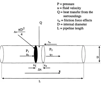
If pipeline rupture occurs at t = 0, then the flow variables can be summarised in

Figure 2.3.1 below:

P = pressure u = fluid velocity

Q = heat transfer from the surroundings

Tw = friction force effects D = internal diameter L = pipeline length 7üD

A=

Uo

Ax

L

Figure 2.3.1: Control Volume

Let X represent the distance along the pipeline and let p ( x , t) be the density of the

fluid at point x and time t. The total mass of fluid per unit cross-sectional area in any

(35)

X2

mass in [x 1, X2 ] at time t = ^ ( x , t)dx (2.3.1)

If we assume that the pipe is impermeable and that mass is neither created nor

destroyed, then the mass in this one section can change only because o f fluid flowing

across the end points x, or X2.

Let u(x, t) be the velocity o f the fluid at the point x at time t. Then the rate o f flow, or

flux o f fluid past this point is given by,

mass flux at (x, t) = p(x,t)u(x,t) (2.3.2)

Therefore the rate o f change o f the mass state variable across the control volume

given by the spatial domain [Xj, X2] is given by.

X2

^ Jp(x,t)dx = p (x ,,t)u (x ,,t)-p (x2,t)u(x2,t) (2.3.3)

This is one integral form o f the conservation law. Another form is obtained by

integrating this in time from time tj to t2, giving an expression for the mass in [Xj, X2]

at time t2 > t, in terms o f the mass at time tj and the total (integrated) flux at each

boundary during this time period.

%2 %2

J p (x ,t2)dx= Jp(x,ti)dx +

Xj Xi

(2.3.4)

Î2 *2

fp (x ,, t)u (x ,,t)dt -

J

p(x2, t)u(x2, t)dt

To derive the differential form of the conservation law, we assume that p(x, t) and

(36)

p(x,t2) - p { x ,t ,) = J ^ p (x ,t)d t (2.3.5)

and.

X2

p(x2,t)u(x2,t)-p (x i,t)u (x ,,t)= J ^ {p (x ,t)u (x ,t)}d x (2.3.6)

*1

Substituting equations 2.3.6 and 2.3.5 into equation 2.3.4 allows one to write,

\ \ \

5 5 1

— p(x,t) + — (p{x,t)u(x,t))|dxdt = 0 (2.3.7)

t , Xi

Since this must hold for any section [Xj, Xj] and over any time interval [tj, tj], it can

be concluded that in fact the integrand in equation 2.3.7 must be identically zero, i.e.,

| p + -^ (p u ) = 0 (2.3.8)

This is the desired differential form o f the conservation law for the conservation of

mass.

For flows where two phases are present and the homogeneous equilibrium flow

assumption is made, the two phases move at the same velocity and a mass balance

for the overall mixture composition, y, in differential form can be written as,

^ ( y i ) + ^ ( u y i ) = 0 i = l , N - l (2.3.9)

(37)

where the subscript i refers to the i’th component o f an N component mixture, a is

the volume fraction o f the vapour phase, and the subscripts 1 and g refer to the liquid

and gas phase respectively.

Equation 2.3.9 shows that the mixture composition is purely convected by the flow

and depends only on the initial fluid composition profile along the pipeline.

2.3.7 Conservation of Momentum

The derivation for the conservation o f momentum is slightly different to that o f mass.

Momentum is a vector quantity and in order to determine all the terms in the

momentum conservation equations it is necessary to define the sources influencing

the variation o f momentum. It is known from Newton’s laws, that the forces for the

variation o f momentum in a physical system are the forces acting on it (Welty et. al.,

1984). These forces consist o f the external volume forces and the internal forces

ZFj. The latter are dependent on the nature o f the fluid considered, and result from

the assumptions made about the properties of the internal deformations within the

fluid and their relation to the internal stresses.

The internal forces acting on the fluid volume in the pipeline within the spatial

domain [Xj, is given by,

^ V j = A P ( x i,t) - A P ( x2,t) + AT(x2,t) - A x ( x i,t) (2.3.11)

where x denotes the viscous shear stresses within the fluid and is a tensor quantity.

These stresses give rise to fluxes that depend on the spatial gradient of the state

variable. In one dimension only, this can be expressed as.

^ 8u 2 0u

5x 3 5x (2.3.12)

where p is the dynamic viscosity o f the fluid

The external volume forces are the forces that would render the flow non-isentropic.

In the assumption o f isentropic flow, this term can be expected to change only

(38)

flows which would be the real case scenario, this is not true. There is likely to be

some destruction o f momentum within this interval and this loss or sink is denoted as

a source term. The source term in non-isentropic homogeneous equilibrium flows can

be attributed to wall friction only. Other hydrodynamic effects such as interfacial

drag force, mass transfer effect force are not relevant for the homogeneous flow

assumption and are therefore ignored with respect to any additional terms in the

momentum equation.

The external force term is therefore.

I

F e = ^ ^ d x A (2.3.13)

where f^ is the fanning friction coefficient. The modulus o f velocity is introduced to

account for change o f direction o f flows.

The total momentum o f fluid in any given volume o f fluid as in that from Xj to Xj can

be given by the following relation for a constant cross-sectional area conduit,

momentum at time t = A j"p(x,t)u(x,t)dx (2.3.14)

where A is the cross-sectional area o f the pipeline (assumed to be constant).

The rate o f flow o f momentum or momentum flux at a point x at time t can be written

as,

momentum flux at (x,t) = p(x,t)u^(x,t)A (2.3.15)

The rate o f change o f momentum within a control volume bounded by the spatial

domain [Xj, X;] will be the sum o f the net momentum fluxes through the volume plus

any internal and external forces acting on the volume. This can therefore be written

(39)

a t A J p (x ,t)u (x ,t)d x = p (x i,t)u ^ ( x i,t) A - p (x2,t)u ^ (x2,t)A

Xl

+ A P(xi, t) - AP(x2, t) + A t(x2, t)

- A t ( x i , t) + dxA

2 D

(2.3.16)

Dividing all sides by A, another form o f this equation is obtained by integrating

equation 2.3.16 in time from t, to tj in order to get an expression for the momentum

in [XjjXj] at time tj > t^.

X2 X2

p(x, 1 2 )u(x, 1 2 )dx = J p(x, 1 1 )u(x, 1 1 )dx +

Xi Xi

t2

j*{p(x 1, t)u^ (x 1, t) - p(x2, t)u^ (x2, t)|d t +

)

{p(xi,t)-p(x

2

,t)}dt +

] '

h ^2

Jf

^pu|u| 4f, ^ I 2 D ;

dxdt

t] Xi

(40)

The following correlations can also be written for momenttmi,

t2

p(x, t2)u(x, 1 2) - p(x, ti)u(x, ti) = | ^ p ( x , t)u(x, t)dt (2.3.18)

%2

p(x2, t)u^(x2, t) - p(xi, t)u^(x,, t) = j ^ [ p U ^ ( x , t)|dx (2.3.19)

]i

(p (x2, t) - p ( x i, t)) = |- ^ p ( x , t)dx (2.3.20)

%2

f

(x(x2 ,t) - t(x i ,t)) = j — x(x,t)dx (2.3.21)

Substituting the relations 2.3.18 - 2.3.21 into equation 2.3.17 and simplifying, we

obtain.

j j l ô t - - - — ^ 5x

t i X,

p(x, t)u(x, t) + ^ [pu^(x, t) + P - x] + p idxdt = 0 (2.3.22)

where p can be written as,

f

P = - 2 - ^ p u lu | (2.3.23)

(41)

^ (p u ) + '^ (p u ^+P-'t^) = - P (2.3.24)

Equation 2.3.24 is the differential Navier-Stokes form of the momentum equation

and is applicable for all flows in all situations.

2.3.8 Conservation of energy

From thermodynamic analysis of fluid continua it is known that the energy content of

a system is measured by its internal energy per unit mass, e. This internal energy is a

state variable of a system and hence its variation during a thermodynamic

transformation depends only on the final and initial states.

The total energy to be considered in a fluid when deriving the conservation equation

is the sum of its internal and kinetic energy per unit mass. Therefore the total energy

per unit mass can be given by,

u^

E = e + - ^ (2.3.25)

A third term, gz, that takes account of the potential energy gained by different pipe

elevations is ignored because the pipe is assumed to run on the same horizontal axis.

The total energy of the fluid contained in the volume bounded by [xi, Xz] can be

given by.

X2

energy in [x^, X2 ] at time t = ^ p(x, t)E(x, t)Adx (2.3.26)

The first law of thermodynamics states that the sources for the variation of the total

energy are the work of the forces acting on the system plus the heat transmitted to

this system.

Considering the general form of the conservation law for the quantity E, then the rate

(42)

convective energy flux at (x, t) = p(x, t)E(x, t)u(x, t)A (2.3.27)

If we consider the general form o f the conservation law, then apart from the

convective flux o f energy there will also be a diffusive flux associated with the

internal energy o f the fluid,

diffusive energy flux at (x, t) = - k ^ ( x , t)A (2.3.28)

where k is the thermal conductivity o f the fluid and T is the absolute temperature.

With regard to the sources o f energy variations in a fluid system, a distinction has to

be made between the surface and the volume sources. The surface sources are the

result o f the work done on the fluid by the internal shear stresses acting on the

surface o f the volume considering that there are no surface heat sources and can be

written at a point as,

surface sources o f energy at (x, t) = - P(x, t)u(x, t)A + x(x, t)u(x, t)A (2.3.29)

The volume sources are the sum o f the work of the volume forces and any other heat

sources other than conduction. This heat source would include any transfer o f

convective heat from the surroundings. In terms o f the volume o f fluid in [Xj, Xj] the

rate o f heat transfer to the fluid from the surroundings can be given by,

Q h = ^ U h ( T , - X ) A d x (2.3.30)

where is the overall heat transfer coefficient and the subscript oo denotes the

conditions external to the pipeline.

The rate o f change o f total energy in [Xj, Xj] can be given by equating the rate form o f

equation 2.3.26 to the difference in fluxes at Xj and Xj and any source terms as

(43)

Chapter 2 Theoretical Modelling o f Pipeline Rupture

X2

(pE)(x,t)Adx = A {(p E u )(x ,,t)-(p E u X x2,t)}

Xl

(2.3.31)

+ a{(Pu)(xi , t) - ^ X 2 . t)} +

+ a{ (tu)(x2, t) - (tu)(xi , t )}

+ Q h + W h

As in the conservation of momentum equation, another form of the above expression

can be obtained by integrating in time from ti to ti, where t2 > ti,

X2 X2 t2

a J * (pE)(x,t2)dx = A j* (pE)(x,ti)dx + j * A {(p E u )(x i,t)-(p E u )(x2,t)}dt

Xl X]

. | a|

+ t2

J

a { (P u )( x , , t) - P u(x2 , t)}dt

^2 ^2

+ J

a { (tu )(x2 , t) - (tu)(xi , t)}dt +

J

(Qh + Wh )dt

ti ti