A Variational Framework for Spectral Discretization of the Density Matrix in Kohn-Sham Density Functional Theory

(1)

A variational framework for spectral discretization of

the density matrix in Kohn Sham density functional

theory

Thesis by

Xin Wang

In Partial Fulfillment of the Requirements for the Degree of

Doctor of Philosophy

California Institute of Technology Pasadena, California

2015

(2)

ii

c

2015

(3)

iii

(4)

iv

Acknowledgements

Getting a PhD is truly a humbling experience. I wouldn’t have been able to make it this far without the unconditional love from my family, the support from my advisors and all of my friends here at Caltech. In the last five+ years, Caltech has become my second home.

I want to first thank my parents for their unwavering support in my education. My life would look very different today if they hadn’t chosen to sacrifice their comfortable life in China to start a new and difficult life in this foreign country. Mom and dad, I am glad that I didn’t disappoint you.

I have been very blessed to have two of the most knowledgable and supportive advisors at Caltech, Prof. Kaushik Bhattachaya and Prof. Michael Ortiz. From them, I learned what it means to be a scientist who hungers after knowledge; I learned how to persevere when confronted with seemingly unsolvable scientific questions. Thank you for giving me this opportunity to learn from you.

(5)

v

Jonathan Chiang, Brandon Runnels and others. I have learned a great deal from you. I want to thank my collaborator, Prof. Thomas Blesgen for his meticulous contributions on our joint paper. I want to thank the class of 2009 PhD students from the Mechanical and Civil engineering, especially the wonderful ladies of our class, Marcella Gomez, Melissa Tanner, Swetha Veeraraghavan, and Jenny Jiang. Thank you for studying with me through the difficult first year and qualification exams. I want to thank the students and postdocs in Kaushik and Michael’s group: Gal Schmuel, Zubaer Hossain, Mauricio Ponga, Likun Tan, Vinamra Agrawal, Lincoln Colins, Dingyi Sun, Paul Plucinsky, Chun-Jen Hseuh (Ren), Jin Yang, Paul Mazur, Landry Fakoua, Stephanie Heyden, Stephanie Mitchell and Sarah Mitchell, for insightful discussions throughout my PhD. I want to thank Stephanie Heyden and Aubrie Amelang for their friendship and all the delicious baked treats they’ve shared with me during my PhD.

(6)

vi

Nomenclature

αI The nondimensional nucleus mass

kf Th fermi level for momentum wavenumber

Ri The Ith nucleus spatial coordinate

ri The ith electron spatial coordinate

V

The space of antisymmetric functions

DN The space of mixed-state N-electron density operators

H L(Ω)

He The space of anti-symmetric wavefunctions for N electrons

Hn The space of wavefunctions for M nuclei

χOPW

k Orthogonal plane-wave basis

I{}() The indicator function for the set {}

IN The space of orbitals for non-interacting electrons

Kj_N The spatially discretized space of KN

KH_N(φ,u) The vector space of density operators in KN that commutes with the Hamiltonian

(10)

x

KH_N,kj(φ,u)

j The vector space of density operators in KN that commutes with the spatiall dis-cretized Hamiltonian Hj(φ, u) in the span of the k binning basis{stk

q}

k q=1

KN The vector space of self-adjoint, trace-class operator in X that has trace N

U The space of exchange-correlation potentials, L4_(Ω)

Uj The spatially discretized space of U

V W₀1,2(Ω)

Vj The spatially discretized space of V

X The vector space of self-adjoint, trace-class operator on S1 with finite kinetic energy XN The space of one-particle reduced density operators

∆k The volume per k-point

∆λ The spectrum width of the Hamiltonian matrix

e₀({R1,· · · ,RM}) The ground state energy for electrons given nuclei positions at{R1,· · ·,RM}

BO₀ The relaxed ground state energy of molecular system with Born-Oppenheimer ap-proxmation

EKS

0 The ground state energy for the extended Kohn-Sham functional

REKS

0 The ground state energy for the reformulated extended Kohn-Sham functional

0 The ground state energy of molecular system - with relaxation of the electrons and

nuclei

KS₀ ({R1,· · ·,RM}) The Kohn-Sham ground state energy

(11)

xi γ The one-particle reduced density operator

γ(r,r0) The one-particle reduced density operator in spatial coordinates ΓN The N-particle density operator

Γ(N,mixed) The mixed N-particle density operator

~ The reduced Planck’s constant

λc Eigenvalue that correspond to core electrons λv _{Eigenvalue that correspond to valence electrons}

λf The fermi energy of the system

λmax The lower bound of spectrum of Hamiltonian

λmin The upper bound of spectrum of Hamiltonian Knp The Krylov subspace of dimension np

N The space of electron densities that come from anti-symmetric wavefunctions with N electrons

V The space of ground state electron density (V-representable)

V The V-representable density

µ The Lagrange multiplier for total number of electrons constraint µξ,ξ The spectral measure with respect to the vector ξi

φ(r) The electrostatic potential

Φ(r,r0) The electrostatic potential operator

(12)

xii ψ(r) The single electron orbital

ψc(r) Eigenvector that correspond to core electrons ψv₍_r_{) Eigenvector that correspond to valence electrons}

Ψe The manybody wavefunction for the electrons

Ψn The manybody wavefunctions for the nuclei

ρ(r) The electron density

ργ(r) The electron density associated with the one-particle density operator γ

σ(HKS_{) The spectrum of}_HKS _operator

˜

ψv₍_r_{) Smoothed eigenvector that correspond to valence electrons}

˜

Tr The approximated Trace operator

+,− The electron spin: up,down εc The correlation integrand

εx The exchange integrand {s_tk

q}

k

q=1 The family of spectral binning basis {tk

q}kq=1 The collection of binning nodes

AI The nucleus spin coordinate

b(r,{R1,· · · ,RM}) The regularized nuclei charge density

B_xc∗ (ρ) The dual functional for Bxc(ρ)

Bxc(ρ) −Exc(ρ), the negative of the exchange-correlation functional

(13)

xiii

CF Constant for homogeneous electron gas kinetic energy

E_bandj (γ) The spectrally discretized band energy E_bandj (γ) The discretized band energy Tr Hj_{(φ, u)γ}

EEKS_{(γ) The extended Kohn-Sham energy functional}

EREKS_{(γ) The reformulated extended Kohn-Sham energy functional}

Eband,j,kj(γ) The spatially and spectrally discretized band energy

Eband(u, φ, γ) The band energy Tr H(φ, u)γ

Ec(ρ) The correlation energy functional

EH(ρ) Classical electrostatic repulsion energy functional, hartree energy

Exc(γ) The exchange-correlation functional written in terms of density operators γ

Exc(ρ) The exchange-correlation energy functional

Ex(ρ) The exchange energy functional

FLL(ρ) The Levy-Lieb universal functional

FL(ρ) The Lieb universal functional

g(λ) The matrix function for density operator

gfermi(λ) The Fermi-Dirac distribution

H The Hamiltonian Operator

h(ρ) The exchange-correlation integrand HKS _{The Kohn-Sham Hamiltonian operator}

(14)

xiv He The Hamiltonian operator for electrons

Hbox The Hamiltonian operator for N identity non-interacting particles in the box

J(γ) The Coulomb energy for the molecular system written as a function of the density operators γ

J(ρ) The Coulomb energy for the molecular system

L(γ) The Lagrangian functional for the reformulated Kohn-Sham energy functional

L(Rl) The distance cutoff between localized basis centers for density matrix entry to be

negligible

Lj_{(γ) The} _discretized _{Lagrangian functional for the reformulated Kohn-Sham energy}

func-tional

M Number of nuclei in the molecular system

me The mass of an electron mn _{The mass of a nucleus}

N Number of electrons

Nd Size of the Hamiltonian matrix

nH The sparsity of Hamitlonian matrix

np Degree of Chebyshev polynomial approximation

nx, ny, nz The quantum number in x,y,and z direction for particle in the box

P(λ) The resolution of identity for HKS

(15)

xv q The charge of an electron

Rc The cut off radius for pseudopotentials.

Rl The localization region for Chebyshev approximations

S(u, φ) The functional for Columb energy

Sj,kj_{(u, φ) The spatially and spectrally discretized functional for Column energy}

T The kinetic energy of the homogeneous electron gas T(u) The dual functional for exchange-correlation

TTF_{(ρ) The Thomas-Fermi kinetic energy functional}

Tj,kj_{(u) The spatially and spectrally discretized dual functional for exchange-correlation} T0(ρ) Kinetic energy functional for non-interacting electrons

Te The kinetic energy operator for interacting electrons

Te The kinetic energy operator for the electrons

Te(ρ) Kinetic energy functional for interacting electrons

TJ(ρ) The Janak kinetic energy functional

Tk(x) Chebyshev polynomials

Tn The kinetic energy operator for the nuclei

TV The kinetic energy per unit volume for homogeneous electron gas

u(r) The exchange-correlation potential, dual function to electron density ρ(r) U(r,r0) The exchange-correlation potential operator

(16)

xvi

Ue−e The electron-electron repulsion energy operator

Ue−e(ρ) The electrostatic repulsion energy functional for interacting electrons

Un−e The nucleus-electron attraction energy operator

Un−n The nucleus-nucleus repulsion energy operator

Vbox The potential for particles in the box

vext(r) The external potential for the molecular system

vKS(r) The Kohn-Sham potential

vxc(ρ) The exchange-correlation potential

ZI The charge of the Ith nucleus

k The electron momentum wave number for homogeneous electron gas

(17)

xvii

Abstract

Kohn-Sham density functional theory (KSDFT) is currently the main work-horse of quan-tum mechanical calculations in physics, chemistry, and materials science. From a mechanical engineering perspective, we are interested in studying the role of defects in the mechanical properties in materials. In real materials, defects are typically found at very small concen-trations e.g., vacancies occur at parts per million, dislocation density in metals ranges from 1010_m−2 _{to 10}15_m−2_{, and grain sizes vary from nanometers to micrometers in polycrystalline}

(18)

xviii

(19)

xix

Chapter 1 Introduction

It is said that in experiments, we have a partial understanding of the full truth; and in computation, we have a full understanding of the partial truth. Therefore, in order to predict new material properties using computation, it is imperative that we build in as much physics as we can into the computational model, provided that it is still computationally feasible. Kohn-Sham Density functional theory (KSDFT) is precisely the theory for electron structure that strikes a good balance between minimizing empiricism in the model and maximizing computational efficiency.

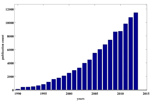
Today, we find DFT in many applications: investigation of phase stability in various materials, oxides, thermoelectrics, ferroelectrics, e.g., Hautier et al. [27], Roy et al. [64], Doak and Wolverton [16], and Bennett et al. Bennett2011, etc; design of new alloys with superior structural properties, e.g., Sandlobes et al. [67], Trinkle et al. [77], and Hickel et al.[31], etc. More recently, DFT has become the primary tool for high throughput screening of materials, e.g., Saal et al. [66], Armiento et al. [4], etc.

(20)

xx

Figure 1.1: Number of publications with DFT as topic.

The development of DFT in 1964 by Walter Kohn was a huge break-through in physics because it linked the ground state energy of the molecular system to the ground state electron density. Kohn transformed the linear eigenvalue problem of finding the ground state of a molecular system from 3N dimensions to a non-linear eigenvalue problem in 3 dimensions, where N is the number of electrons in the systems. There are several good introductions to DFT. The two papers everyone who is interested in DFT should read are the pioneering papers written by Hohenberg and Kohn in 1964 [33] and Kohn and Sham in 1965 [38]. Other helpful introductions to DFT are by Parr and Yang [55], Martin [47], Cances[12], and Anantharaman and Cances [2].

(21)

xxi

For those who are interested in the development of pseudopotentials for density functional theory, the following papers would be useful: the earliest developments of pseudopotentials are found in Hellmann [28], Herring [30], Phillips and Kleinman [61], Antoncik [3]; on norm-conserving pseudopotential Hamann et al. [25], ultrasoft pseudopotential Vanderbilt [79], and separable pseudopotential operators Kleinman and Bylander [37] and Troullier and Martin [78]. Good review articles on pseudopotential can be found in Heine and Cohen [14], Harrison [26], and Pickett [62].

Lastly, for lower complexity algorithms in DFT, such as linear scaling methods, there has been numerous publications since the early 1990s. For density matrix expansion/approximation methods, there are Li et al. [42], Goedecker and Colombo [20], Hernandez et al. [29], Baer and Head-Gordon [6], Suryanarayanaet al.[73], Linet al.[45], Suryanarayana [71], Schofield

(22)

xxii

Chapter 2 Density functional theory

I begin this introduction of DFT from the time-independent Schr¨odinger equation. Almost all of the information in this background section comes from the following two references, the first of which places more emphasis on explanation of the physics [55], and the second of which places more emphasis on mathematics [12].

2.1 Many-body Schr¨

odinger equation

Consider an isolated molecule that consists ofM nuclei andNelectrons. The time-independent Schr¨odinger equation that governs the molecular system without accounting for relativistic effects is,

HΨ =Ψ, (2.1)

where Ψ : _R3(M+N)× {+,−} →_C denotes the wavefunction for the molecular system, and

{+,−} denotes the space of spin degree of freedom; Ψ belongs to the space of He ⊗ Hn,

where

He= N

^

i=1 L2₍

R3× {+,−},C),

and

Hn=L2sds (R 3_×_A

1)× · · · ×(R3 ×AM),C

(23)

xxiii The V

symbol denotes the space of antisymmetric functions due to the fermionic property of the electrons, and the “sds” subscript denotes the system-dependent symmetry properties for the nuclei (even number of nuclei: symmetric; odd number of nuclei:antisymmetric). The spin coordinate of theIth nucleus is denoted byAI, and the electron spins are denoted

by {+,−}. The square of the magnitude of the wavefunction evaluated at a given spatial and spin coordinates {r1,· · · ,rN;R1,· · · ,RM;{+,−}}represents the probability density of

finding the system of nuclei and electrons at{r1,· · · ,rN;R1,· · · ,RM;{+,−}}in 3(M+N)

spatial dimensions. Hence we require the norm of Ψ in He⊗ Hn to be 1; in other words, the

probability of finding all the nuclei and electron is all of space and any spin coordinates is 1.

kΨkHe⊗Hn =

X {+,−} Z R3 · · · Z R3

Ψdr1,· · ·drN, dR1,· · ·dRM = 1. (2.2)

The operator H in equation (2.1) is the Hamiltonian operator of the molecular system:

H = N X i=1 − ~ 2

2me∆ri+

M X I=1 − ~ 2 2mn I

∆RI+

X

1≤i<j≤N

q2 |ri−rj|

+ X

1≤I<J≤M

ZIZJq2

|RI −RJ|

− N X i=1 M X I=1

q2_Z

I

|ri−RI|

,

(2.3) where me_, _mn

I denote the mass of an electron and the Ith nucleus, respectively; q and ZIq

denote the charge of the electron and theIthnucleus;ri andRI denote the spatial coordinate

of the ith electron and theIth nucleus. The Hamiltonian operator is a self-adjoint operator on the space He⊗ Hn.

We can observe the paralell between the quantum Hamiltonian and the classical Hamil-tonian. The following is the kinetic energy operator for the electrons:

Te = N

X

i=1

− ~

2

(24)

xxiv the kinetic energy operator for the nuclei:

Tn= M X I=1 − ~ 2 2mn I

∆RI,

the electrostatic electron-electron repulsion operator:

Ue−e =

X

1≤i<j≤N

q2 |ri−rj|

, (2.5)

the electrostatic nucleus-nucleus repulsion operator:

Un−n=

X

1≤I<J≤M

ZIZJ

|RI−RJ|

,

and the electrostatic nucleus-electron attraction operator:

Un−e =− N X i=1 M X I=1 qZI

|ri−RI|

.

The DFT community commonly uses the atomic units where one sets:

me = 1, q = 1,_~= 1.

Under this system, the electron-nucleus distance in a Hydrogen atom is of order 1, and its ground-state energy is −0.5. The Hamiltonian operator from (2.3) reduces to

H =

N

X

i=1 −1

2∆ri+

M

X

I=1

− 1

2αI

∆RI+

X

1≤i<j≤N

1

|ri−rj|

+ X

1≤I<J≤M

ZIZJ

|RI−RJ|

− N X i=1 M X I=1 ZI

|ri−RI|

,

(2.6) where αI =

mn I

me.

(25)

xxv

to the wavefunction of the molecular system at 0K. In theory, for a system at non-zero temperature, we should take into account eigen-states of the Hamiltonian with higher energy, known as the excited states. For many applications, the calculation of the ground-state is needed for approximation of the excited states.

Finding the ground-state in equation (2.1) corresponds to finding the infimum of the Rayleigh quotient of H:

0 = inf Ψ∈He⊗Hn

hΨ|H|Ψi, (2.7)

where h·|·idenotes the inner product associated with the space He⊗ Hn.

It would take an audacious scientist to attempt to solve for the eigen-states of the time-independent Schr¨odinger equation (2.7). The wavefunction Ψ is a function defined on 3(M+ N) dimension, not counting the spin degree of freedoms. To illustrate the impossibility of solving the Schr¨odinger equation, suppose that one discretizes each spatial dimension into 100 pieces. The system of equations would involve 1003(M+N) _{degrees of freedom, which}

equals 10600 for a system of 50 nuclei and 50 electrons.

(26)

xxvi

2.1.1 Born-Oppenheimer Approximation

The key assumption behind the Born-Oppenheimer approximation is that the motion of the nuclei is slow relative to the motion of the electrons, such that at every movement of the nuclei, the electrons have reached their ground-state configuration. In other words, the characteristic time scale to achieve equilibrium for the nucleus is much longer than the characteristic time scale of equilibrium for the electrons. Hence we can treat the spatial coor-dinates of the nuclei {R1,· · · ,RM}as a parameter, and find the ground-state wavefunction

of the electrons for a given set of nuclei coordinates. This assumption is supported by the observation that the mass of a nucleus is at least 1800 times the mass of an electron.

Mathematically, the Born-Oppenheimer approximation allows us to separate the wave-function Ψ into a singleproduct of an electron wavefunction and a nuclei wavefunction:

{Ψ = ΨeΨn: Ψe ∈ He,kΨekHe = 1,Ψn∈ Hn,kΨnkHn = 1}.

Substitute this approximation into the Rayleigh quotient in equation (2.7), and we get

BO₀ = inf

Ψn∈Hn

{

Z

R3

· · ·

Z

R3

− 1

2αI

|∇RIΨn|

2₊e

0(RI,· · · ,RM)

|Ψn|2)dRI· · ·dRM}, (2.8)

where

e₀(RI,· · · ,RM) = Un−n+ inf

Ψe∈He

hΨe|He|Ψei

hΨe|Ψei

, (2.9)

with the electronic Hamiltonian He defined by

He = N

X

i=1 −1

2∆ri +

X

1≤i<j≤N

1

|ri−rj|

(27)

xxvii where

Vext(r1,· · · ,rN,{R1,· · · ,RM}) = N

X

i=1

vext(ri,{R1,· · · ,RM}) = N

X

i=1

_XM

I=1

ZI

|ri−RI|

. (2.11) We will refer to potential due to the nuclei in the electronic problem (2.9) as an external potential; the potential due to the electrons are internal to the problem. The classification of everything that is not electronic potential to be external potential allows us to consider other applied potentials such as electric or magnetic potential on the electronic system in the same generalization. Note that we have adopted a slight abuse of notation where h·|·i

has been to used to denote both the inner product defined on He and Hn.

In the limit that the mass of the nuclei go to infinity, the kinetic energy of the nu-clei can be neglected, and the wavefunction of the nunu-clei is concentrated on the points

{RI,· · ·RM}, since the deBroglie wavelength of a nucleus is infinitesimal compared to the

deBroglie wavelength of an electron. The infimum problem in equation (2.8) becomes a geometry optimization problem:

BO₀ = inf

{RI,···,RM}⊂R3M

e₀(RI,· · · ,RM).

The solution of the Schr¨odinger equation can be solved in two steps: first solve for the electron ground states, by finding the lowest eigenvalue and its corresponding eigenfunction of the electronic Hamiltonian He; then solve a geometry optimization problem to get the

ground-state energy of the molecular system. The most important consequence of the Born-Oppenheimer approximation is that the electronic Hamiltonian He has a purely discrete

(28)

xxviii

2.2 Precursors to density functional theory

The word “density” in density functional theory refers to the electron number density in three dimensions. It is commonly referred to as the electron density of the system; we denote it by ρ(r). One should not confuse the electron density with the probability density in equation (2.2). We will describe subsequently how to obtain the electron density from the probability density given by the electron wavefunction Ψe(r1,· · · ,rN).

In 1964, Kohn and Hohenberg proved that the electronic ground-state energy of the system in equation (2.9) is a unique functional of the electron density derived from ground-state wavefunction. Looking at the minimization problem in equation (2.9); it is not obvious to see why the electron density is relevant. What led Kohn and Hohenberg to the electron density of the system? In fact, Kohn-Hohenberg did not conjure up the concept of the electron density out of nothing. Prior to DFT, there had been a number of approximate methods developed based on relating the electron density to the ground-state energy; these are the Thomas-Fermi models. The motivations for introducing the Thomas-Fermi model in this thesis are two-fold: firstly, it will serve as a transition from the electron ground-state energy as a functional the many-body electron wavefunction Ψe(r1,· · · ,rN) in (2.9)

to electron ground state as a functional of the electron density; secondly, the exchange energy functional of the local density approximation, which is a key component of density functional, is taken from the same assumptions of the Thomas-Fermi models. Next we will introduce briefly the Thomas-Fermi models. The spin degree of freedom will be neglected in the following discussion for simplicity.

(29)

xxix

as described, and the Hamiltonian of the system inside the box is

HΨe(r1,· · · ,rN) = N

X

i=1

∆riΨe(r1,· · · ,rN) = EΨe(r1,· · · ,rN),

subject to the boundary condition,

Ψe(r1,· · ·,rN) = Ψe(r1 +l,· · · ,rN +l).

Since the Hamiltonian is separable with respect to the spatial coordinate of each electron

ri, the electron wavefunction Ψe can be written as a Slater determinant of single electron

orbitals [69]:

Ψe=

1

√

N!det

        

ψ1(r1) ψ2(r1) · · · ψN(r1)

ψ1(r2) ψ2(r2) · · · ψN(r2)

..

. ... ...

ψ1(rN) ψ2(rN) · · · ψN(rN),

        

(2.12)

where the orbitals {ψn(r)}n∈_Z are the eigenfunction to the single electron Hamiltonian in a

box:

Hboxψn(r) =−

1

2∆rψn(r) =λnψn(r), (2.13) with the periodic boundary condition:

ψn(r) = ψn(r+l).

The Slater determinant form ensures that the wavefunction Ψeis antisymmetric with respect

to exchange of spatial coordinates.

Without considering the boundary conditions, the following solution for the orbitals satisfies the single-electron Hamiltonian in equation (2.13):

(30)

xxx and

λk=

|k|2

2 .

As a result of the boundary conditions, the wavefunction kcannot take arbitrary values; its corresponding wavelength in each spatial dimension has to be an integer multiple of the length of the box. The periodic boundary condition has quantized the wavenumber k. The quantized wave numbers are k ≡ [2πnx

l ,

2πny

l ,

2πnz

l ], x, y, z represent each direction in space,

and n ≡ [nx, ny, nz], and ni = · · ·,−2,−1,0,1,2,· · ·. The corresponding eigenvalues are

also quantized according to the quantization of the wave numbers, but since energy levels are proportional to|k|2_{, there will be degenerate eigen-states, i.e., wavefunctions that differ}

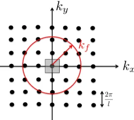
in wavenumber but that have the same energy. The electron levels will be filled according to the Pauli-exclusion principle, with only two electrons (assuming a spin-paired system) occupying a given wavefunction with a wavenumber k. The wavefunctions that correspond to the lowest energy will be occupied first at the ground state. The maximum energy reached by a system of N electrons is called the fermi energy, λf, and the corresponding magnitude

of wavenumber kf =|kf|, the fermi wavenumber. We can find what λf and kf for a given

(31)

xxxi

points within the circle marked by a radius of kf in Figure 2.1 by

Np ≈

πk2

f

∆k.

This approximation improves as the space between grid points decreases. In three

dimen-Figure 2.1: k-points in two dimensional k-space.

sions, we can define fermi wavenumber magnitude by:

kf = N

2∆k 4 3π

1/3

= 3π

2_N

l3

1/3

. (2.14)

At this point, we can define a quantity which is going to be the central quantity in DFT, the electron number density, or simply the electron density:

ρ = N l3.

We can express both the fermi energy and the fermi wavenumber magnitude as a function of electron density ρ:

kf = (3π2ρ)1/3. (2.15)

and

λf =

(3π2_ρ)2/3

(32)

xxxii

And to calculate the total (kinetic) energy of the system, the bruit force method would be

T = 2X

k

λ(k)f(λ), (2.16)

where f(λ) is the occupation function of the energy levels:

f(λ) =

    

1, if λ≤λf,

0, otherwise.

To use the approximation that the box is large, we can write the summation over k in equation (2.16) as an integral in three dimensions,

T = 2X

k

λ(k)f(λ) = 2 ∆k

X

k

λ(k)f(λ)∆k

≈ l

3

4π3

Z

λ(k)f(λ(k))dk. (2.17)

Since we know that the energy is only a function of |k|, we can integrate equation (2.17) using spherical coordinates,

T(kf)≈

l3 4π2

Z kf

0

k4

2 λ(k)dk.

After integration, we can use the relation between kf and electron density ρ in

equa-tion (2.15), and write the total kinetic energy of the system as a funcequa-tion of the electron density:

T ≈ 3

10(3π

2₎2/3_l3_ρ5/3_,

or kinetic energy per unit volume:

TV =

T l3 =

3 10(3π

2₎2/3_ρ5/3 _≡_C

(33)

xxxiii

The system described above is also called a system of homogeneous electron gas since only homogeneous electron density ρ = N_l3 enters into the equation (2.18). The Thomas-Fermi

model approximates the kinetic energy per unit volume of theinhomogeneous electron gas by carving up the system into pieces oflocallyhomogeneous electron gas, as shown in Figure 2.2. The kinetic energy of the system of the inhomogeneous system is

T =

n

X

i=1

CFρ

5/3

i Vi.

In the limit of the homogenous volumes Vi → 0, the summation becomes an integral; we

arrive at the Thomas-Fermi kinetic energy functional, as a function of the electron density:

TTF(ρ) = CF

Z

Ω

ρ(r)5/3dr.

It is important to emphasize that the locally homogeneous approximation of the

inhomo-Figure 2.2: A inhomogeneous electron gas divided into pieces of locally homogeneous electron gas.

geneous electron gas is only appropriate when the electron density varies very gradually in space. For instance, this assumption works well for metallic systems where the electrons are not locally bound to any nucleus, but it works poorly for systems with ionic or covalent bonds since the electrons tend to be bound to a given nucleus.

(34)

xxxiv interaction energy,

U_nTF₋_e=

Z

R3

M

X

i=1

Zi

|Ri−r|

ρ(r)dr,

and

U_eTF₋_e = 1 2

Z

R3

Z

R3

ρ(r)ρ(r0)

|r−r0| drdr

0

.

So we have arrived at the Thomas-Fermi energy functional as a function ofonlythe electron density ρ(r):

E(ρ) =CF

Z

R3

ρ(r)5/3dr+

Z

R3

M

X

i=1

−Zi

|Ri−r|

ρ(r)dr+ 1 2

Z

R3

Z

R3

ρ(r)ρ(r0)

|r−r0| drdr

0

, (2.19)

where CF = ₁₀3 (3π2)2/3.

The Thomas-Fermi ground-state energy can be found by minimizing the energy functional in equation (2.19) with the constraint that the total number of electrons is N:

Z

R3

ρ(r)dr =N.

(35)

xxxv

2.3 Electron density and Hohenberg-Kohn Theorem

Before we state the Hohenberg-Kohn theorem and its proof, we would like to introduce the electron density and its relation to the many-body electron wavefunction Ψe.

2.3.1 Electron density

It is quite easy to get an intuitive understanding of what the electron density means physically from the homogenous electron gas; it is less obvious how to find the electron density beyond the homogenous electron gas.

Let us begin by considering |Ψe(x1,· · · ,xN)|2, the probability density of finding electron

1 at x1, electron 2 at x2,· · ·, electron N at xN, where x≡(r :σ), and σ∈ {+,−}. Then

hΨe|Ψei=

X

σ

Z

R3 · · ·

Z

R3

| {z }

N

|Ψe(r1,· · · ,rN)|2dr1,· · · , drN = 1,

is the total probability of finding electron 1 in all of_R3, electron 2 in all of_R3,· · ·, electron N in all of _R3. Following suit, we can understanding the following quantity, defined by,

PΩ(r1) =

X

σ

Z

Ω

Z

R3

· · ·

Z

R3

| {z }

N−1

|Ψe(r1,r2,· · · ,rN)|2dr1,· · ·,drN, (2.20)

as the total probability of finding electron 1 in volume Ω, and electron 2 in all of _R3 _{· · ·}_,

electron N in all of R3. In other words, independent of the remaining electrons, the proba-bility of finding 1 electron in Ω is PΩ, and I expect to find PΩ fraction of electron 1 in Ω.

Since all the electrons are identical, the total number of electrons we expect to find in Ω is

nΩ =NPΩ(r)

=

Z

Ω

(36)

xxxvi

where ρ(r) is the electron density of the molecular system, using equation (2.20):

ρ(r) =NX

σ

Z

R3

· · ·

Z

R3

| {z }

N−1

|Ψe(r,r2,· · · ,rN)|2dr2,· · · , drN.

From the definition of the electron density, we see that the ground-state wavefunction con-tains more information about the electronic system than the electron density alone. Given a wavefunction, we can always find its corresponding electron density through integration; but given only the electron density, we cannot recover the wavefunction. There may be many wavefunctions that will yield the same electron density.

Next we will state the Hohenberg-Kohn theorem and its proof [33].

2.3.2 Hohenberg-Kohn theorem

Theorem 1 The ground-state electron density in the electronic problem in equation (2.9)

determines uniquely up to a constant the external potentialVext(r1,· · · ,rN)in equation (2.11)

of the system.

Proof The proof in [33] assumes the non-degeneracy (i.e., uniqueness) of the ground-state wavefunction in equation (2.9), and we will reproduce their proof for completeness. We will discuss later how this assumption can be lifted as result of the work by Lieb, et al. [43].

Hohenberg and Kohn proved theorem 1 with proof by contradiction. Suppose for a system of N electrons, there exists two external potentialsVext,1, and Vext,2 defined by

Vext,1(r1,· · · ,rN) = N

X

i=1

vext,1(ri)

and

Vext,2(r1,· · · ,rN) = N

X

i=1

vext,2(ri).

(37)

wave-xxxvii

functions from equation (2.9) that yield the same electron density.1 _{Let us denote the}

Hamiltonians corresponding to the two external potentialsH1 and H2, respectively:

H1 =Te+Ue−e+Vext,1

and

H2 =Te+Ue−e+Vext,2,

whereTeandUe−eare defined in equations (2.4) and (2.5). Their corresponding ground-state

wavefunctions, Ψe,1 and Ψe,2. Notice that H1 and H2 differ only by the external potential.

Now consider the variational problem in equation (2.9); for H1, we have,

E1 =hΨe,1|H1|Ψe,1i= inf Ψe∈He,kΨekHe=1

hΨe|H1|Ψei

<hΨe,2|H1|Ψe,2i=hΨe,2|Te+Ue−e|Ψe,2i+hΨe,2|Vext,1|Ψe,2i;

similarly, consider the variation problem (2.9) for H2:

E2 =hΨe,2|H2|Ψe,2i= inf Ψe∈He,kΨekHe=1

hΨe|H2|Ψei

<hΨe,1|H2|Ψe,1i=hΨe,1|Te+Ue−e|Ψe,1i+hΨe,1|Vext,2|Ψe,1i.

Next we take advantage of the fact that H1 and H2 only differ by the external potential:

=E2+hΨe,2|(Vext,1−Vext,2)Ψe,2i, (2.21) 1_{If the potentials differ only by a constant, then the variational problem (2.9) would yield the same}

(38)

xxxviii and similarly,

=E1+hΨe,1|(Vext,2−Vext,1)Ψe,1i. (2.22)

One can show after some algebra that

hΨe,1|(Vext,2−Vext,1)Ψe,1i=

Z

R3

vext,2(r)−vext,1(r)

ρ(r)dr=−hΨe,2|(Vext,1−Vext,2)Ψe,2i.

Adding equation (2.21) and equation (2.22), we get

E1+E2 < E1+E2.

Therefore, there cannot exist two external potentials by differing more than a constant that has the same ground-state electron density.

From the Hohenberg-Kohn theorem, given a ground-state electron density, we can determine the number of electrons by integration, and the external potential is determined up to a constant, thus the Hamiltonian is completely determined, and consequently the ground-state energy is completely determined. Further from the variational problem (2.9) for an external potential Vext,1,

E1 =hΨe,1|H1|Ψe,1i=hΨe,1|Te+Ue−e|Ψe,1i+

Z

R3

vext,1(r)ρ(r)dr,

there must exist a functional, FHK(ρ), such that,

(39)

xxxix

where Ψe,1 is the ground-state electron wavefunction for Hamiltonian H1. The functional

FHK is a universal functional,i.e., independent of the external potential of the system; it

depends only on the number of electrons in the system N. Hohenberg and Kohn further showed in [33] that there is a variational principle with respect to the electron density for a given external potential:

E0 = inf

ρ∈VEHK(ρ) =FHK(ρ) +

Z

R3

vext(r)ρ(r)dr, (2.23)

where V is the space of electron densities that come from ground-state wavefunctions, also known as aV-representable electron densities. There are still two major open questions that remain in the Hohenberg-Kohn energy functional:

1. The exact form of the universal potential FHK(ρ) is unknown.

2. The necessary and sufficient conditions for the space V is unknown.

These two open questions render the Hohenberg-Kohn energy functional to a theoretical result; nevertheless, it illuminated a very promising direction for quantum mechanical cal-culations.

2.4 Kohn-Sham density functional theory

A year later, in 1965, Kohn and Sham [38] came up with an approximation toFHK using the

Slater determinant form of electron orbitals in equation (2.12), known as the Kohn-Sham density functional theory. Kohn and Sham sought to solve the first of the two open problems, and neglected the second open problem in their formulation. We restrict the discussion to spin-unpolarized systems for simplicity.

(40)

xl

leaving the remaining unknown quantities to modeling:

FHK(ρ) =T0(ρ) +EH(ρ) +Exc(ρ). (2.24)

The first term in equation (2.24) is the kinetic energy of the electrons if they are non-interacting electrons; the second term,

EH(ρ) =

1 2

Z

R3

Z

R3

ρ(r)ρ(r0)

|r−r0| ,

is the electron-electron repulsion energy if the electrons are classical, also known as the Hartree energy of the system.

The last term contains the remaining interaction energy that has not been accounted for, and it is called the exchange-correlation energy of the system. The exchange-correlation energy functionals were first approximated using the exchange and correlation energies of a locally homogeneous electron gas as described in section 2.2. With these approximations, the Kohn-Sham energy functional becomes

EKS(ρ) =T0(ρ) +

Z

R3

Z

R3

ρ(r)ρ(r0)

|r−r0| +Exc(ρ) +

Z

R3

vext(r)ρ(r)dr. (2.25)

Taking the first variation with respect to the electron density of the Kohn-Sham functional in equation (2.25), subjecting to the constant,

Z

R3

ρ(r)dr =N, (2.26)

we arrive at the Euler-Lagrange equation for the Kohn-Sham energy functional:

δT0

δρ +

Z

R3 ρ(r)

|r−r0|dr

0

+δExc

δρ +vext(r) +µ= 0, (2.27)

(41)

xli

Kohn and Sham observed that the Euler-Lagrange equation (2.27) for a non-interacting electron system under the external potential is

vKS(r) = vext(r) +

δExc

δρ +

Z

R3 ρ(r)

|r−r0|. (2.28)

With the assumption that all non-interacting electron systems that are subject to an external potential admit minimizers of the Slate determinant form (2.12), Kohn and Sham came up with an orbital formulation to Hohenberg-Kohn density functional theory. Recall from section 2.2 that the ground-state orbitals of a system of non-interacting electrons can be found by writing the single electron Hamiltonian and selecting its eigenfunctions according to the Pauli-exclusion principle. The corresponding Kohn-Sham single electron Hamiltonian is

HKSψi =

− 1

2∆ +vKS ρ(r)

ψi =λKSi ψi. (2.29)

The corresponding ground-state electron density of the Kohn-Sham system is

ρ(r) = 2

N/2

X

i=1

|ψi(r)|2, (2.30)

where the orbitals ψi are the eigenfunctions that correspond to the first N/2 lowest

eigen-values. Subsequently, the kinetic energy functional takes the form

T0(ρ) = 2

Z

R3

N

X

i=1

|∇ψi(r)|2dr.

We can rewrite the Kohn-Sham energy functional in equation (2.25) as a functional of single electron orbitals:

EKS(ρ) = 2

Z

R3

N/2

X

i=1

|∇ψi(r)|2dr+

Z

R3

Z

R3

ρ(r)ρ(r0)

|r−r0| drdr

0

+Exc(ρ) +

Z

R3

(42)

xlii

subject to the constraint that the orbitals have to be orthonormal:

Z

R3

ψi(r)ψj(r)dr=δij.

Note that the Kohn-Sham single electron Hamiltonian in equation (2.29) is a non-linear functional. The Kohn-Sham potential vKS is a function of the electron density, which is a

function of the eigenfunctions of the Hamiltonian in equation (2.30). The solutions of the eigenvalue problem in equation (2.29) can be carried out self-consistently, by starting with an initial guess of electron density ρ0, and obtaining a Kohn-Sham potential vKS(ρ0), and

finding the corresponding lowest eigenvalues ofHKS(ρ0) and then updating the new electron

density. This procedure is repeated until a self-consistent density is produced.

2.4.1 Exchange-correlation functional

Since KSDFT is formally exact with the exact exchange-correlation function, the approx-imation of the exchange-correlation functional is critical to its accuracy. There has been numerous flavors of exchange-correlation functionals developed since 1965. For more infor-mation on exchange-correlation functionals, one can refer to [55] and [47]. In their semi-nal paper [38] Kohn and Sham proposed the local density approximation(LDA). The LDA exchange-correlation functional is based on the inhomogeneous electron gas model as dis-cussed in section 2.2.

The exchange-correlation energy is split into exchange and correlation contributions:

Exc(ρ) =Ex(ρ) +Ec(ρ) =

Z

R3

ρ(r) εx(ρ) +εc(ρ)

dr.

(43)

xliii

description of the electron density (see section 2.6.1 for a detailed description), defined by:

γ(r,r0) = 2

N/2

X

n=1

ψn(r)ψn∗(r

0

).

The exchange energy from the HF approximation is

Ex(ρ) =

1 4

Z

R3

Z

R3 1

|r−r0|γ(r,r

0

)drdr0. (2.32)

Recall from section 2.2 the nth orbital for the particle in the box is

ψn(r) =

1

V1/2 exp(ir·kn).

The corresponding one-particle density operator is

γ(r,r0) = 2 V

N

X

n=1

exp ikn·(r−r

0

)

. (2.33)

In the limit of the homogenous electron gas (i.e., the limit ofV → ∞and N → ∞such that ρ(r) = N_V is finite) we can replace the summation in equation (2.33) with an integral after multiplying by ∆_∆k_k:

γ(r,r0) = 1 4π3

Z

R3

exp ik·(r−r0). (2.34) Substitute equation (2.34) into the HF exchange energy in equation (2.32), and we simply obtain the exchange energy for the homogeneous electron gas:

Ex(ρ) =Cx

Z

R3

ρ(r)4/3dr, (2.35)

with Cx= 3₄(_π3)1/3. This exchange energy was first calculated by Dirac in [15].

(44)

xliv of rs, defined by:

4 3πr

3

s =

1 ρ.

The different approximations of the correlation functional come from either random phase ap-proximations [81] or numerical calculations of homogenous electron gas in Quantum Monte-Carlo [13]. Since then, more sophisticated exchange-correlation functionals beyond LDA have been introduced in order to increase the accuracy of Kohn-Sham calculations. Some examples include generalized gradient approximation (GGA) [58] and hybrid functionals [8]. We will not go into details on these approximations.

Returning to LDA, the first Kohn-Sham LDA calculations was performed by Tong and Sham in 1966 [76]. Since then, Kohn-Sham density functional theory has become the work-horse of quantum mechanical calculations today.

2.4.2 Pseudopotentials

In the numerical practice of DFT, we often make what is known as the pseudopotential approximation; since it is known that the core electrons in the atom often do not participate in the formation of bonds between atoms, we can assume that the core electron orbitals are “frozen”, and can be transferred from a simpler configuration such as a single atom to more complex molecular environments. The adoption of pseudopotential brings two advantages in computation: first, the number of electron orbitals is reduced to only the number of valence electrons in the system; second, the pseudopotential allows us to remove the rapid oscillation of the valence electrons orbitals near the nucleus, which was caused by the orthogonality constraint to the core electron orbitals, hence allowing fewer number of basis to represent the valence electron orbitals in numerical discretization.

(45)

xlv

near the nucleus. The idea of the pseudopotential approximation pre-dates the development of density functional theory, and has been used in many-body wavefunction formulations as well as independent-electron formulations such as Hartree-Fock methods. The concept that led to psedudopotentials used today was the orthogonal plane wave method by Herring in 1940 [30]. The original idea in Herring was to augment the plane-wave basis functions with some other functions that are centered on the nucleus cores so as to reduce the number of plane-wave basis required to represent the valence states. To avoid ill-condition, Herring removed the projection of the nuclei-centered functions from the plane-wave basis:

χOPW_k (r) = exp(ik·r)−

m

X

j

hwj|kiwj(r),

where

hwj|ki=

Z

R3

wj(r) exp(ik·r)dr.

The choice of the nuclei-centered functions is critical to the success of the OPW method. Herring chose a function that obeys wavefunctions of the form

−1

2∆rwj(r) +Vj(r)wj(r) =Ejwj(r).

In short, the OPW formulation is nothing but writing the valence orbitals as a linear combination of a smoothed function and a few nuclei-centered functions:

ψv(r) = ˜ψv₍_r_{) +} m

X

j

cjwj(r). (2.36)

(46)

xlvi system used to create the pseudopotential:

Hψ_jc=λc_jψ_jc,

and

Hψv =λvψv.

Using the fact that the valence orbitals are orthogonal to the core orbitals, in bra-ket notation:

hψc_i|ψvi=hψ_ic|ψ˜v_i₊ m

X

j

cjhψic|ψjci= 0

=⇒ ci =−hψic|ψ˜vi,

we can derive a Hamiltonian that yields ˜ψv _{as an eigenfunction:}

H|ψvi=H|ψ˜v_i₊ m

X

j=1

cjH|ψjci=λvψvi

=H|ψ˜v_{i −} m

X

j=1

λc_j|ψ_jcihψ_jc|ψ˜v_i

=λv |ψ˜v_i₊ m

X

j=1

|ψc_jihψ_jc|ψ˜v

| {z }

ψv

i

=⇒ Hpsψ˜v ₌_λv_ψ˜v_,

where

Hps =H+

m

X

j

(λv −λc_j)|ψc_jihψ_jc|. (2.37)

The potential in equation (2.37) is a repulsive potential becauseλv₋_λc

j is a positive quantity

(47)

xlvii Vps₍_r_,_r0_{) =}_vps₍_r_)δ(_|r₋_r0_|_).

In practice, this isnothow pseudopotential is constructed, but they retain the same non-local structure. It’s worthwhile to point out that ψv_,_{_ψc

j}mj=1, and ˜ψv are eigenfunctions of

Hps_{with the corresponding eigenvalue}_λv_{. In addition, this pseudopotential contains the core}

orbitals, which are high oscillatory; it also contains the original potentialV inH =−1

2∆+V,

which has a singularity at the location of the nucleus.

Many of the pseudopotentials that are used in practice are so called the “norm-conserving” pseudopotentials, which has to satisfy the following four conditions:

1. All-electron and pseudo-valence eigenvalues agree for the chosen atomic reference con-figuration.

2. All-electron and pseudo-valence wavefunctions agree beyond a chosen core radius Rc.

3. The logarithmic derivatives of the all-electron and pseudo-wavefunctions agree at Rc.

4. The first energy derivative of the logarithmic derivatives of the all-electron and pseudo-wavefunctions agree at Rc, and therefore for allr ≥Rc.

These four conditions were given by Hamann, Schluter, and Chiang in 1979 [25]. The last three conditions ensure a good transferability of the pseudopotential, as well as allowing flexibility to smooth the core region of the valence orbitals. A common pseudopotential used in practice was developed by Troullier and Martin in [78]. Another type of pseudopotential that is common use are the ultra-soft pseudopotentials that relax the norm-conservation constraint, developed by Vanderbilt in 1990 [79].

2.5 Density functional theory made more rigorous by

Levy and Lieb

(48)

xlviii 1982 ([41] and [43]).

The names Levy and Lieb are mentioned far less frequently than their contributions would merit in the DFT community. Levy and Lieb build a firm mathematical foundation for DFT that justifies the Kohn-Sham approximations. They made two key contributions in 1982:

1. They removed the restriction on the non-degeneracy of the ground-state wavefunction assumed by Hohenberg and Kohn.

2. They removed the constraint that the space of the electron densities has to be ground-state electron densities. They rigorously proved the existence of an energy functional that is defined over a space of densities for which we know the necessary and sufficient conditions.

We will now explain the contributions of Levy and Lieb in more detail, starting from the electronic variational problem in equation (2.9). To find the ground-state energy of the electronic problem, we have to search over the entire space of antisymmetric N-electron wavefunctions in the space He. Levy proposed to break He into groups of antisymmetric

wavefunctions that have the same density, look for the minimum of equation (2.9) within a given electron density group, and then minimize over all the possible electron densities. A good analogy of this search method is given by [55]: suppose we are interested in finding the tallest student in a high school. Instead of making every student in the school line up in the order of heights, we can ask each class to find the tallest student in their class, and then lastly look for the tallest student out of the tallest student from each class.

Going back to the electronic problem, mathematically, we have

0 = inf Ψe∈He

hΨe|H|Ψei

= inf

ρ∈N{Ψinfe→ρ

hΨe|Te+Ue−e|Ψei+

Z

R3

(49)

xlix

where Ψe→ ρ means all the antisymmetric wavefunctions inHe that yield electron density

ρ, andN denotes the space of electron densities that come from antisymmetric wavefunction of anN-particle system, which contains the space ofground-state electron densitiesV in the Hohenberg-Kohn theorem. Most importantly, the necessary and sufficient conditions for the space N is known. The conditions are

Z

R3

ρ(r)dr=N, ρ(r)≥0,

Z

R3

|∇pρ(r)|2_d_r _<_∞_.

This space is known as the N-representable densities.

Hence we can define the Levy-Lieb universal functional FLL(ρ):

FLL(ρ) = inf

Ψe→ρ

hΨe|Te+Ue−e|Ψei. (2.39)

Lieb shows the existence of minimizers for FLL(ρ) in [43]. We can split FLL(ρ) into the

kinetic energy functional and the coulomb-interaction functional by writing

FLL(ρ) =Te(ρ) +Ue−e(ρ),

where

Te(ρ) = hΨ ρ

e,min|Te|Ψ ρ e,mini,

and

Ue−e(ρ) = hΨρe,min|Ue−e|Ψρe,mini,

with Ψρ_e,_min being a minimizer to equation (2.39).

Putting everything together, we have the Levy-Lieb energy functional:

0 = inf

ρ∈N{FLL(ρ) +

Z

R3

vext(r)ρ(r)dr}.

(50)

l

follow suit in the Kohn-Sham formulation to construct the Levy-Lieb universal functional for a system of N non-interacting electrons. The Hamiltonian H0 for the N non-interacting

electrons is

H0 =−

1 2

N

X

i=1

∆ri+

N

X

i=1

vext(ri).

Consequently, the universal functional for the independent electron system consists of only the kinetic energy

T0(ρ) = inf Ψe→ρ

hΨe| −

1 2

N

X

i=1

∆ri|Ψei. (2.40)

When the variational problem in equation (2.40) admits a minimizer in the form of a Slater determinant as shown in equation (2.12), the kinetic energy functional simplifies to

T0(ρ) = inf

IN 1 2

N

X

i=1

|∇ψi|2, (2.41)

where IN ={ψ ∈H1(R3),R_R3ψiψj =δij, and N

P

i=1

|ψi(r)|2 =ρ(r).}. However, not all

ground-state non-interacting electron density admits a Slater determinant minimizer, so the orbital formulation of Kohn-Sham density functional theory in section 2.4 constrains the search space to only Slater-determinant representable electron densities, and hence is a strict upper bound to the exact ground state energy.

2.6 Extended Kohn-Sham Energy Functional

To avoid the representation difficulty in the orbital formulation of the Kohn-Sham energy functional, Lieb [43] proposed a density functional that has a precise mathematical descrip-tion. The Lieb density functional FL was formulated using N-particle density operator, ΓN,

which is a linear operator on He. We will introduce the density operator before we derive

(51)

li

2.6.1 Density Operator

In quantum mechanics, the density operator is a more general description of the electronic system. Whenever the state of an electronic system can be described by a wavefunction, then the system is in a pure state. When an electronic system cannot be described by any wavefunction, (e.g., when the system is a sub-system of a larger system, and it doesn’t have a Hamiltonian containing only its own degree of freedom), then the system is in a mixed

state. A system in a mixed state has to be described using a density operator, whereas a system in a pure state can be represented using either a wavefunction or density operator.

Suppose a system of N-electrons are in the state Ψe(r1,· · · ,rN); then the N-particle

density operator that describes the system is

ΓN =|ΨeihΨe|.

Notice that even though the wavefunction Ψe(r1,· · · ,rN) is only unique up to a phase shift,

theN-particle density operator is completely unique for a given electronic system. In the pure state, the N-particle density operator is idempotent, i.e., Γ2_N =I due to the normalization of the wavefunction Ψe. An the expectation value of a given operator A on the pure-state

electron system can be written as

hAi= Tr(AΓN) = hΨe|A|Ψei.

A system of N particles in a mixed state can be written as a sum of the probabilities of finding the particles in a given pure-state, Ψe,i:

Γ(N,mixed) =

∞

X

i=1

(52)

lii

where {Ψe,i} is orthonormal, and thepi are probabilities:

pi ≥0,

∞

X

i=1

pi = 1.

It is evident that the pure-state N-particle density operator is a special case of the mixed-state density operator with one of the pj = 1, and the remainder pi6=j = 0.

2.6.2 Extended Kohn-Sham Energy Functional

Using theN-particle density operator, the ground-state energy in equation (2.7) is equivalent to

0 = inf Γ(N,mixed)∈DN

Tr(HΓ(N,mixed)) =

∞

X

i=1

pihΨe,i|H|Ψe,ii,

whereDN ={Γ =

∞

P

i=1

pi|Ψe,iihΨe,i|,0≤pi ≤1,

∞

P

i=1

pi = 1,Ψe,i ∈ He} is the set of mixed-state

N-particle density operators.

We can define an analogous universal functional to the Levy-Lieb universal functional using the mixed-state density operators in DN. This is known as the Lieb functional:

FL(ρ) = inf

Γ(N,mixed)→ρ

Tr((Te+Ue−e)ΓN,mixed),

where Γ(N,mixed) →ρare the mixed-state density operators Γ(N,mixed) ∈ DN that have electron

density ρ. When we write the Lieb universal functional for a system of non-interacting electrons, we can define the Janak kinetic energy functional as

TJ(ρ) = inf

Γ(N,mixed)→ρ

Tr(H0Γ(N,mixed)) = inf Γ(N,mixed)→ρ

{−1

2Tr(

N

X

i=1

∆riΓ(N,mixed))}. (2.42)

With some algebra, we can show that for any mixed-state N-particle density operator,

Tr(H0Γ(N,mixed)) =−

1

(53)

liii

where γ is the one-particle reduceddensity operator associated with ΓN,mixed defined by

γ(r1,r

0

1) =N

Z

R3

· · ·

Z

R3

| {z }

N−1

∞

X

i=1

piΨ∗e,i(r1,r2,· · ·,rN)Ψe,i(r

0

1,r

0

2,· · · ,r

0

N)dr2dr

0

2· · ·drNdr

0

N.

Further, we know a lot about the space of the one-particle reduced density operator that derives from the space of mixed-stateN-particle density operators: the one-particle reduced density operators are completely described by

XN ={γ =

∞

X

i=1

niψi(r)ψi(r

0

), ψi ∈H1(R3),

Z

R3

ψiψjdr=δij,0≤ni ≤1,

∞

X

i=1

ni =N}.

We can define an electron density from every γ ∈ XN:

ρ(r) = γ(r,r) =

∞

X

i=1

|ψi(r)|2. (2.43)

Using this description of XN, the Janak kinetic energy functional in equation (2.42)

simplifies to

TJ(ρ) = inf γ∈XN

1 2 ∞ X i=1 ni Z R3

|∇ψi|2dr.

Following Kohn-Sham’s definition of the exchange-correlation functional, we have

Exc(ρ) =FL(ρ)−TJ(ρ)−EH(ρ).

We have now derived the extended Kohn-Sham model:

E₀EKS = inf

γ∈XN

{−1

2Tr(∆γ) + 1 2 Z R3 Z R3

ρ(r)ρ(r0)

|r−r0| drdr

0

+

Z

R3

ρ(r)vext(r)dr+Exc(ρ)}. (2.44)

(54)

liv

Chapter 3 Linear-scaling methods in density

functional theory

As we introduced in chapter 2, for a given set of nuclei positions {R1,· · · ,RM}, finding the

ground-state energy of the Kohn-Sham energy functional consists of solving the non-linear eigenvalue problem:

HKSψi(r) = {−

1

2∆ +vKS(ρ)}ψi(r) =λiψi(r), (3.1)

where the non-linearity lies in the effective Kohn-Sham potential defined by

vKS(ρ) =

Z

R3

ρ(r0)

|r−r0|dr

0

+vext(r) +vxc(ρ)

and

vxc(ρ) =

∂Exc(ρ)

∂ρ .

The Kohn-Sham ground-state energy for a spin-unpolarized molecular system equals

KS₀ ({R1,· · ·,RM})

=

N/2

X

i=1

|∇ψi(r)|2+

1 2

Z

R3

Z

R3

ρ(r)ρ(r0)

|r−r0| drdr

0

+

Z

R3

vext(r,{R1,· · · ,RM})ρ(r)dr+Exc(ρ) +Un−n({R1,· · · ,RM})

= 2

N/2

X

i=1

λi−

1 2

Z

R3

Z

R3

ρ(r)ρ(r0)

|r−r0| drdr

0

−

Z

R3

(55)

lv where {λi}

N/2

i=1 and {ψi(r)} N/2

i=1 are the lowest N/2 eigenvalues and the corresponding

eigen-functions of in equation (3.1), and the electron density ρ(r) is defined by

ρ(r) = 2

N/2

X

i=1

|ψ(r)|2_. _(3.2)

The eigenvalues correspond to the energy of each Kohn-Sham electron; it is important to emphasize that the Kohn-Sham electrons are not exactly like the electrons that are in the molecular system. The Kohn-Sham electrons do not interact with one another; they interact only with the effective potential.

The conventional solution to the Kohn-Sham equations is the direct diagonalization of the discretized Kohn-Sham Hamiltonian matrix; the computational cost of diagonalization scales cubically with respect to the number of electrons in the system:

C =a1N3.

The cubic-scaling cost of the diagonalizing procedure has been a bottle-neck to applying KSDFT to molecular systems larger than a thousands of atoms. When the system size doubles, the computation cost jumps 8-fold. This difficulty led to the development of linear-scaling implementations of KSDFT, with computational cost that increases linearly with respect to the system size:

C =a2N.

The linear-scaling methods avoid the diagonalization of the discretized Kohn-Sham Hamilto-nian matrix; they either take advantage of the localization properties of the electron orbitals in certain types of materials and/or the sparsity of the Hamiltonian matrix to approximate the ground-state energy of the Kohn-Sham system. The prefactora2 in linear scaling

meth-ods are always larger than the prefactor a1 in diagonalization methods, thereby causing a

(56)

lvi cheaper computationally.

There are many flavors of linear-scaling implementations, but they are broadly divided into two main categories: the first category approximates the density matrix, the finite dimension realization of the one-particle density operator as defined in section 2.6.1; these methods are known as density matrix expansion methods in literature. The second category approximates the occupied orbitals iteratively. We will describe in details several examples of density matrix expansion methods and briefly describe the methods from the second category. There are several excellent reviews on linear-scaling methods in DFT ([23],[10], and [47]).

3.0.3 Density matrix expansion methods

The basis for density matrix expansion methods lies in the observation that the ground-state one-particle density operator γ shares the same complete set of eigen-states with the Kohn-Sham Hamiltonian operator HKS_{. This observation can be seen in the definition of}

the ground-state electron density in equation (3.2) and in equation (2.43); the ground-state Kohn-Sham one-particle density operator has eigenvalue 1 for the occupied eigen-states, and eigenvalue 0 for the unoccupied eigen-states.

γ(r,r0) = 2

N/2

X

i=1

ψi(r)ψi(r

0

). (3.3)

The electron density defined by the density operator in equation (3.3) is

ρ(r) = γ(r,r).

Using spectral theorem from the theory of self-adjoint operators [65], we can write the density operator as a function of the Hamiltonian operator.

(57)

lvii

bounded Borel function on σ(HKS₎_{, the spectrum of the Kohn-Sham Hamiltonian, it can be} written in the form,

f(HKS) =

Z

σ(HKS₎

f(λ)dP(λ). In other words, we can write the one-particle density operator as

γ =g(HKS).

The finite dimensional realization of spectral theorem is the spectral decomposition of hermitian matrices in linear algebra. For every hermitian matrixH, we can define its spectral decomposition:

H =

Nd

X

i=1

λiψi⊗ψi,

where λi and ψi are the eigenvalues and eigenvectors of the matrix H, and Nd is the size of

the matrix H. We can define a matrix function g(H) as

g(H) =

Nd

X

i=1

g(λi)ψi⊗ψi.

The density matrix, can defined as the matrix function g(HKS):

g(λ) = 2

    

1, if λ≤λN/2,

0, otherwise,

(3.4)

where λN/2 is theN/2 eigenvalue of the Hamiltonian matrix.

In the extended Kohn-Sham energy functional in equation (2.44), the occupation number of the Kohn-Sham orbitals can take fractional occupations, and the density matrix can be defined as

g(λ) = 2

    

1, if λ≤λf,

0, otherwise,

(3.5)

(58)

lviii the molecular system is conserved:

Tr(γ) = Tr g(HKS)=

Z

R3

ρ(r)dr =N.

It is important to emphasize here that to evaluate the density matrix exactly would involve finding a spectral decomposition of the Hamiltonian matrix, which would incur cubic scaling computational cost. The key intuition behind density matrix expansion methods is that we can approximate the ground-state density matrix by using simpler functions of the Kohn-Sham Hamiltonian matrix that can be computed at linear cost:

g(HKS)≈

np

X

i=1

cipi(HKS).

We will refer to these simpler functions as basis functions on the spectrum. There are several variations of the spectral basis functions, e.g., polynomial functions and rational functions. I will describe a few examples of the density matrix expansion methods and their algorithms.

3.0.3.1 Chebyshev polynomials

Polynomial approximations of the density matrix was first introduced by Goedecker and Colombo in [20]; since then, there have been numerous adaptations of polynomial approxima-tions (e.g., [22], [6], and [73]). We will introduce in detail here the polynomial approximation using Chebyshev polynomials.

Chebyshev polynomials {Tj}∞j=1 are orthogonal polynomials with respect to the weight

function [24],

w(x) = (1−x)−12(1 +x)− 1 2.

They satisfy the following 3-term recursion relation,

A Variational Framework for Spectral Discretization of the Density Matrix in Kohn-Sham Density Functional Theory