Heart Disease Diagnosis Based on Deep Radial Basis Function Kernel Machine

(1)

1

Heart Disease Diagnosis Based on Deep Radial Basis

Function Kernel Machine

Mashail Alsalamah

1,

*, Saad Amin

2

and Vasile Palade

3

Abstract

Over the years Radial Basis Function (RBF) Kernel Machines have been used in Machine Learning tasks, but there are certain flaws that prevent their usage in some up-to-date applications (e.g., some Kernel Machines suffer from fast growth number of learning parameters whilst predicting data with large number of variations). Besides, Kernel Machines with single hidden layer have no mechanisms for features selection in multidimensional data space, and machine-learning task becomes intractable with enlargement of the data available for analysis. To address these issues, this paper investigates the usage of a framework for “deep learning” architecture composed of multilayered adaptive non-linear components – Multilayer RBF Kernel Machine. To be precise, three different approaches of features selection and dimensionality reduction to train RBF based on Multilayer Kernel Learning are explored, and comparisons between them in terms of accuracy, performance and computational complexity are made. As opposed to the “shallow learning” algorithm with usually single layer architecture, results show that the multilayered system produces better results with large and highly varied data. In particular, features selection and dimensionality reduction, as a class of the multilayer method, shows results that are more accurate. This paper proposes a novel scheme based on deep Multilayer RBF Kernel Machine learning for sleep apnea detection and quantification using statistical features of ECG signals.The results obtained show that the newly proposed approach provides significant accuracy improvements compared to state-of-the-art methods. Because of its noninvasive and low-cost nature, this algorithm has the potential for numerous applications in sleep medicine.

Keywords: machine Learning, Classification, Unsupervised Regression, Supervised Regression, Principal Component Analysis

Received on 04 December 2017, accepted on 21 March 2018, published on 23 March 2018

Copyright © 2018 Mashail Alsalamah et al., licensed to EAI. This is an open access article distributed under the terms of the Creative Commons Attribution licence (http://creativecommons.org/licenses/by/3.0/), which permits unlimited use, distribution and reproduction in any medium so long as the original work is properly cited.

doi: 10.4108/eai.23-3-2018.154774

1. Introduction

In the recent decades the sufficient amount of techniques for different machine learning tasks including classification, regression, function approximation clustering and feature transformation were developed with help of the class of non-linear functions – radial basis functions (rbf) [1,2]. One of the interesting idea is radial basis functions networks and their generalization kernel networks. In this work, the special emphasis is given to the application of these networks to the problem of data classification.

Radial basis functions are the special kind of functions, which have a characteristic feature to monotonically

decrease or increase with increase of the distance from the central point. The center, the distance scale and particular shape could vary for different models [1]. The most commonly used example is the Gaussian function

𝑓 𝑥 =

𝑒

&(()*),-, _and _{multi-quadratic} _function

𝑓 𝑥 =

.,/(()*),

. while, of course, many possible variations. Another way to think about rbf networks is as kernel machines with specific type of kernel. Kernel machines are special machine learning methods which allow the usage of regular machine learning techniques developed to learn linear functions in the problems with non-linear dependencies. This goal is achieved via transformation (mapping) of input feature space into the Hilbert space.

EAI Endorsed Transactions on

(2)

2

The first kernel machines were a natural extension of the Support Vector Machine proposed by Vapnik for classification of the linearly separable data points. The goal of the algorithm was to find the hyperplane, which will divide two datasets and will have maximum distance (margin) between itself and closest points from two classes. This hyperplane can be presented as the linear combination of the training samples lying on that margin (support vectors):

𝐻 𝑥 = (𝛼

₂ ₂

𝑦

₂

𝑥

₂

, 𝑥 ) + 𝛼

₆. The algorithm finds the optimal values for the parameters

𝛼

. The extension for the non-linear separable case exploits so called feature mapping function g with the hyperplane of the form:

𝐻 𝑥 = (𝛼

₂ ₂

𝑦

₂

𝑔(𝑥

₂

), 𝑔(𝑥) ) + 𝛼

₆. The function

𝐾 𝑥

₂

, 𝑥

which satisfies the conditions of the Mercer’s theorem can be presented in the form

𝐾 𝑥

₂

, 𝑥 = 𝑔(𝑥

₂

), 𝑔(𝑥)

in the Hilbert space is called kernel. If the kernel function is selected appropriately the data points can become separable in the new feature space can become separable. This method is usually referred to in the literature as the “kernel trick”. In this case the method for linear SVM training could be applied. The Gaussian radial basis function is one of this kernels, so the support vector learning could be applied as learning method for radial basis function network with support vectors being the centers of radial basis functions [7,8]. Paper [9] provides the idea of the extension of the support vector machine algorithm to the multiclass classification problem with usage of different weights for different outputs and selection of the class which produces the maximum value.

RBF networks and kernel machines in general have proven their effectiveness in different machine learning tasks, and there have been an extensive development from the theoretical and algorithmic point of view in this field since they were first introduced. However, it turned out that this method has some flaws which prevent its usage in some up-to-date applications. Like other methods (for example, kNN) relying on the data smoothness and locality (meaning that similar points should lie close in the feature space) the kernel machines suffer from the fast growth of the number of learning parameters while predicting data with large number of variations [24].

Another problem is that the kernel machines with single hidden layer have no mechanisms for features selection in the multidimensional data space and completely rely on the user in this part. The optimal selection of features for particular method becomes more and more complicated with enlargement of the data available for analysis. To solve this problem common for many machine learning algorithms the paradigm of deep learning has recently emerged. The idea of this approach is based on the assumptions that learning model should not only provide the prediction results but also learn an optimal data representation required for this task.

The notion of the good data representation usually includes several points [23]: smoothness and natural clustering – similar data points should lie close to each other in the learned feature space; expressiveness of explanatory

factors – the learned feature space should be of reasonable space but still be able to explain multiple variations of data; a hierarchical organization of explanatory factors – it will be useful to have a hierarchical structure of features/ concepts where more abstract features will be defined in the terms of less abstract features located lower in the hierarchy; shared factors across tasks – it is common that the same concepts can be used to explain different events, so it will be useful to be able to use the same features to predict different parameters; sparsity - only small number of factors should be relevant for each of the particular observations; simplicity – it is desirable for many algorithm to have a simple (in the best case linear) dependencies between factors.

The term of “deep” learning was coined in the contrast to the “shallow” learning algorithms, which have fixed usually single layer architecture. The “deep” learning architectures are compositions of many layers of adaptive non-linear components [27]. It is expected that by analogy with the mammal brain capable to store information on the several layer of different abstractions multi-layer architectures will bring the improvement to the learning algorithms. However simple training of the neural networks with multiple hidden layers has shown an improvement only up to the certain number of layers (2 or 3). And further increase in this number didn’t provide any significant improvement and in some case results even have become worse [28]. The existing algorithms have faced the problem of local minimum and it is being reported that the generalization of such gradient-based methods become worse with larger number of layers. Several papers have also shown that supervised training of each separate layer also does not give significant improvement in results compared to regular multilayer learning. Later development has gone in the direction of the intermediate feature representation for each new layer. Deep learning networks and training algorithms using this approach have achieved significant results in the multiple real life applications [23] including computer vision, audio signal processing, and natural language processing and so on. In some fields of study they are still considered among the best available approaches.

The successful examples of the deep neural networks for supervised learning mainly exploit two different approaches and their possible combinations: special structure of the network in terms of neuron connections and hierarchically organized feature transformations applied to their results (i.e. convolutional neural networks) and multilayer networks with feature representations for each layer learned with unsupervised learning technique which is followed by parameters tuning of the network with regular supervised learning technique.

2. Methodology

This work shows how kernel methods can be extended to hierarchical structures without required complicated machinery. Three algorithms using RBF kernel are

(3)

3

explored, and the main differences between them in terms of how to define the transformation through the combination of linear mapping and nonlinear activation function are studied after training and testing. In this

section, a brief on the methodological steps is provided.

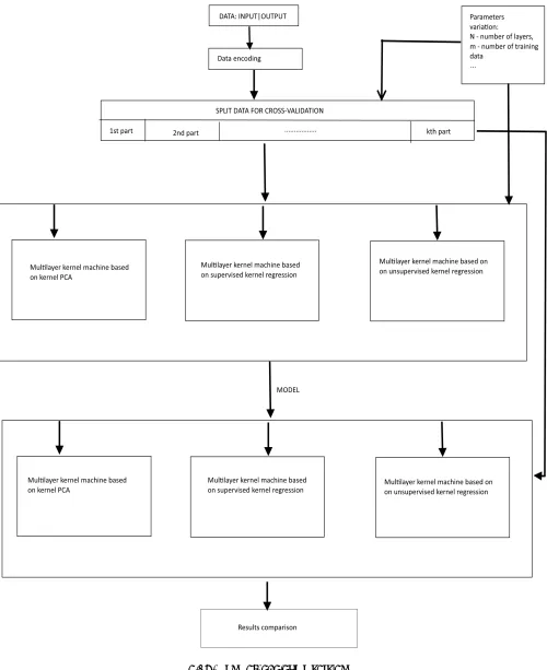
Error! Reference source not found. presents overview of the proposed methodology.

Figure 1. Methodology Overview

(4)

4

Figure. Multilayer kernels machine (MKMs) for the three different transformations

2.1. Multilayer RBF kernel machine based

on Kernel PCA

This Emphatically, the main concept in MKMs is the sequential transformation of input information using supervised feature selection, kernel PCA and unsupervised dimensionality reduction. This cycle above has meanwhile implemented the combined algorithm with unsupervised dimensionality reduction, iterate many times to formulate resulting multilayer kernel machines which incorporates unsupervised regression algorithm into kernel PCA to discard unwanted features.

Cho et al. (2009) described the first approach of multilayer kernel machine used in this work when he was developing an arc-cosine kernel that mimics the projections of a randomly initialized neural network.

This algorithm works in three processes: nonlinear transform by RBF kernel, unsupervised dimensionality reduction by kernel principal component analysis (PCA) and feature section by mutual information and this cycle is repeated multiple times to construct the feature hierarchy of MKM.

Below is a summary on how we implemented the Multilayer RBF machine based

on Kernel PCA and shown in Error! Reference source not found..

1. Let N be the number of layers we would like to use. 2. Prune the features by ranking method removing

redundant features.

3. Select appropriate kernels and kernel parameters (cross-validation or otherwise) –Apply kernel PCA algorithm and make the result be next layer set of features.

4. Determine number of features to extract prune the redundant features from the resulting.

5. If number of iterations exceeds N go to step 6, otherwise go to step 2.

6. Feed the feature representations to the classifier to make final decision.

The steps in the above procedures are standardized approach, but with novel combination. The promising outcome of the procedure is a justification to establish its implementation. We present below detailed discussion of the steps.

In kernel PCA, iterative application is employed to realize deep

(5)

5

learning in MKMs. Kernel PCA has been in existence since over ten years ago and now more newly inspired in an unsupervised approach through deep belief nets pre-training. The kernel PCA features in MKMs is used as input for next layer features. Meanwhile, in this case we select appropriate kernels and its parameters and apply from layer to the other. However, while nonlinear transform by arc-cosine kernel can be utilized in kernel PCA in MKMs, an RBF kernel that mimics the projections of a randomly initialized neural network is regarded an alternative approach, which is used in this work.

The idea of Cho (2012) is to implement unsupervised dimensionality reduction and supervised feature selection techniques into the multilayer arc-cosine kernels. However, in this work, the implementation of unsupervised dimensionality to reduce feature selection to exclude unwanted features or input into the next layer.

Kernel PCA features are best selected using ranking method in which redundant features are discarded. The ranking method is used to prune away inappropriate or unwanted features at each layer in the MKM. Naturally, the method helps to focus on the kernel PCA for deep learning. We prune features in just one-step, and then apply kernel PCA algorithm to produce a result that can be used as input for the next layer. Even from the obtained result, an optional option to prune selected features is employed to further minimize features redundancy. From the first step, we determine N number of layers to be used, and in step 6 we set loop of steps as long as the N number is not exceeded the second step of the algorithm will continue to iterate. We compute the result of the algorithm and feed the feature representations to the classifier to make final decision.

2.2. Multilayer RBF kernel machine based

on supervised kernel regression

This algorithm is extended from the first one by applying supervised kernel regression and removing the optional step of feature selection because it is done along with projection. Yger’s (2011) assume that it will give better computation time. For the latent arable regression, the feature extraction will also be incorporated in the regression step but it would be based not on the output but on the input. The author claims to overcome the drawback which is the step of feature selection by learning each hidden layer using Kernel Partial Least Squares regression (KPLS).

Below is a summary on how we implemented the Multilayer RBF machine based on supervised kernel regression and shown in Error! Reference source not found..

1. Let N be the number of layers we would like to use.

2. Select appropriate kernels and kernel parameters (cross-validation or otherwise) – not described in the work

3. Apply supervised regression to extract next feature value and corresponding Eigen value. 4. If Eigen value is greater than selected threshold go

to step 3 otherwise, use all the extracted features as input to the next layer.

6. Feed the feature representations to the classifier to make the final decision.

In this algorithm, feature selection methods and unsupervised dimensionality reduction is incorporated into supervised regression algorithm. In MKMs, deep learning approach is achieved through repetitive iteration of supervised regression algorithm sequentially list above. The use of this mean is however not new in this context, what is new here is how we apply the supervised regression with Eigen value to extract appropriate feature representative. Using the first algorithm, we have made a major contribution by replacing supervised regression with kernel PCA. We retained selection of appropriate kernel and kernel parameters, as they are already place from the existing algorithm. Since supervised training only occurs in the last layer in MKMs, this makes features selection method very important. From the first step, we determine N number of layer for this process. Like in the first algorithm for kernel PCA where ranking method is used to prune feature for appropriate selection. We then apply supervised regression to the pruned features. In supervised regression, the use of LMKMs is used to inspire deep learning training architectures. This is more specifically important achievement of the supervised regression algorithm used to extract next feature value and corresponding Eigen value.

The Eigen value is computed and determined through the algorithm steps any value greater than the threshold discarded. While appropriate value are all extracted as input for the next layer. The N number of layer we intend to use continue to iterate until number is greater than N. We feed the feature representations to implement the Multilayer RBF machine based on supervised kernel regression.

2.3. Multilayer RBF kernel machine based

on unsupervised kernel regression

This proposed algorithm based on unsupervised latent space and the motivation behind this claim is that unsupervised methods work well with the regular neural networks and unsupervised learning focusing on important patterns from data regardless of their labels as it reduces the input dimensionality of data without losing crucial information. In this algorithm we use the idea of unsupervised methods that is describe in Memisevic work (2003), which is Kernel parameters selection and dimensionality selection as shown in figure 3.

Let us say that we have data in q-dimensional space: 𝑌 ∈ 𝑅<_{(observable space), and we want to find the}

(6)

6

representation of this data in the d-dimensional space q>d: 𝑋 ∈ 𝑅>_{(latent space). Let us say we have N data points.} There are 2 types of unsupervised kernel regression for this purpose:

1. Optimize an error in the observable space.

𝐸@AB _{𝑋 =} _𝑦

2

-𝐾(𝑥2, 𝑥D)𝑦D E

DFG

𝐾(𝑥2, 𝑥H) E HFG I E 2FG • Advantages:

− We can use any kernel bandwidth h because it is easily replaced by the scale of the X.

• Disadvantages:

− We have very computationally consuming optimization problem with large number of parameters (N).

− We do not have explicit representation of x in terms of y which we will need to proceed with classification of new points.

2. Optimize an error in the latent space.

𝐸JKL _{𝑋 =} _𝑥

2

-𝐾(𝑦₂, 𝑦_D)𝑥_D E

DFG

𝐾(𝑦2, 𝑦H) E HFG I E 2FG • Advantages:

− There is an efficient way to solve this problem via eigen value decomposition. − We have explicit representation of x in

terms of y: 𝑥 = QORSM(N,NO)PO M(N,NT) Q

TRS , the solution depends on the selected kernel bandwidth which can be explained in the following steps :

1. For train set Y, find the solution X which optimizes error in the latent space. 2. For particular X and Y solve the

optimization problem to find optimal X scaling S (X:=X*S) which optimizes error in observable space.

3. Identify the optimal range for the h (kernel bandwidth) based on the graph connectivity algorithm.

4. Perform the algorithm of traversing through different values of h to identify the optimal one.

5. Select appropriate number of parameters d.

6. Write the code to incorporate method into classification.

7. Run the tests.

8. Add the special constraints concerning distances between different classes in the optimization problem to better fit the data for further classification. Adapt the optimization solution.

9. If results are unsatisfactory try the optimization in the observable space:

a. Determine X for train Y

b. Find the model for finding X for new points Y.

The idea of unsupervised kernel dimension reduction has been applied in [52] focusing on both linear and nonlinear unsupervised kernel dimension reduction. However, this current work has considered non-linear unsupervised kernel dimension reduction inspired by [52].

The kernel choice from [29] which is a Multilayer kernel machine (MKM), a kernel based model is adopted for the three algorithms experimented in this work. Particularly, MKM is introduced in the first algorithm to integrate unsupervised dimensionality reduction with supervised feature selection methods into kernel PCA algorithm.

Below is a summary of how we implement the Multilayer RBF machine based on unsupervised kernel regression and shown in Error! Reference source not found..

1. Let N be the number of layers we would like to use.

2. Apply unsupervised regression to extract latent variables which better represent the input parameters. (Kernel parameters selection and dimensionality selection is embedded in this step) based on the ideas described in the Memisevic work in Memisevic (2003)

- Learning of optimal latent space representation with input data

- Learning of transformation from observable to latent space.

- Selection of the kernel parameters and optimal dimensionality of the latent space

3. Use extracted latent variables as input to the next step.

5. Feed the feature representations to the classifier to make the final decision.

This algorithm combined both KPCA and supervised regression algorithm. This is done to achieve a more reliable input and consequently, results. An unsupervised regression algorithm is embedded with supervised feature selection and unsupervised dimensionality reduction. The idea of multilayer kernel machines (MKMS) implemented in this work is to help filter only feature relevant input, to be fed into developed unsupervised regression algorithm, and construct an infinite dimensional representation. Additionally, to help obtain result, unsupervised dimensionality reduction is implemented with feature space.

The attempt to adopt this approach is considered to be high level implementation concept of MKMs through the use of different machine learning techniques, which is this case a combination of two is used to develop another.

The implementation of the multilayer RBF machine based on kernel PCA is not new. However, in this algorithm, we

(7)

7

have replaced PCA with unsupervised kernel regression. The idea of unsupervised regression application is suggested by Memisevic (2003). The steps involved in the above algorithm are discussed. Based on Memisevic (2003) idea, this work combined feature selection with unsupervised regression. Unlike supervised regression procedure, latent variables are extracted instead using unsupervised regression method. In this work, we extract these variables my applying the input to obtain even better input parameters. This is equally based on three key steps

from Memisevic (2003). As usual, we determine N number of layer we want to use. As we are dealing with number of layers, previous output of the extracted latent variables are used as input to next layer. This process continues until the N number is reached. We then feed the feature representations to implement the multilayer RBF machine based on this algorithm for unsupervised kernel regression. The procedure of unsupervised regression method provided below in

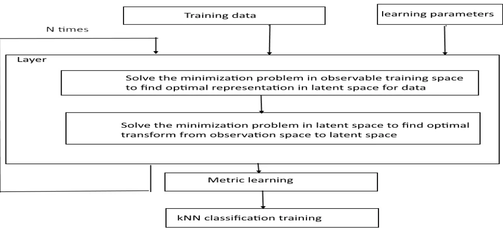
Figure 1.

Figure 1: The procedure of unsupervised regression (before improvement)

Unfortunately, after model training and evaluation of the three algorithms; the unsupervised method did not give a good accuracy as expected. In order to improve performance, the unsupervised latent regression with projection method is suggested.

The classifier based on this method is built by the following steps:

1. The whole training dataset is subdivided into several groups based on the data class labels. 2. For each group individually we train the following

model:

a. 𝑥 = 𝑔 𝑦 = QORSM(N,NO)∙PO M(N,NT) Q

TRS ; = 𝑓 𝑥 =

M(P,P_O)∙N_O Q

ORS M(P,PT) Q

TRS , where 𝐾 𝑎, 𝑏 is a kernel function.

b. The kernel is selected from the class of the multilayer RBF kernels.

c. The 1-layer RBF kernel is: 𝐾 𝑥, 𝑦 = 𝑒-,∙X,S P-N,, the combination of the RBF kernel K(𝑥, 𝑦)with kernel 𝐾G(𝑥, 𝑦) will be 𝐾 𝑥, 𝑦 = 𝑒G&X,SMS(P,N) _{. The goal of} the training is to define the values of the hyper parameters for each kernel. d. The optimal values of the particular

kernel are defined via eigenvalues decomposition problem as previously was done for the unsupervised latent regression. Then for these computed values the observable space error is defined as: 𝐸 = E2FG 𝑦2-𝑓(𝑔 𝑦2 ) , the built in cross-validation is used, meaning that 𝑦2 and 𝑥2 are excluded from the prediction stage. 𝑓 𝑥₂ =

M(P_Y,P_O)∙N_O Q

ORS,OZY

M(P_Y,P_T) Q

TRS,TZY , 𝑔 𝑦2 =

M(N_Y,N_O)∙P_O Q

ORS,OZY

M(N_Y,N_T) Q

TRS,TZY .

(8)

8

3. The points for which we want to predict the class label are processed via model 𝑓(𝑔 𝑦 ) to find the projection error for each group. The class giving minimum projection error is selected as a class label.

3. Practical Implementation

In this section we plan to compare multilayer kernel machines with different approaches for feature selection and dimensionality reduction. That means we will change steps 3 and 4 of the described method (supervised feature selection and unsupervised dimensionality reduction) and see how these changes affect the performance of the classification.

The major points for comparison:

1. Overall classification accuracy on different dataset: we are going to compare machines with same number of layers and equivalent kernel parameters.

2. Compare change of the classification performance with increased number of layers to answer these questions:

- How much the performance improves with addition of each new layer?

- What the limit number of layers the performance stops improving? 3. Compare how performance varies depending

on the number of training examples. 4. Compare computational complexity.

In order to achieve these goals; some requirements have been followed:

1. We use the same classification algorithm for all 3 methods: k-nearest neighborhood (KNN) classification algorithm with Mahalanobis distance metric learning used in [1] and described in [4].

2. We perform k-fold cross-validation: the input data are subdivided into k pieces on each iteration single piece of data is used for validation while other data are used for training in all 3 algorithms. As a result, a precision and recall was computed for all methods and number of selected features. 3. We change different parameters of the

method to see how the results of classification will change:

- Number of layers (How much the performance improves with addition of each new layer; are there any limits for number of layers: the number of layers after which the performance stops improving).

- Number of training examples

4. Experimental Results

4.1. Dataset Description

In these experiments, we work with three different datasets to assess the approach that has been proposed to make result comparison. The adopted datasets are;

1. The Apnea-ECG Database

This dataset obtained from Apnea-ECG database is with ECG signals for sleep apnea annotations. It has been selected also to validate the proposed approach in this work. The dataset in Apnea-ECG database contains 70 recordings of ECG for different patients with the range of 7 to 10 hours altogether. Meanwhile, just 35 recordings out of the 70 has minutes-wise apnea annotations. This suggests that apnea maybe occurs during each minute of ECG-data. However, only these 35 have been considered in the research.

4.2. Performance Metrics

In order to achieve the robustness of the results we used the 10-fold cross validation. All the points from the dataset selected for evaluation were:

1. Randomly permutated

2. Subdivided into 10 groups of equal size. The prediction algorithms were sequentially applied to each of these 10 groups while the others 9 were used to train the prediction model. The quality metrics were computed for each iteration and the averaged in order to achieve final results.

The following metrics are measured to evaluate the performance:

• Accuracy: is the ratio of correctly classified data points to the total number of data points

• Mean squared error (MSE):is the ratio of misclassified data to total number of data points

• Training time: is time in seconds which were

solely used to train the model on specific amount of data with predefined number of layers.

• Prediction time: is the time in seconds spent

solely on the prediction step with pre-trained model containing specific number of steps with fixed amount of training data.

4.3. Results Discussion and Analysis

The Apnea-ECG data set

(9)

9

For the Apnea-ECG database, we observe no significant change in both specificity and sensitivity values for all 5 layers. The impressive time results shown for training and validation times means this appears to be the best algorithm for best result in this respect. The improvement in the time parameters is achieved through limiting the number of features selected after projection. Unlike the previous two datasets, the Cohen kappa shows unaffected values through the 5 layers.

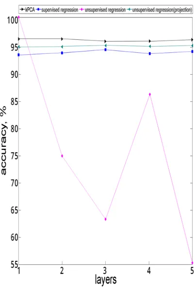
Figure 2 below presents the accuracy values for the four algorithms according to variation in number of layers.

Figure 2: Accuracy vs. number of layers when applying the four algorithms for Apnea dataset

Figure 3 below presents the MSE values for the four algorithms according to variation in number of layers.

Figure 3: MSE vs. number of layers when applying the four algorithms for Apnea dataset

Figure 4 below presents the sensitivity values for the four algorithms according to variation in number of layers.

Figure 4: Sensitivity vs. number of layers when applying the four algorithms for Apnea dataset

Figure 5 below presents the specificity values for the four algorithms according to variation in number of layers.

(10)

10 Figure 5: Specificity vs. number of layers when

applying the four algorithms for Apnea dataset

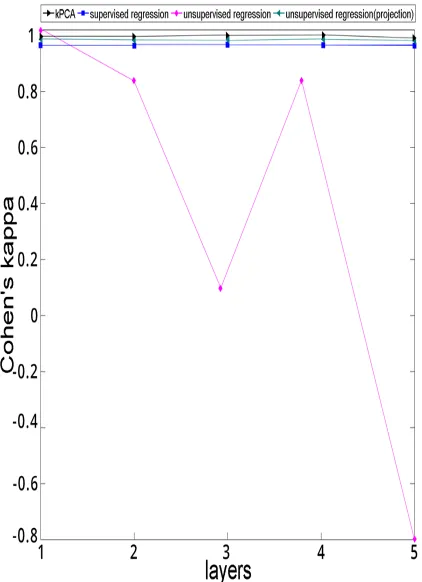
Figure 6 below presents the Cohen’s Kappa values for the four algorithms according to variation in number of layers.

Figure 6: Cohen’s Kappa vs. number of layers when applying the four algorithms for Apnea dataset

Figure 7 below presents the Training time values for the four algorithms according to variation in number of layers.

Figure 7: Training time (sec) vs. number of layers when applying the four algorithms for Apnea dataset

Figure 8 below presents the Validation time values for the four algorithms according to variation in number of layers.

Figure 8: Validation time (sec) vs. number of layers when applying the four algorithms for Apnea dataset

5. conclusion

In conclusion, the multilayered systems generally show relatively better results with large and highly varied data, as compared with “shallow learning” algorithms with usually single layer architecture. Moreover, amongst the multilayer algorithms, Supervised Regression tends to produce more stable and accurate results. As such, the usage of this particular algorithm should be

(11)

11 given greater consideration when conducting machine learning tasks involving large data sets and non-linear functions.

References

[1] Orr M. J. L. Introduction to radial basis function network. 1996 http://www.cc.gatech.edu/~isbell/tutorials/rbf-intro.pdf

[2] Orr M.J.L Recent advances in radial basis function networks. 1999

[3] http://www.anc.ed.ac.uk/rbf/papers/recad.ps

[4] Kubat M. Decision trees can initialize radial basis function networks

[5] http://citeseerx.ist.psu.edu/viewdoc/download?doi=10.1.1. 43.6674&rep=rep1&type=pdf

[6] Broomhead D.S., Lowe D. Multivariable functional interpolation and adaptive networks. 1998

[7] http://sci2s.ugr.es/keel/pdf/algorithm/articulo/1988-Broomhead-CS.pdf

[8] Schwenker F., Kestler H. A., Palm G. Three learning phases

for radial-basis-function networks. 2001

http://sci2s.ugr.es/keel/pdf/specific/articulo/skg01.pdf [9] T. Kohonen (1995), "Learning vector quantization", in

M.A. Arbib, The Handbook of Brain Theory and Neural Networks, Cambridge, MA: MIT Press, pp. 537–540 [10] Schwenker F., Kestler H.A., Palm G. 3-D Visual Object

Classification with Hierarchical Radial Basis Function

Networks.

http://www.uni-ulm.de/fileadmin/website_uni_ulm/iui/Ulmer_Informatik_ Berichte/2001/UIB_2001-02.pdf

[11] Cortes C., Vapnik V. Support-vector networks, 1995. http://image.diku.dk/imagecanon/material/cortes_vapnik95 .pdf

[12] Weston J., Watkins C. Multi-class support vector machines. http://citeseerx.ist.psu.edu/viewdoc/download?doi=10.1.1. 50.9594&rep=rep1&type=pdf

[13] Wettschereck D., Dietterich D. Improving the performance of the radial basis function networks by learning center locations.

[14] http://papers.nips.cc/paper/544-improving-the- performance-of-radial-basis-function-networks-by-learning-center-locations.pdf

[15] Chen S., Grant P.M., Cowan C. F. N. Orthogonal least-squares algorithm for training multi-output radial basis function networks. 1992.

https://cours.etsmtl.ca/sys828/REFS/B3/Chen_IEEE1992.p df

[16] Gomm B.J., Yu D.L. Selecting radial basis function network centers with recursive orthogonal least-squares training. 2000.

[17] http://ieeexplore.ieee.org/xpl/login.jsp?tp=&arnumber=839 002

[18] De Castro L. N., Von Zuben F. J. An immunological approach to initialize centers of radial basis function neural networks. 2001.

http://www.dca.fee.unicamp.br/~vonzuben/research/lnunes _dout/artigos/cbrn01.pdf

[19] Yousef R., el Hindi K. Training radial basis function networks using reduced sets as center points. http://citeseerx.ist.psu.edu/viewdoc/download?doi=10.1.1. 131.4275&rep=rep1&type=pdf

[20] Vachkov G., Stoyanov V., Christova N. Growing RBF network models for solving nonlinear approximation and classification problems. 2015.

[21]

http://www.scs- europe.net/dlib/2015/ecms2015acceptedpapers/0481-is_ECMS2015_0053.pdf

[22] Billing A.S., Zheng G.L. Radial basis function network configuration using genetic algorithms.

http://www.sciencedirect.com/science/article/pii/08936080 9500029Y

[23] Fasshauer G. E., Zhang J.G. On choosing “optimal” shape parameters for RBF approximation

[24] http://www.math.iit.edu/~fass/Dolomites.pdf

[25] Hoffman G.A. Adaptive transfer function in radial basis function (RBF) networks

[26] http://www.citemaster.net/get/a719201c-fb59-11e3-8a7f-00163e009cc7/hoffmann04adaptive.pdf

[27] Duch W., Jankowski N. Transfer functions: hidden

probabilities for better neural networks.

https://www.elen.ucl.ac.be/Proceedings/esann/esannpdf/es 2001-400.pdf

[28] Dorffner G. A unified framework for MLPs and RBFNs:

introducing conic section functions networks.

http://citeseerx.ist.psu.edu/viewdoc/download?doi=10.1.1. 49.7264&rep=rep1&type=pdf

[29] Mongillo M. Choosing basis functions and shape

parameters for radial basis function methods.

https://www.siam.org/students/siuro/vol4/S01084.pdf [30] Webb R.A. Shennon S. Shape-adaptive radial basis

functions

http://ieeexplore.ieee.org/xpl/login.jsp?tp=&arnumber=728 359

[31] Bengio Y., Courville A., Vincent P. Representation learning: a review and new perspectives

[32]

http://www.cl.uni-heidelberg.de/courses/ws14/deepl/BengioETAL12.pdf [33] Bengio Y., Delalleau O., Le Roux N. The curse of highly

variable functions for local kernel machines [34]

http://papers.nips.cc/paper/2810-the-curse-of-highly-variable-functions-for-local-kernel-machines.pdf

[35] Schmidhuber J. Deep learning in neural networks: an overview.

[36] http://www.sciencedirect.com/science/article/pii/S0893608 014002135

[37] Wang X. The application of deep kernel machines to various types of data.

[38] https://uwaterloo.ca/computational-

mathematics/sites/ca.computational-mathematics/files/uploads/files/shirly_project.pdf

[39] Bengio Y., LeCun Y. Scaling learning algorithms towards AI.

[40] http://cseweb.ucsd.edu/~gary/cs200/s12/bengio-lecun-07.pdf

[41] Bengio Y. Learning deep architecture for AI.

[42] http://www.iro.umontreal.ca/~bengioy/papers/ftml_book.p df

[43] Cho Y. Kernel methods for deep learning

http://citeseerx.ist.psu.edu/viewdoc/download?doi=10.1.1. 387.4491&rep=rep1&type=pdf

[44] LeCun Y., Bengio Y. Convolutional networks for images, speech and time-series.

[45] http://yann.lecun.com/exdb/publis/pdf/lecun-bengio-95a.pdf

[46] Erhan D., Courville A., Bengio Y., Vincent P. Why does unsupervised pre-training helps deep learning?

[47] http://www.dumitru.ca/files/publications/aistats_2010_cam era_ready.pdf

[48] Vincent P., Larochelle H., Lajoie I., Bengio Y., Manzagol P. A. Stacked denoising auto-encoders: learning useful

(12)

12 representations in a deep network using local denoising criteria.

[49] http://www.jmlr.org/papers/volume11/vincent10a/vincent1 0a.pdf

[50] Hinton G.E., Osindero S., Teh Y.-W. A fast learning

algorithm for deep-belief nets

https://www.cs.toronto.edu/~hinton/nipstutorial/nipstut3.p df

[51] Cho Y., Saul K. Large margin classification in infinite neural networks.

[52] http://cseweb.ucsd.edu/~yoc002/paper/neco_arccos.pdf [53] Bouvrie J., Rosasco L., Poggio T. On invariance in

hierarchical models.

[54] http://papers.nips.cc/paper/3732-on-invariance-in-hierarchical-models.pdf

[55] Bo L., Ren X., Fox D. Kernel descriptors for visual recognition

[56] http://www.cs.washington.edu/robotics/postscripts/kdes-nips-10.pdf

[57] Bo L., Lai K., Ren X., Fox D. Object recognition with hierarchical kernel descriptors

[58] http://www.cs.washington.edu/robotics/postscripts/hkdes-cvpr-11.pdf

[59] Mairal J., Koniusz P. , Harchaoui Z., Schmid C. Convolutional kernel networks.

[60] http://arxiv.org/pdf/1406.3332v2.pdf

[61] Zhuang J., Tsang I. W., Hoi S. C. H. Two-layer multiple kernel learning

[62] http://jmlr.csail.mit.edu/proceedings/papers/v15/zhuang11a /zhuang11a.pdf

[63] Bach R.F., Lankriet G.R.G. Multi-kernel learning, conic duality and the SMO algorithm

[64] http://www.di.ens.fr/~fbach/skm_icml.pdf

[65] Huang P.-S., Avron H., Sainath T.N., Sindhvani V., Ramabhadran B. Kernel methods match deep neural networks on TIMIT.

[66] http://www.ifp.illinois.edu/~huang146/papers/Kernel_DN N_ICASSP2014.pdf

[67] Strobl E.V., Visweswaran S. Deep Multiple kernel learning [68] http://arxiv.org/ftp/arxiv/papers/1310/1310.3101.pdf [69] Jose C., Goyal P., Aggrwal P., Varma M. Local deep kernel

learning for efficient non-linear SVM prediction [70]

http://research.microsoft.com/en-us/um/people/manik/pubs%5Cjose13.pdf

[71] Rebai I., BenAyed Y., Mahdi W. Deep multilayer multiple

kernel learning

http://link.springer.com/article/10.1007/s00521-015-2066-x

[72] Yger F., Berar M., Gasso G., Rakotomamonjy A. A supervised strategy for deep kernel machine

[73] https://www.elen.ucl.ac.be/Proceedings/esann/esannpdf/es 2011-21.pdf

[74] Welling M. Kernel principal component analysis http://www.ics.uci.edu/~welling/classnotes/papers_class/K ernel-PCA.pdf

[75] Ng A. Y., Jordan M.I., Weiss Y. On spectral clustering analysis and an algorithm

[76] http://ai.stanford.edu/~ang/papers/nips01-spectral.pdf [77] Welling M. Kernel canonical correlation analysis

http://www.ics.uci.edu/~welling/classnotes/papers_class/k CCA.pdf

[78] Wiering M.A., Schutten M., Millea A., Meijster A., Schomaker L.R.B. Deep support vector machines for regression problems

[79] http://www.ai.rug.nl/~mwiering/GROUP/ARTICLES/DSV M_extended_abstract.pdf

[80] Takeda H., Farsiu S., Milanfar P. Kernel regression for

image processing and reconstruction

http://people.duke.edu/~sf59/KernelRegression_Final.pdf

[81] Unsupervised kernel regression for non-linear

dimensionality reduction

http://www.iro.umontreal.ca/~memisevr/pubs/ukr.pdf [82] Memisevic R. Unsupervised kernel dimension reduction

http://www.cs.berkeley.edu/~jordan/papers/wang-sha-jordan-nips11.pdf

[83] http://deeplearning.net/datasets/

[84] https://archive.ics.uci.edu/ml/datasets.html [85] https://physionet.org/physiobank/database/#multi [86]