https://doi.org/10.5194/jsss-8-111-2019
© Author(s) 2019. This work is distributed under the Creative Commons Attribution 4.0 License.
Sensor characterization by comparative measurements
using a multi-sensor measuring system
Sebastian Hagemeier, Markus Schake, and Peter Lehmann
Measurement Technology Group, University of Kassel, 34121 Kassel, Germany
Correspondence:Sebastian Hagemeier ([email protected])
Received: 7 September 2018 – Accepted: 8 February 2019 – Published: 28 February 2019
Abstract. Typical 3-D topography sensors for the measurement of surface structures in the micro- and nanome-tre range are atomic force microscopes (AFMs), tactile stylus instruments, confocal microscopes and white-light interferometers. Each sensor shows its own transfer behaviour. In order to investigate transfer characteristics as well as systematic measurement effects, a multi-sensor measuring system is presented. With this measurement system comparative measurements using five different topography sensors are performed under identical con-ditions in a single set-up. In addition to the concept of the multi-sensor measuring system and an overview of the sensors used, surface profiles obtained from a fine chirp calibration standard are presented to show the diffi-culties of an exact reconstruction of the surface structure as well as the necessity of comparative measurements conducted with different topography sensors. Furthermore, the suitability of the AFM as reference sensor for high-precision measurements is shown by measuring the surface structure of a blank Blu-ray disc.
1 Introduction
The characterization of surface structures in the micro- and nanometre range can be done by various types of topogra-phy sensors. The demands on topogratopogra-phy sensors with re-gard to accuracy and measurement speed increase steadily. Currently the best-known method for three-dimensional to-pography measurement with respect to its transfer behaviour is the tactile stylus method, where the surface of the speci-men is scanned with a stylus tip. However, the tip may influ-ence the sample to be measured and also limits the measuring speed typically up to 1 mm s−1. Therefore, there are efforts to increase the measuring speed of tactile sensors and to reduce the wear of the stylus tip (Morrison, 1996; Doering et al., 2017). Doering et al. (2017) present a microprobe which al-lows tactile roughness measurements with a lateral scanning speed of 15 mm s−1.
Optical methods such as confocal microscopy, coherence scanning interferometry (CSI) and laser interferometry pro-vide an alternative (Jordan et al., 1998; de Groot, 2015; Schulz and Lehmann, 2013). The advantage of these methods is a fast and contactless measurement of the surface topogra-phy. Damages of the measuring surface as well as mainte-nance costs and measuring deviations due to worn probe tips
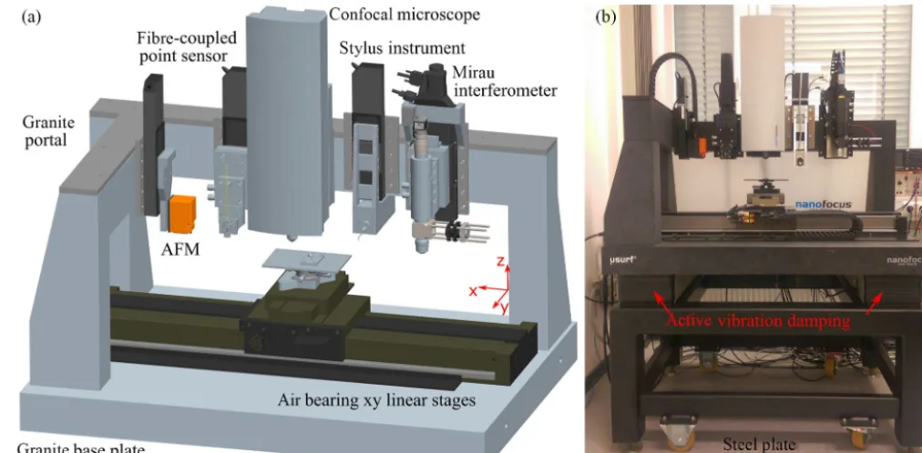
Figure 1.Schematic representation of the multi-sensor measuring system with five different topography sensors(a)and a photograph of the measuring system with active vibration damping on a steel plate reducing mechanical environmental vibrations(b).
(Hagemeier and Lehmann, 2018a). Next to the investigation of different systematic effects it is possible to characterize the transfer behaviour of our self-assembled topography sensors with this measuring system. A similar multi-sensor concept has already been pursued by Wiedenhöfer (2011) and Weck-enmann (2012). However, here the priority targets were the extension of the measuring range and the coverage of metro-logical requirements for different measuring objects through the use of different optical and tactile sensors.
2 Multi-sensor set-up
The multi-sensor measuring system comprises two self-assembled optical sensors (a Mirau interferometer and a fibre-coupled interferometric point sensor) as well as three commercial sensors (an atomic force microscope, AFM; a confocal microscope; and a tactile stylus instrument). The sensors are mounted on an L-shaped granite portal as shown in Fig. 1. Each sensor is connected to the granite portal by a vertically aligned linear stage. The linear stages provide a vertical positioning of each sensor in a range of 100 mm. With two horizontally aligned air bearing linear stages it is possible to position a specimen in the measuring vol-ume of the respective sensor. A lateral measurement field of 150 mm×100 mm is covered by all topography sensors for comparative measurements. In addition, the xy linear stages are used as scan axes for scanning a specimen surface horizontally as well as for stitching of several measurement fields. The repeatability of thexylinear stages is denoted by
±400 nm in thex direction and±50 nm in they direction. Based on this positioning accuracy it is possible to measure surfaces with stochastic structures without a reference point. In order to compensate for environmental vibrations, sev-eral techniques are employed. At higher frequencies vibra-tions are damped by the inertial mass of the granite used and the lower frequency spectrum is covered by an active vibra-tion damping system shown in Fig. 1b.
The atomic force microscope (AFM) can measure the sur-face in the tactile static mode and the contactless dynamic mode. In the more precise dynamic mode the maximum rms value of the noise of the measured height values is specified by 150 pm. The lateral deflection of the cantilever via three internally installed coils results in a maximum diamond-shaped measuring field of 110 µm×110 µm and a square field of 79 µm×79 µm. The maximum vertical deflection of the cantilever is 22 µm. Besides the low noise of the height values the lateral resolution of this sensor is much better than the resolution of optical sensors based on microscopic imag-ing, as demonstrated by measuring the surface of a Blu-ray disc in Sect. 3. For this reason, the AFM generates a precise surface topography of the structures to be measured and thus is qualified as a precision reference sensor for optical topog-raphy sensors.
Table 1.Scanning speed values and relatedRz0according to DIN EN ISO 3274 (1996), Lc=0.25 mm, Lc/Ls=100.
Rz0(nm) ≤30 ≤50 ≤80
vs(mm s−1) 0.1 0.5 1.0
camera. The depth scan required for the topography mea-surement is done by changing the distance between the mi-croscope objective and specimen by a stepwise motion of the objective using a piezoelectric-driven stage. At each step the camera detects an image of the surface. The confocal sensor provides a measurement field of 320 µm×320 µm by a total magnification of 23. At a numerical aperture (AN) of 0.95 the lateral optical resolution is approximately 320 nm using the Rayleigh criterion for conventional optical microscopy. By the confocal effect the lateral optical resolution is im-proved compared to classical light microscopy (Sheppard and Choudhury, 1977; Xiao et al., 1988; Wilson, 1990). As a result of the optical magnification and the pixel pitch of the camera the lateral sampling interval in the object plane is approximately 320 nm. Based on the Shannon criterion, grat-ing structures with a period larger than 640 nm can be recon-structed. The vertical resolution is specified with a noise level of 2 nm. To obtain an overview of the surface to be measured it is possible to generate conventional microscopic images besides the confocal measurement mode. Due to the high
ANand the different working principle compared to interfer-ometric sensors, the confocal microscope is an appropriate optical reference sensor.
The third reference sensor is the tactile stylus instrument. In particular, tactile measurements of surface contour and roughness can be obtained with this sensor. A stylus tip is brought into contact with the surface of the specimen and scans a line of 26 mm in theydirection with a scan velocity in a range of 0.1 to 1 mm s−1(for the coordinates see Fig. 1). Height differences of the surface structure result in deflec-tion of the tip which is measured. In combinadeflec-tion with thex
axis, several parallel profiles can be scanned and combined to a 3-D topography. The accuracy of the measured height information is specified by the residual valueRz0according to DIN EN ISO 3274 (1996); see Table 1.
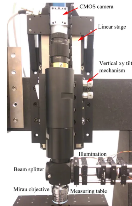
In addition to the three reference sensors, two different self-assembled interferometric topography sensors are inte-grated in the multi-sensor system. One of these 3-D sen-sors is the Mirau interferometer shown in Fig. 2. With this interferometer the transfer characteristics of white-light in-terferometers are investigated as an example, including the investigation of artefacts like the batwing effect (Xie et al., 2016, 2017). A special feature of this Mirau interferome-ter is its ability to simply adapt the spectral characinterferome-teristics of the light source and to perform depth scans of up to 100 mm using a stepper-motor-driven linear axis instead of an additional piezo-driven positioning system. Using a
lin-Figure 2. Self-assembled Mirau interferometer measuring a chirp standard provided by Physikalisch-Technische Bundesanstalt (PTB).
ear depth scan in combination with a CMOS camera with a USB3.0 interface, high-speed measurements are possible. At full resolution (2048 pixels×2048 pixels) the camera cap-tures 90 frames per seconds (fps) or 360 fps with a resolu-tion of 512 pixels×2048 pixels. For signal analysis differ-ent algorithms are used. In addition to the determination of the height values by detecting the position of the envelope, the more precise phase evaluation is inter alia obtained by a lock-in algorithm (LT algorithm) or frequency domain anal-ysis (Tereschenko, 2018; de Groot et al., 2002).
Figure 3.Fibre-coupled interferometric–confocal high-speed dis-tance sensor using a 1550 nm laser source.
a phase detection to calculate the height value h(x, y). Ne-glecting the offset, the two-beam interference equation takes the form
1I(t)=2pImIr cos
4π
λL
ˆ
zacos (2π fat)−h(x, y)
. (1)
Herezˆaandfarepresent the amplitude and frequency of the oscillating reference mirror. For each period of the oscillat-ing mirror, two height values result. Therefore, the oscilla-tion frequencyfaof 58 kHz used yields 116 000 height val-ues per second. This high acquisition rate allows a move-ment speed of the horizontal scan axis up to 100 mm s−1 as demonstrated using a sinusoidal standard (Hagemeier and Lehmann, 2018a). However, if a lower scan velocity is used, the high acquisition rate can be utilized to filter and improve the accuracy of the height values. In order to generate a 3-D topography of the surface to be measured, the air bearing
xy linear stages are used as scan axes. WithANof approx-imately 0.4, the lateral resolution is about 2.3 µm according to the Rayleigh criterion. However, the single-mode optical fibre acts as a pinhole of a confocal microscope (Kimura and Wilson, 1991; Gu and Sheppard, 1991; Dabbs and Glass, 1992), improving the lateral resolution and suppressing stray light.
3 Comparative measurements
At first, the result of a topography measurement on a blank Blu-ray disc (Verbatim BD-RW SL 25 GB) measured by the AFM is presented to underpin the suitability of this instru-ment as a high-resolution reference sensor. Figure 4 shows the measured topography as well as a 2-D profile of the struc-ture. The tracks of the Blu-ray disc with trapezoidal grooves
Figure 4.Topography and profile of a blank Blu-ray disc measured with the AFM (Hagemeier and Lehmann, 2018b).
Figure 5.Profile of the PTB chirp standard measured by the tactile stylus instrument GD26.
are well-resolved. The measured track pitch of 324 nm and groove depth of 24 nm correspond to the reported values of 320 and 20 nm (Meinders et al., 2006; Blu-ray Disc Asso-ciation, 2018; Lin et al., 2006). In order to be able to re-solve this fine surface structure, the cantilever EBD-HAR made of HDC/DLC (high-density carbon/diamond-like car-bon) by Nanotools is used. With an opening angle below 8◦ this cantilever is particularly suitable for measurements of steep edges and fine structures. The air bearingxylinear axes were also lowered prior to the measurement in order to mini-mize the influence of vibrations caused by the air stream. For comparison, a high-resolution Linnik interferometer with a
ANof 0.9 and a blue LED light source with a centre wave-length of 460 nm resolves the tracks of the disc too but not as detailed as the AFM (Lehmann et al., 2018).
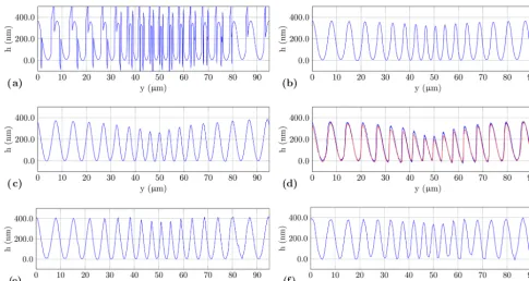
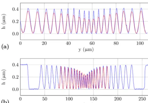
Figure 6.Profiles of the fine chirp structure obtained by various topography sensors:(a)50×Mirau interferometer with aANof 0.55 (phase evaluation using the LT algorithm) and a central wavelength of 590 nm,(b)unwrapped profile from(a),(c)confocal microscope,(d) high-speed sensor with two different scan velocities (blue: 0.1 mm s−1; red: 1 mm s−1),(e)AFM with a Tap190Al-G cantilever and(f)contact stylus instrument with a scan velocity of 0.5 mm s−1by using a probe according to DIN EN ISO 3274 (2 µm tip radius and an aperture angle of 60◦).
standard results from the profile measured by the tactile sty-lus instrument; see Fig. 5. The standard is divided into a coarse and a fine chirp structure. Both sinusoidal microstruc-tures are specified with a peak-to-peak amplitude of 400 nm. In the case of the coarse chirp the spatial wavelengths are in a range of 91 to 10 µm and in a range of 12 to 4.3 µm for the fine chirp (Brand et al., 2016). Such a chirp calibra-tion standard can be used to describe the transfer behaviour at different spatial wavelengths (Krüger-Sehm et al., 2007; Seewig et al., 2014). To represent the measured amplitude as a function of the spatial wavelength, the so-called instrument transfer function (ITF) can be used (de Groot and de Lega, 2006). With the knowledge about the real structure, the trans-fer function is estimated.
Figure 6a shows the measurement result of the Mirau in-terferometer withANof 0.55 and a magnification of 50×. In addition to the chirp structure, artefacts occur at the steep-est slopes of the structure. These artefacts are phase jumps caused by height displacements occurring as a result of en-velope evaluation, which in turn results from a too-low lat-eral resolution related to low-pass filtering of the fringes (Lehmann et al., 2016). By unwrapping this profile the phase jumps are removed as presented in Fig. 6b. This effect does not appear in the result of the confocal microscope, as it is shown in Fig. 6c. However, the profile indicates a stronger low-pass filtering of the structure compared to the Mirau
in-terferometer. When looking at the profiles, it is striking that there is only a one-sided constriction of the profile at the cen-tre. In theory, double-sided constrictions are to be expected in a low-pass-filtered profile. A possible reason for this ef-fect is indicated by an AFM measurement. Figure 6e shows the chirp profile measured by the AFM in the dynamic mode using a Tap190Al-G cantilever from BudgetSensors. Again, there is also a one-sided constriction with a height reduc-tion of approx. 40 nm. In addireduc-tion, the upper peaks of the sinusoidal structure in the centre of the chirp standard are tapered, resulting in a sharp-combed chirp structure. There-fore, the top levels are more affected by low-pass filtering compared to the bottom levels. To achieve high accuracy in the determination of the transfer behaviour of a topography sensor, the profile measured by AFM can be used as a refer-ence representing the original course of the chirp structure.
In the further three subsections the transfer behaviour of the tactile stylus instrument, the fibre-coupled high-speed sensor and the confocal microscope is investigated in more detail.
3.1 Tactile stylus instrument
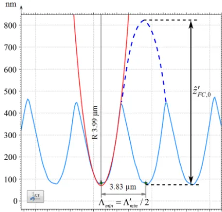
Figure 7.Section of the chirp profile with the shortest spatial wave-length measured by the AFM (blue line) and a fitted concentric cir-cle (red line) with a radius of 3.99 µm, using the software Moun-tainsMap. The additional blue dashed line illustrates a sine with the spatial wavelength30minand the amplitudezˆ0FC,0.
is used. Compared to the lateral resolution of the interfero-metric high-speed sensor (see Fig. 6d), similar low-pass fil-tering of the measured chirp structure is expected. However, the measured stylus profile in Fig. 6f shows a fairly good re-production of the reference structure. Deviations to the struc-ture measured by the AFM are inter alia formed by the lateral sampling distance of 0.5 µm, measuring deviations given by the residual value up to 50 nm according to Table 1 and the dilatation coming from the stylus tip. Due to the mechanical contact of the tip and the surface to be measured, no low-pass filtering of the upper tapered peaks appears and the real shape is reproduced nearly correctly.
The radius of curvature RFC,min at the smallest spatial wavelength 3min of the nominal sinusoidal chirp structure is
RFC,min=
32min
ˆ
zFC,0 4π2
≈1.83 µm, (2)
where 3min=3.8 µm (see Fig. 7) and the amplitudezˆFC,0 is equal to 200 nm. Because the structure is sharp-combed instead of sinusoidal, the radius of curvature of the grooves is assumed to be reasonably greater than 1.83 µm. This as-sumption is confirmed by the reference measurement of the AFM plotted in Fig. 7. Next to the area of the smallest spa-tial wavelengths (blue curve), a fitted concentric circle with a radius of 4 µm (red curve) is depicted, which was created using the analysis software MountainsMap. An explanation for the difference between the calculated value of 1.83 µm and the empirically determined value of 4 µm is given by the
sharp-combed structure. The sharp-combed profile almost re-sembles a rectified sine function of twice the period of the nominal sinusoidal chirp structure. Thus, the period30minof the sine to calculate the radiusR0FC,mincorresponds to twice the period3minwith twice the amplitude:
RFC0 ,min= 3
02 min
ˆ
z0FC,04π2=
32min
2zˆFC,0π2
≈3.7 µm, (3)
as it is graphically illustrated by the dashed blue line in Fig. 7. Hence, the grooves can be measured using a stylus instru-ment with a tip radius of 2 µm. In the case of an optical sen-sor, low-pass filtering of the structure occurs due to the lim-ited lateral-resolution capabilities, resulting in a double-sided constriction as a simulation shows (Schulz and Lehmann, 2016). On the other hand, when using a tactile measuring method, a one-sided constriction of the grooves is to be ex-pected, because the intrusion between two peaks is first lim-ited before the peaks are no longer resolvable.
In all measured profiles, the smallest period of the chirp structure is 3.8 µm. This leads to the conclusion that there is a deviation from the nominal sinusoidal structure of the 4.3 µm period.
3.2 Optical high-speed sensor
Median filtered profiles of the fine chirp structure obtained by the high-speed sensor with two different lateral scan veloci-ties (blue: 0.1 mm s−1; red: 1 mm s−1) are shown in Fig. 6d. Higher scan velocities such as 80 mm s−1are also possible as presented by Hagemeier et al. (2019). Both profiles of the high-speed sensor show a similar but stronger low-pass filter effect than the profile of the confocal microscope. In the pro-file measured at a higher scanning speed there is a stronger low-pass-filtering effect, which is due to an additional aver-aging over the surface heights caused by the scanning mo-tion. The sawtooth-like structure of both profiles is probably the result of a maladjusted sensor and needs further investi-gation.
In order to demonstrate the suitability of the measurement results of the AFM as a reference for the characterization of the transfer behaviour of the optical sensors, a simple exam-ple is presented in Fig. 8. To simulate the low-pass-filtering effect of the optical sensors a sliding average filter convolv-ing the profile with a rectangular function is used:
hc(ny1y)= 1
Nw
hafm(ny1y)·rect(ny1y), (4)
with the sampling interval1y, and a window length of the filterNw∈N,ny∈Nand
rect(ny1y)=
(
1 for 0≤ny1y≤1y(Nw−1) 0 for ny1y≥Nw1y.
Figure 8.Comparison of different profiles of the fine chirp struc-ture:(a)profile measured by AFM (blue) and the same profile fil-tered with a sliding average filter based on a rectangular impulse response function with a pulse width of 1.85 µm (red), and(b) com-parison of the filtered profile (red) from(a)and the structure mea-sured by the interferometric high-speed sensor (blue).
yields the best match for a width of the rectangular function ofNw1y=1.85 µm shown in Fig. 8a. Through the compari-son of this filtered structure with the profile measured by the interferometric high-speed sensor, a good congruence is ob-served, especially for the constriction of the upper and lower peaks; see Fig. 8b. A mathematical description of the focused laser beam of the high-speed sensor is possible assuming a Gaussian beam. Therefore, the minimal radius of the laser spot is equal to the smallest waistw0of the Gaussian beam (Kogelnik and Li, 1966):
w0=
λL
π arcsin (AN)
. (5)
For the high-speed sensor a minimum spot radius of 1.2 µm is therefore assumed. The half rectangular width used for the sliding filter corresponds to the radius of the laser spot and should be equal to 1.2 µm. However, the radius of the presented filtered structure (Fig. 8b) is approx. 0.9 µm. This is (about 25 %) smaller than the theoretical value. This dis-crepancy supports a smaller diameter of the laser spot and an accompanying improvement of the lateral resolution by the confocal effect caused by the single-mode fibre used. The scale of this value corresponds to the improvement (27 %) of the lateral single-point resolution between a con-focal and a conventional microscope described in Corle and Kino (1996). Besides small deviations in the determination of the filter width, a further reason can be a higher numeri-cal aperture. In addition, the result obtained by filtering the AFM profile confirms the theory of one-sided constrictions by low-pass filtering using optical topography sensors.
3.3 Confocal microscope
Using the confocal microscope with a numerical aperture
AN of 0.95 and an LED light source with a central wave-length λconf of 500 nm, a well-resolved profile of the fine chirp structure is expected. However, the Nyquist–Shannon sampling criterion is not satisfied by the equivalent camera pixel pitch of 320 nm, and the surface structure is not com-pletely resolved as shown in Fig. 6c. A first approach to in-vestigate the low-pass behaviour of the confocal microscope is to convolve the reference structurehafmmeasured by the AFM with the normalized point spread function (PSF) of the confocal microscope:
hc(y)=hafm(y)·PSFconf(y). (6)
Here, the PSFconfcorresponds to the square of the PSFconvof a conventional microscope (Sheppard and Choudhury, 1977; Martínez-Corral, 2003) and is described by
PSFconf(y)=PSF2conv(y)=
J1
2π λconfAN y
2π λconfAN y
4
, (7)
with the Bessel functionJ1of the first kind and order. Fol-lowing the convolution according to Eq. (6) the discretization due to the camera pixels is considered by an additional filter-ing accordfilter-ing to Eq. 4, whereNw1yis the equivalent pixel width of 320 nm. Therefore, everyNwth point is taken from the filtered result. As shown in Fig. 9a, there is a significant deviation between the filtered and the measured profile. A further approach is to rebuild the image formation. Appro-priate procedures are presented by Sheppard and Choudhury (1977) as well as Corle and Kino (1996) for confocal mi-croscopy using transmitted and reflected light. For the cal-culation of the intensities a simulation program introduced by Xie (2017) is used, which is based on the Richards– Wolf model (Richards and Wolf, 1959). Here, the measured AFM profile builds the input surface to rebuild the intensities
I(ny1y, nz1z) with the lateral sampling interval1y equal to 20 nm. The discretization of the camera pixels is achieved by averaging the resulting intensitiesIconf(y, z) covering a single camera pixel:
Iconf(l1ey, nz1z)= 1
Nw Nw
X
i=1
Iconf(l1y i, nz1z), (8)
with the pixel indexl∈N, the number of intensity samples
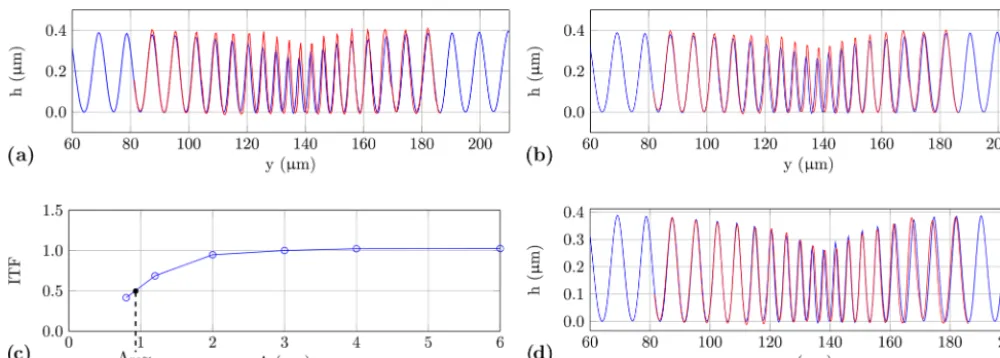
Figure 9.Transfer characteristics of the confocal microscope:(a)comparison of the chirp profile measured by confocal microscope (blue curve) and filtered profile according to Eq. (6) with an additional discretization by the camera pixels (red curve),(b)comparison of the measured profile of the confocal microscope (blue curve) to a reconstructed profile (red curve),(c)ITF resulting from the measured height of rectangular gratings with various spatial wavelengths in relation to the results of the AFM (see Table 2) with the spatial wavelength350 % equal to twice the spatial wavelength3Raccording to the Rayleigh criterion, and(d)comparison of the profile obtained with the confocal microscope (blue) and a filtered profile (red) according to Eq. (4) with a filter width of 33R.
Table 2. Comparison of height differences depending on various spatial period lengths3measured by AFM and confocal micro-scope using a RS-N standard manufactured by Simetrics.
3(µm) 6 4 3 2 1.2 0.8
hconf,pp(nm) 196 195 191 178 124 71 hAFM,pp(nm) 191 191 191 188 180 170
and can be a result of aberrations of the optical system which are not considered in the image formation model.
A favoured characterization of the transfer behaviour is given by the ITF, which describes the ratio of the measured and the true amplitude of a surface structure with respect to the spatial frequency. In the work of de Groot and de Lega (2006) the theoretical ITF is compared with experimental re-sults using a white-light interferometer to demonstrate the transfer behaviour for incoherent illumination as well as for coherent illumination by using a Fizeau interferometer. Fujii et al. (2011) compare multiple ITFs of a laser scanning con-focal microscope using various measurements on a chirp pro-file of different slope angles and amplitudes, using an AFM as reference instrument. A further application example is the characterization of a phase-shifting interferometer by an ITF created by measurements on a Siemens star with a structure height of about 50 nm (Giusca and Leach, 2013). A theo-retical investigation of the transfer behaviour of white-light interferometers using the ITF is given by Xie (2017).
In order to obtain the ITF, various measurements are per-formed with the confocal microscope on a Simetrics RS-N standard, as presented in Table 2. This standard covers
differ-ent rectangular gratings of various fundamdiffer-ental spatial fre-quencies3−1. The precision of the measured step height is increased by averaging 10 repeated measurement results for each spatial wavelength. As reference height, the measuring results of the AFM are used. The resulting ITF shows a de-crease below a grating period of 3 µm, as displayed in Fig. 9c. From the course of the curve a wavelength350 %of 925 nm is obtained, which is related to a decrease of 50 % of the real amplitude. As defined in DIN EN ISO 25178-604 (2013) and VDI/VDE 2655-1.3 (2018) for coherence scanning interfer-ometry,350 %equals twice the spatial wavelength3R pur-suant to the Rayleigh criterion:
350 %=2 3R=1.22
λconf
AN
χ . (9)
Based on the assumption that this relation is valid also for confocal microscopy,3Requals 462.5 nm. Ifχequals 1,3R corresponds to the theoretical optical lateral resolution ac-cording to the Rayleigh criterion. However, here the empiri-cal relation results in a multiplication withχ=1.45, which is a consequence of the deviation between the experimentally determined3Rand the theoretical optical resolution.
by optical aberrations of the confocal system due to imper-fect optical components and maladjustment.
4 Conclusions
The multi-sensor measuring system makes it possible to conduct comparative measurements with various sensors at equal environmental conditions. In addition to the determi-nation of the transfer characteristics of self-assembled sen-sors, the investigation of reference sensors is also possible. As a result of different working principles of the topography sensors used, artefacts or other deviations can be identified by comparative measurements. Since the measuring volume tracking is not fully implemented yet, the profiles shown in Fig. 6 are not measured on the exact same location on the specimen surface. For precise characterization of the trans-fer behaviour of a topography sensor, comparative measure-ments at equal locations are required. To reach this, further steps are essential. This includes the software implementa-tion of all sensors in a common C ++ program and the proper calibration of the spatial deviations between the individual locations of the measurement fields of the sensors. In ad-dition to positioning by the air bearingxy axes, the spatial conformity of the measurement fields can be increased by correlation of measured topographies. The desired maximum lateral deviation is 1 µm.
The accuracy of the height measurement of each reference sensor is characterized by different parameters for different instruments, namely the rms value for the AFM, the noise level for the confocal microscope and the residual valueRz0 for the stylus instrument. To ensure comparability, it is nec-essary to characterize both the individual reference sensors and the self-assembled topography sensors using the same parameter based on measurements on well-known surfaces.
As presented, the results of the AFM can be used as refer-ence data for the characterization of other sensors. For a the-oretical and numerical analysis of the measurement results of optical sensors, the results of the AFM can be used as input data to a simulation program introduced in Xie (2017), which is based on Kirchhoff theory and the Richards–Wolf model (Richards and Wolf, 1959).
Measurements at the same chirp structure using different topography sensors show the necessity of comparison mea-surements. Insight into the transfer behaviour of the sen-sors in the multi-sensor application is achieved by compar-ison of their chirp standard measurement results to those of the AFM. Therefore, the one-sided constrictions of the profiles measured by the optical sensors are explained by a sharp-combed structure instead of the originally assumed sinusoidal structure. Due to the sharp-combed structure the calculated nominal radius of curvature, based on the assump-tion of a sinusoidal structure, is too small. Thus the fine chirp profile is resolvable using the tactile stylus instrument with a tip radius of 2 µm. In spite of a lateral sampling interval
of 500 nm the structure of the chirp standard is almost cor-rectly measured. The presented comparative measurements between tactile and optical sensors indicate that depending on the surface structure of the measuring object, both tech-niques feature unique advantages, which are not available in a single-sensor system.
The multi-sensor measuring system is currently undergo-ing further development. As a final target, an automatic pro-cedure for comparative measurements is intended as well as the continuous testing and improvement of the topography sensors.
Data availability. The underlying measurement data are not pub-licly available and can be requested from the authors if required.
Competing interests. The authors declare that they have no con-flict of interest.
Special issue statement. This article is part of the special issue “Sensors and Measurement Systems 2018”. It is a result of the “Sen-soren und Messsysteme 2018, 19. ITG-/GMA-Fachtagung”, Nürn-berg, Germany, from 26 June 2018 to 27 June 2018.
Acknowledgements. The authors gratefully acknowledge the financial support of this project by the DFG (Deutsche Forschungs-gemeinschaft) under grant no. INST159/59-1 and thank the company Mahr for providing the stylus instrument GD26.
Edited by: Rainer Tutsch
Reviewed by: two anonymous referees
References
Blu-ray Disc Association: White Paper Blu-ray Disc format: Gen-eral, 5th Edition, available at: http://www.blu-raydisc.com, last access: 10 August 2018.
Brand, U., Doering, L., Gao, S., Ahbe, T., Buetefisch, S., Li, Z., Felgner, A., Meess, R., Hiller, K., Peiner, E., Frank, T., and Halle, A.: Sensors and calibration standards for precise hard-ness and topography measurements in micro-and nanotechnol-ogy, in: Micro-Nano-Integration; 6. GMM-Workshop; Proceed-ings of, 1–5 pp., VDE, 2016.
Corle, T. R. and Kino, G. S.: Confocal scanning optical microscopy and related imaging systems, Academic Press, 1996.
Dabbs, T. and Glass, M.: Fiber-optic confocal microscope: FOCON, Appl. Optics, 31, 3030–3035, 1992.
de Groot, P., de Lega, X. C., Kramer, J., and Turzhitsky, M.: Deter-mination of fringe order in white-light interference microscopy, Appl. Optics, 41, 4571–4578, 2002.
DIN EN ISO 25178-604: Geometrical product specification (GPS) – Surface texture: Areal – Part 604: Nominal characteristics of non-contact (coherence scanning interferometry) instruments, 2013.
DIN EN ISO 3274: Geometrical Product Specifications (GPS) – Surface texture: Profile method – Nominal characteristics of con-tact (stylus) Instruments, 1996.
Doering, L., Brand, U., Bütefisch, S., Ahbe, T., Weimann, T., Peiner, E., and Frank, T.: High-speed microprobe for roughness measurements in high-aspect-ratio microstructures, Meas. Sci. Technol., 28, 034009, https://doi.org/10.1088/1361-6501/28/3/034009, 2017.
Fewer, D., Hewlett, S., McCabe, E., and Hegarty, J.: Direct-view microscopy: experimental investigation of the dependence of the optical sectioning characteristics on pinhole-array configuration, J. Microsc., 187, 54–61, 1997.
Fujii, A., Suzuki, H., and Yanagi, K.: Development of measurement standards for verifying functional performance of surface texture measuring instruments, J. Phys. Conf. Ser., IOP Publishing, 311, 012009, https://doi.org/10.1088/1742-6596/311/1/012009, 2011. Giusca, C. L. and Leach, R. K.: Calibration of the scales of areal surface topography measuring instruments: part 3. Resolution, Meas. Sci. Technol., 24, 105010, https://doi.org/10.1088/0957-0233/24/10/105010, 2013.
Gu, M. and Sheppard, C.: Signal level of the fibre-optical confocal scanning microscope, J. Mod. Optic., 38, 1621–1630, 1991. Hagemeier, S. and Lehmann, P.: Multisensorisches Messsystem
zur Untersuchung der Übertragungseigenschaften von Topogra-phiesensoren (Multisensor measuring system for investigat-ing the transfer characteristics of topography sensors), tm-Technisches Messen, 85, 380–394, 2018a.
Hagemeier, S. and Lehmann, P.: Vergleichbarkeit des Über-tragungsverhaltens optischer 3D-Sensoren an Kanten und Mikrostrukturen (Comparability of the transfer behavior of 3D optical sensors at edges and microstructures), 2. VDI-Fachtagung Multisensorik in der Fertigungsmesstechnik, VDI-Berichte Nr. 2326, 199–212, 2018b.
Hagemeier, S., Tereschenko, S., and Lehmann, P.: High-speed laser interferometric distance sensor with reference mirror oscillating at ultrasonic frequencies, tm-Technisches Messen, https://doi.org/10.1515/teme-2019-0012, 2019.
Harasaki, A. and Wyant, J. C.: Fringe modulation skewing effect in white-light vertical scanning interferometry, Appl. Optics, 39, 2101–2106, 2000.
Jordan, H.-J., Wegner, M., and Tiziani, H.: Highly accu-rate non-contact characterization of engineering surfaces us-ing confocal microscopy, Meas. Sci. Technol., 9, 1142, https://doi.org/10.1088/0957-0233/9/7/023, 1998.
Kimura, S. and Wilson, T.: Confocal scanning optical microscope using single-mode fiber for signal detection, Appl. Optics, 30, 2143–2150, 1991.
Kiselev, I., Kiselev, E. I., Drexel, M., and Hauptmannl, M.: Noise robustness of interferometric surface topography evaluation methods. Correlogram correlation, Surface Topography: Metrol-ogy and Properties, 5, 045008, https://doi.org/10.1088/2051-672x/aa9459, 2017.
Kogelnik, H. and Li, T.: Laser beams and resonators, Appl. Optics, 5, 1550–1567, 1966.
Krüger-Sehm, R., Bakucz, P., Jung, L., and Wilhelms, H.: Chirp-Kalibriernormale für Oberflächenmessgeräte (Chirp calibration standards for surface measuring instruments), tm-Technisches Messen, 74, 572–576, 2007.
Lehmann, P., Tereschenko, S., and Xie, W.: Fundamental aspects of resolution and precision in vertical scanning white-light in-terferometry, Surface Topography: Metrology and Properties, 4, 024004, https://doi.org/10.1088/2051-672X/4/2/024004, 2016. Lehmann, P., Xie, W., Allendorf, B., and Tereschenko, S.:
Co-herence scanning and phase imaging optical interference mi-croscopy at the lateral resolution limit, Opt. Express, 26, 7376– 7389, 2018.
Lin, S. K., Lin, I. C., and Tsai, D. P.: Characterization of nano recorded marks at different writing strategies on phase-change recording layer of optical disks, Opt. Express, 14, 4452–4458, 2006.
Martínez-Corral, M.: Point spread function engineering in confocal scanning microscopy, SPIE Proceedings, 5182, 112–123, 2003. Mauch, F., Lyda, W., Gronle, M., and Osten, W.: Improved signal
model for confocal sensors accounting for object depending arti-facts, Opt. Express, 20, 19936–19945, 2012.
Meinders, E. R., Mijiritskii, A. V., van Pieterson, L., and Wuttig, M.: Optical Data Storage: Phase-change media and recording, vol. 4, Springer Science & Business Media, 2006.
Morrison, E.: The development of a prototype high-speed stylus profilometer and its application to rapid 3D surface measure-ment, Nanotechnology, 7, 37–42, https://doi.org/10.1088/0957-4484/7/1/005, 1996.
Richards, B. and Wolf, E.: Electromagnetic diffraction in optical systems, II. Structure of the image field in an aplanatic system, Proc. R. Soc. Lond. A, 253, 358–379, 1959.
Schake, M. and Lehmann, P.: Perturbation resistant RGB-interferometry with pulsed LED illumination, SPIE Proceedings, 10678, 1067805-01–1067805-12, https://doi.org/10.1117/12.2306221, 2018.
Schake, M., Schulz, M., and Lehmann, P.: High-resolution fiber-coupled interferometric point sensor for micro-and nano-metrology, tm-Technisches Messen, 82, 367–376, 2015. Schulz, M. and Lehmann, P.: Measurement of distance changes
us-ing a fibre-coupled common-path interferometer with mechan-ical path length modulation, Meas. Sci. Technol., 24, 065202, https://doi.org/10.1088/0957-0233/24/6/065202, 2013.
Schulz, M. and Lehmann, P.: Fasergekoppelter High-Speed-Sensor zum Messen optischer Funktionsflächen, 18. GMA/ITG-Fachtagung Sensoren und Messsysteme, 411–417, 2016. Seewig, J., Raid, I., Wiehr, C., and George, B. A.: Robust evaluation
of intensity curves measured by confocal microscopies, SPIE Proceedings, 8788, 87880T, https://doi.org/10.1117/12.2020551, 2013.
Seewig, J., Eifler, M., and Wiora, G.: Unambiguous evaluation of a chirp measurement standard, Surface Topography: Metrol-ogy and Properties, 2, 045003, https://doi.org/10.1088/2051-672X/2/4/045003, 2014.
Tereschenko, S.: Digitale Analyse periodischer und transienter Messsignale anhand von Beispielen aus der optischen Präzisions-messtechnik, Ph.D. thesis, University of Kassel, Germany, 2018. Tereschenko, S., Lehmann, P., Zellmer, L., and Brueckner-Foit, A.: Passive vibration compensation in scanning white-light interfer-ometry, Appl. Optics, 55, 6172–6182, 2016.
VDI/VDE 2655-1.3: Optical measurement of microtopography – Calibration of interference microscopes for form measurement, part 1.3, 2018.
Weckenmann, A.: Koordinatenmesstechnik: flexible Strategien für funktions-und fertigungsgerechtes Prüfen, Hanser, 2012. Wiedenhöfer, T.: Multisensor-Koordinatenmesstechnik zur
Erfas-sung dimensioneller Messgrößen, tm-Technisches Messen, 78, 150–155, 2011.
Wilson, T.: Confocal microscopy, Academic Press London, 1990. Xiao, G., Corle, T. R., and Kino, G.: Real-time confocal scanning
optical microscope, Appl. Phys. Lett., 53, 716–718, 1988.
Xie, W.: Transfer Characteristics of White Light Interferometers and Confocal Microscopes, Ph.D. thesis, University of Kassel, Germany, 2017.
Xie, W., Hagemeier, S., Woidt, C., Hillmer, H., and Lehmann, P.: Influences of edges and steep slopes in 3d interference and confocal microscopy, SPIE Proceedings, 9890, 98900X, https://doi.org/10.1117/12.2228307 2016.