http://www.sciencepublishinggroup.com/j/ijtam doi: 10.11648/j.ijtam.20170306.11
ISSN: 2575-5072 (Print); ISSN: 2575-5080 (Online)
He’s Homotopy Perturbation Method for solving Linear and
Non-Linear Fredholm Integro-Differential Equations
Bijan Krishna Saha
*, A. M. Mohiuddin, Sushanta Parua
Department of Mathematics, The University of Barisal, Barisal, Bangladesh
Email address:
[email protected] (B. K. Saha), [email protected] (B. K. Saha) *Corresponding author
To cite this article:
Bijan Krishna Saha, A. M. Mohiuddin, Sushanta Parua. He’s Homotopy Perturbation Method for solving Linear and Non-Linear Fredholm Integro-Differential Equations. International Journal of Theoretical and Applied Mathematics. Vol. 3, No. 6, 2017, pp. 174-181.
doi: 10.11648/j.ijtam.20170306.11
Received: April 29, 2017; Accepted: October 8, 2017; Published: November 10, 2017
Abstract:
In this paper, linear and non-linear Fredholm Integro-Differential Equations with initial conditions are presented. Aiming to find out an analytic and approximate solutions to linear and non-linear Fredholm Integro-Differential Equations, this paper presents a comparative study of He’s Homotopy perturbation method with other traditional methods namely the Variational iteration method (VIM), the Adomian decomposition method (ADM), the Series solution method (SSM) and the Direct computation method (DCM). Comparison of the applied methods of analytic solutions reveals that He’s Homotopy perturbation method is tremendously powerful and effective mathematical tool.Keywords:
Homotopy Perturbation, Variational Iteration, Adomian Decomposition, Series Solution, Direct Computation Method1. Introduction
Many researchers and scientists studied the integro-differential equations through their work in science applications like heat transformer, neutron diffusion, and biological species coexisting together with increasing and decreasing rates of generating and diffusion process in general. These kinds of equations can also be found in physics, biology and engineering applications, as well as in
models dealing with advanced integral equations such as [1-2], [22-23]. A new perturbation method called Homotopy perturbation method (HPM) was proposed in [8-19] by He in 1997, and a systematical description was given in 2000 which is in fact, a coupling of the traditional perturbation method and Homotopy in topology. This new method was further developed and improved by He and applied to various linear and non-linear problems.
= + , + , 0 = , 0 ≤ ≤ − 1 (1)
Where is the n-th derivative of the unknown function that will be determined, , is the kernel of the integral equation, is a known analytic function, and are linear and nonlinear functions of respectively. For
= 0 the equation (1) turn out to be a classical Fredholm differential equation. The Fredholm integro-differential equations (1) arise from the mathematical modeling of the spatiotemporal development of an epidemic model in addition to various physical and biological models and also from many other scientific phenomena. Nonlinear phenomena, which appear in many applications in scientific
solution for linear and nonlinear equations without any need for the so-called He's polynomials. Also this paper, will only focus on a brief discussion of He's Homotopy perturbation method because the details of the method are found in [8-19], and in many related works. For the sake of self-sufficiency of the article, the variational iteration method [7, 18-21], the Adomian decomposition method [5-6], the direct computation method (DCM) [3] and the series solution method [4] are reminded and employed for the comparison goal.
2. Materials and Methods
Homotopy perturbation method, Variational iteration method, Adomian decomposition method, series solution method, and Direct computation method have been applied to analyze the behavior of the solution of fredholm integro-differential equations. Finally a comparative study has been made among these methods.
2.1. Basic Idea of He’s Homotopy Perturbation Method
The Homotopy perturbation method (HPM) proposed by Shijun Liao in 1992 is based on the concept of the Homotopy, a fundamental concept in topology and differential geometry. Consider the nonlinear differential equation,
+ = , ∈ Ω (2)
With boundary conditions, " # ,$%$ & = 0, ∈ ' Where, L: A linear operator, N: A nonlinear operator, f(r): A known Analytic function, B: A boundary operator, ': The boundary of the domain Ω, By He’s Homotophy perturbation technique (He, 1999) Define a Homotopy ) , * :Ω× -0,1. → This satisfies
0 ), * = 1 − * - ) − . + *- ) + ) − . = 0, (3)
Or, 0 ), * = ) − + * + *- ) − . = 0, (4)
Where, ∈Ω, * ∈ -0,1. is an embedding parameter and is an initial approximation, which satisfies the boundary conditions. Clearly
0 ), 0 = ) − = 0,
0 ), 1 = ) + ) − = 0
As p changes from 0 to 1, Then v(r, p) changes from to . This is called a deformation and ) − ,
) + ) − are said to be Homotopy in topology.
According to the Homotopy perturbation method, the embedding parameter p can be used as a small parameter and assume that the solution of equation (3) and (4) can be expressed as a power series p, that is
) = ) + *) + *1)1+ … … … (5)
For p=1, the approximate solution of equation (1) therefore, can be expressed as
) = lim6→ ) = ) + ) + )1+ … … … (6)
The series in equation (6) is convergent in most cases and the convergence rate of the series depends on the nonlinear operator [Biazar and Ghazvini, 2009; He, 1999]. Moreover, the following judgments are made by He (1999, 2006)
1. The second order derivative of ) with respect to ) must be small as the parameter may be reasonably large, that is, * → 1
2. 7 8 #$9$:&7 Must be smaller than one, so that, the series converges
2.2. Variational Iteration Method
We consider the general n-th order integro-differential equations of the type [24]
; + ; + = , ;<
> = ? , @ < < (7)
With initial conditions
; @ =∝ , ;C @ =∝ , … … , ; 8 @ =∝
8 , (8)
Where ∝D, E = 0,1, … … , − 1, are real constants, m and n are integer and F < . In equation (7) the function f, g and k are given and y is the solution to be determined. Assume that the equation (7) has the unique solution. Here, change the problem to a system of ordinary integro–differential equations and apply the variational iteration to solve it, so that the Lagrange multiplier can be effectively identified. Using the following notation
; = ; ,GHGI= ;1,G
JH
GIJ= ;K, … ,G LMNH
GILMN = ; , (9)
Rewrite the integro-differential equation (7) as the system of ordinary integro-differential equations
GHN
GI = ; ,
GHJ
GI = ;K, GHO
GI = ;P, … … , GHL
GI = ? − ; − , ;<Q =
> (10)
With initial conditions
; ∝ =∝ , ;1 @ =∝ , ;K @ =∝1, … . , ; @ =∝ 8
To illustrate the basic concepts of the variational iteration method, consider the following differential equation
- . + - . = ? ,
Where L is a linear operator, N is a nonlinear operator and
g(x) is given continuous function. The basic character of the method is to construct a correction functional for the system, which reads
Q = + S->I + T − ? . , (11)
C+ U , C U = 0, S = −1,
CC+ U , C U , CC U = 0, S = U −
CCC+ U , C U , CC U , CCC U = 0, S = −1
2! U − 1,
… … … ..
+ U , C U , CC U , … , U = 0, S = −1
8 ! U − 8 ,
is the n-th approximate solution, and T denotes a restricted variation i.e, X T = 0. According to the variational iteration method, to solve the system (7), construct the
following correction functional
;Y Q = ;
Y + SI Y , -;YC − ;TYQ . , j=1, 2, …, n-1,
; Q = ; + Z SI , [;C − ? + ;T
+ Z= , \
> ;T<Q \ \] ,
Where the superscript (k) is the number of iterations steps. Calculating variation with respect to ;Y ^ = 1, 2, 3, … , respectively, and noting that X;Y = 0, We have
X;Y Q = X;Y + X Z SY , `;YC − ;TYQ a
I
> = X;Y + SY , X;Y |cdI− Z
eSY ,
e
I
> X;Y
= #1 − SY , & X;Y + Z f−eSYe , g I
> X;Y = 0, ^ = 1, 2, … . , − 1,
X; Q = X; + X Z S , [;C − ? + ;T
c + Z , \ ;T<Q \ \
=
> ]
I
>
= 1 + S , X; + Z f−I eSe , g
> X; = 0
For arbitrary X;Y , ^ = 1, 2, … . , , the following stationary conditions are obtained:
−$hNI,c
$c = − $hJI,c
$c = ⋯ = −
$hLI,c
$c = 0, (12)
And the natural boundary condition
1 + SY , = 0, ^ = 1, 2, … , .
The Lagrange multipliers therefore, can be identified as SY , = −1, ^ = 1, 2, … , . And the following iteration formula can be obtained as
;Y Q = ;Y − Z -;YC − ;YQ
I
> . , where ^ = 1, 2, … , − 1,
; Q = ; − -;I C − ? + ;
> + >= , \ ;<Q \ \. . (13)
Beginning with ; = n , ;1 = n , ;K =
n1, … ; = n 8 , by the iteration formula (13), we can
obtain the numerical solution of equation (7).
2.3. The Adomian Decomposition Method
The principal of the ADM when applied to a general nonlinear equation in the following form
+ + = ? (14)
Invers operator L, with 8 . = I . , equation (14) can be written as,
= 8 ? − 8 − 8 (15)
The decomposition method represents the solution of equation (15) as the following infinite series
= ∑p
d (16)
The nonlinear operator Nu=q is decomposed as
= ∑p r
d (17) Where r are Adomian polynomial which are defined as,
r = !GsGLLq-∑ tpDd D;D.sd = 1, 2, 3 … (18)
Substituting equation (16) and (17) into equation (15) we have,
= ∑ = 0 − 8 ∑p − 8
d p
d ∑pd r (19)
Consequently, it can be written as
= u + 8 , = − 8 − 8 r ,
2.4. The Series Solution Method
Assuming that u(x) is an analytic function, it can be represented by a series given by
= ∑p @
d , (20)
Where @ are constants that will be determined recursively. The first few coefficients can be determined by using the prescribed initial conditions where we may use
@ = 0 , @ = C 0 , @
1=2!1 CC 0 , ….
Substituting (20) into both sides of (7), and assuming that the kernel v , is separable as v , = ? ℎ ), obtain
∑pyd ayxy = + ? Iℎ { ∑pd @ + ∑pd @ | (21)
2.5. The Direct Computation Method
Assume a standard form to the fredholm integro-differential equation given by
= + v , , 0 = , 0 ≤ ≤ − 1 (22)
Where indicates the n-th derivative of u(x) with respect to x and are constants that define the initial conditions. This yield,
= + ? v , , 0 = , 0 ≤ ≤ − 1 (23)
It can easily observe that the definite integral in the integro-differential equation (18) involves an integrand that completely depends on the variable t, and therefore, it seems reasonable to set that definite integral in the right side of (23) to a constant α, that is we set
∝= ℎ . (24)
With α defined in (24), the equation (23) can be written by
= +∝ ? . (25) It remains to determine the constant n to evaluate the exact solution . To find α, we should derive a form for by using (25), followed by substituting this form in (24). To achieve this we integrate both sides of (25) n times from 0 to
x, and by using the given initial conditions
0 = , 0 ≤ ≤ – 1
Obtain an expression for given by
= * ; ∝ , (26) Where * ; n is the result derived from integrating (25) and by using the given initial conditions. Substituting (26) into the right hand side of (24), integrating and solving the resulting equation lead to a complete determination of α. The exact solution of (22) follows immediately upon substituting the resulting value of α into (26).
3. Results and Discussions
3.1. Solving the Following Linear Fredholm
Integro-Differential Equation by Different Methods
Example: Consider the Fredholm Integro-Differential equation
CCC = −•€\ + + Z CC ,
• J
0 = 0,
C 0 = 1, CC 0 = 0, (27)
3.1.1. Using He’s Homotopy Perturbation Method
A Homotopy can be readily constructed as follows
0 ), * = )CCC + •€\ − ‚ + •J )CC ,ƒ = 0 (28)
Substituting ) = ) + *) + *1)1+ … … into (28) and rearranging the resultant equation based on power of p-terms, one has
* : )CCC+ •€\ = 0, (29)
* : )CCC− − •J )CC = 0, (30)
*1 : )
1CCC− )CC
•
J = 0 (31)
and so on
With the following conditions
) 0 = 0,GcG) 0 = 0, = 1,2,3, … … (32)
With the effective initial approximation for ) from the conditions (32) and solution of (29), (30), (31) can be written as follows
) = „E ,
) = )1 = 0,
and so on.
In the same manner, the rest of components were obtained using the Mathemtica package
= lim6→ = ) + ) + )1 + … … … … (33)
Therefore, substituting the values of
) , ) , )1 @ )K in (33) yields
= „E . 3.1.2. Using Variational Iteration Method
In the view of variations iteration method, construct a correction functional for this equation (27) is given by,
Q = + S # CCC U + •€\U − U − U TCC
•
J & U
I
(34)
Where S is a Lagrange multiplier, therefore
S U = −1! U − 1. (35)
Now, the following variational iteration formula can be obtained
Q = −1! I U − 1 CCC U + •€\U − U−
U CC U
•
J (36)
We can use the initial condition to select = 0 +
C 0 +IJ
1! CC 0 =
Using this selection into the correction functional gives the following successive
Approximations
= ,
From (36) we have,
= − +4! + „E , P
1 =† K P
1152 −†
K P
1152 + †
ˆ P
27648 + „E ,
and so on.
The variation admits the use of = lim →p gives the exact solution = „E .
3.1.3. Using Adomian Decomposition Method
From (27) we have,
CCC = −•€\ + + •J CC , 0 = 0, C 0 = 1, CC 0 = 0, (37)
Applying the three-fold integral operator 8 defined by,
8 . = Z Z Z .
• J • J • J
To both sides of (37), that is integrating both sides of (37) thrice from 0 €Œ1, and using the given initial condition we obtain = „E +IP!•+IP!• CC
• J
Using = ∑pd and the recurrence relation we obtained,
= „E +4! , P = −4! +P †1152, K P
Similarly, 1 = −ŒOIŽ1•+1•ˆP‘Œ•I•,
and so on. This gives the solution in the series form,
= „E +4! −P 4! +P 1152 −†K P †1152 +K P 27648 + ’†ˆ P Ž
= „E
and this converges to the exact solution
= „E . 3.1.4. Using Series Solution Method
Equation (27) gives, CCC = −•€\ + +
CC ,
• J
0 = 0, C 0 = 1, CC 0 = 0, (38)
Substituting by the series
= ∑p @
d (39)
Using (39) in both sides of equation (38) we have,
“” @ p
d •
CCC
= −•€\ + + Z “” @ p
d • •
J CC
Differentiating the left sides twice and by evaluating the integral at the right sides
∑ − 1 − 2 @ 8K= #1 −IJ
1 + I•
1P− I•
•1 + … … & + + 2@1+ 6@K + 12@P 1+ 20@Ž K+ ⋯
• J
p
dK (40)
Using the initial condition and equating the coefficients of the powers of x in both sides of (40) gives the recurrence
@ = 0, @ = 1, @1= −2.43997, @K= −3! , @1 P= 0, @Ž
=5! , … …1
Substituting this results into, = ∑pd @ gives the series solution,
= „E − 2.43997 1.
This gives approximate solution.
3.1.5. Using the Direct Computation Method
We first set
n = •J CC (41)
So that given equation (27) can be written as
CCC = −•€\ + + n (42)
Integrating three times both sides of equation (42) we have
= „E +I1P•+—I1P•+˜NIJ
1 + ™1 + ™K (43)
Applying initial conditions in (43) we have
= „E + #1P+1P—& P (44)
Now we have n =P‘ −48 + †K− †Kn which gives
n = −1
By putting this value of n in (44) leads to the exact solution = „E .
3.2. Solving the Following Non-Linear Fredholm Integro-Differential Equation by Different Methods
Example:
C = •€\ −ŒI
P‘+1P 1 , Œ
0 = 0, n (45)
3.2.1. Using He’s Homotopy Perturbation Method
A Homotopy can be readily constructed as follows
0 ), * = )C − •€\ + * #ŒI
P‘−1P )1
Π& = 0
(46)
Substituting ) = ) + *) + *1)1+ … … into (46) and rearranging the resultant equation based on power of p-terms, one has
* : )C − •€\ = 0, (47)
* : )C +ŒI
P‘−1P )1 Œ
= 0, (48)
*1 : )
1C −1P Œ )1 = 0, (49)
and so on. With the following condition
) 0 = 0,
) 0 = 0,GcG) 0 = 0, = 1,2,3, … … (50)
With the effective initial approximation for ) from the conditions (50) and solution of (47), (48), (49) can be written as follows
) = „E , ) = )1 = ⋯ = 0,
In the same manner, the rest of components were obtained using the mathematica package
= lim6→ = ) + ) + )1 + … … (51)
Therefore, substituting the values of
) , ) , )1 r )K in (51) yields
= „E . 3.2.2. Using Variation Iteration Method
The correction functional for this equation (45) is,
Q = − Z
I
C U − •€\U + †
48 U
−24 Z U1 Œ U,
Where, S = −1 for first-order integro-differential equation. Using the initial condition to select = 0 = 0. This selection into the correction functional gives the following successive approximations
= 0,
= „E − 0.03272492349 1,
1 = „E − 0.000663791983 1,
K = „E − 0.00156723251 1,
and so on.
This gives the exact solution by
= „E − 0.0349559478 1.
3.2.3. Using Adomian Decomposition Method
From (45),
C = •€\ −ŒI
P‘+1P 1 , Œ
0 = 0, (52)
Applying the integral operator 8 defined by, 8 . =
.
I
To both sides of (52), that is integrating both sides of (52) from0 € , and using the given initial condition, which gives
= „E −ŒIšˆJ+ 8 #
1P 1
Π&
Using = ∑pd and the recurrence relation
= „E − 0.0327249 1
= 0.026087 1
= „E − 0.0327249 1+ 0.026087 1
+ 0.00420295 1+ … …
Thus = „E − 0.00243495 1
3.2.4. Using series Solution Method
From (45),
C = •€\ −ŒI
P‘+1P 1 ,
Π0 = 0
(53)
Substituting by the series
= ∑pd @ (54)
Using (54) in both sides of equation (53),
“” @
p
d
•
C
= •€\ −†48 +24 Z “” @1
p
d
•
Π1
Differentiating the left sides and by evaluating the integral at the right sides
∑ @ 8 = #1 −IJ
1 + I• 1P−
I•
•1 + … … & − ŒI
P‘+1P @ + @ + @1 1+ @K K+ @P P+ @Ž Ž+ ⋯
Πp
d (55)
Using the initial condition and equating the coefficients of the powers of in both sides of (55) gives the recurrence relation, @ = 0, @ = 1, @1= −2.43997, @K= −K!, @P=
0, @Ž=Ž!, … … … Substituting this results into, =
∑p @
d gives the series solution,
u x = Sinx − 2.43997x1.
3.2.5. Using the Direct Computation Method
First set,
n = Π1 (56)
So that given equation (45) can be written as
C = •€\ −ŒI
P‘+ —I
1P (57)
Integrating both sides of equation (57),
= „E −ŒIšˆJ+—IP‘J+ ™ (58)
Applying initial conditions in (58)
= „E − #96 −† 48&n 1
Thus from (56) and (58),
n =P‘ −48 + †K− †Kn (59)
Equation (59) gives, n = 2.11778. By putting this value of
n in (59) leads to the approximate solution
= „E + 0.0113954 1.
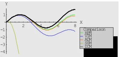
Figure 1. A Comparison of He’s Homotopy Perturbation Method and Traditional Methods for Solving Non-Linear Fredhlom Integro-Differential Equation.
C = •€\ −ŒI
P‘+1P 1 ,
Π0 = 0
.
4. Conclusion
This paper shows He’s Homotopy perturbation method of solving linear and non-linear Fredholm Integro-Differential Equation and conducted a comparative study between He’s Homotopy perturbation method and the traditional methods that is Variational iteration method, Adomian decomposition method, Series solution method and Direct computation method. The main advantage of the He’s Homotopy perturbation method are the fact that it provides its user with an analytical approximation, in many cases an exact solution in rapidly convergent sequence with elegantly computed terms. Also this method handles linear and non-linear equations in a straightforward manner. The four traditional methods suffer from the tedious work of calculation. Other traditional methods, that is usually used to solve integro-differential equations analytically and numerically, were not examined in this work, due to the huge size of calculations needed by these methods. Generally speaking, He's Homotopy perturbation method is convenient and more efficient compared to other techniques.
References
[1] A. J. Jerri, Introduction to Integral Equations with Applications, Marcel Dekker, New York, 1971.
[2] A. M. Golberg, Solution Methods for Integral Equations: Theory and applications, Plenum Press, New York, 1979. [3] A. M. Wazwaz, A First Course in Integral Equations, World
Scientific, 1997.
[4] F. G. Tricomi, Integral Equations, Dover, 1982.
[5] G. Adomian, Solving Frontier Problems of Physics: The Decomposition Method, Kluwer, 1994.
[6] G. Adomian, A review of the decomposition method and some recent results for nonlinear equation, Math. Comput. Model 13 (1992) 17_43.
[7] J. Biazar, H. Ghazvini, He's variational iteration method for solving linear and non-linear systems of ordinary differential equations, Appl. Math. Comput.191 (2007) 287_297.
2 4 6 8 X
-4 -3 -2 -1 1 Y
[8] J. H. He, Homotopy perturbation technique, Comput. Methods Appl. Mech. Engrg.178 (1999) 257_262.
[9] J. H. He, A coupling method of a homotopy technique and a perturbation technique for non-linear problems, Internat. J. Non-linear Mech. 35 (2000) 37_43.
[10] J. H. He, Homotopy perturbation method: A new non-linear analytical technique, Appl. Math. Comput.135 (2003) 73_79. [11] J. H. He, Comparison of homotopy perturbation method and
homotopy analysis method, Appl. Math. Comput.156 (2004) 527_539.
[12] J. H. He, Thehomotopy perturbation method for non-linear oscillators with discontinuities, Appl. Math. Comput.151 (2004) 287_292.
[13] J. H. He, Application of homotopy perturbation method to non-linear wave equations, Chaos Solitons Fractals 26 (2005) 695_700.
[14] J. H. He, Homotopy perturbation method for bifurcation of non-linear problems, Int. J. Non-linear Sci. Numer. Simul.6 (2005) 207_208.
[15] J. H. He, Periodic solutions and bifurcations of delay-differential equations, Phys. Lett.347 (2005) 228_230.
[16] J. H. He, Limit cycle and bifurcation of non-linear problems, Chaos Solitons Fractals 26 (2005) 827_833.
[17] J. H. He, Determination of limit cycles for strongly non-linear oscillators, Phys. Rev. Lett. 90 (2003) Art. No. 174301. [18] J. H. He, Variational iteration method-a kind of non-linear
analytical technique: Some examples, Int. J. Nonlinear Mech. 34 (4) (1999) 699_708.
[19] J. H. He, Variational iteration method Some recent results and new interpretations, J. Comput. Appl. Math. 207 (2007) 3_17. [20] LanXu, Variational iteration method for solving integral
equations, Comput. Math. Appl. 54 (2007) 1071_1078. [21] M. Tatari, M. Dehghan, On the convergence of He's
variational iteration method, J. Comput. Appl. Math. 207 (1) (2007) 121_128.
[22] R. P. Kanwal, Linear Integral Differential Equations Theory and Technique, Academic Press, New York, 1971.
[23] R. K. Miller, Nonlinear Volterra Integral Equations, W. A Benjamin, Menlo Park, CA, 1967.