Nonlin. Processes Geophys., 15, 601–606, 2008 www.nonlin-processes-geophys.net/15/601/2008/ © Author(s) 2008. This work is distributed under the Creative Commons Attribution 3.0 License.
Nonlinear Processes
in Geophysics
A new method for abrupt change detection in dynamic structures
W. P. He1,2, G. L. Feng1,2, Q. Wu3, S. Q. Wan4, and J. F. Chou5
1National Climate Center, China Meteorological Administration, Beijing, China
2Key Laboratory of Regional Climate-Environment for Temperate East Asia, Institute of Atmospheric Physics, Chinese Academy of Sciences, Beijing, China
3Chinese Academy of Meteorological Sciences, Beijing, China
4Yangzhou Meteorological Bureau of Jiangsu Province, Yangzhou, China 5Department of Atmospheric Sciences, Lanzhou University, Lanzhou, China
Received: 13 May 2008 – Revised: 30 June 2008 – Accepted: 30 June 2008 – Published: 24 July 2008
Abstract. Based on Detrended Fluctuation Analysis (DFA),
we propose a new method – Moving Detrended Fluctua-tion Analysis (MDFA) – to detect abrupt change in dynamic structures. Application of this technique shows that this method may be of use in detecting time-instants of abrupt change in dynamic structures and we even find that the MDFA results almost do not depend on length of subseries, and are less affected by noise.
1 Introduction
Abrupt change detection in meteorological area is a much studied subject (Alexi et al., 2007; Alley et al., 2003; Broecker, 2003; Ganopolski, et al., 2002; Rahmstorf, 2003; Thomas et al., 1988; Wunsch, 2006). It plays a significant role in improving climate prediction. There are various tra-ditional methods for approaching climate abrupt change de-tection such as moving t-test, Cramer Method, Yamamoto Method (Yamamoto et al., 1985) and Mann-Kendall test (Mann, 1945; Kendall et al., 1975). These methods have in common that detection results strongly depend on the length of subseries, namely analyzed timescales. Using these tra-ditional approaches, we find the detected time-instants of abrupt change are extremely different for different lengths of subseries. There are two types of abrupt change, one is caused by the change of dynamic equation, and the other is caused by the change of phase or evolution trend (or fre-quency) of a system but dynamic equation does not change. These traditional methods cannot distinguish the two types of abrupt change. In order to deal with this problem, Pin-cus (1993, 1995) proposed Approximate Entropy which is
Correspondence to: W. P. He (wenping [email protected])
generally called ApEn for short and could identify dynamic structure to some extent but still depend on the lengths of subseries. At the same time, there exists a huge drift for the ApEn results which means the actual time-instants of abrupt change don’t overlap with the detected one. Making sure of characteristics and time-instants of abrupt change is very im-portant for climate prediction. For that reason, it is essential to provide a new detection method to exactly solve this prob-lem.
Previous studies have shown that a large quality of time series exhibit scaling behaviors (Bunde et al., 2000, 2005; Cao, 1997, 2003; Jan et al., 2007; Liu et al., 2000; Livina et al.,2005; Peter et al., 2000), such as daily temperature records exhibit long-range correlation, which is character-ized by an infinite correlation time and linked to power-law behavior of autocorrelation function (Fraedrich et al., 2003), namely:
C(s)∼s−α,0<α<1. (1)
A power-law relationship betweenC(s)andsindicates scal-ing with an exponentα. Therefore, based on a scaling tech-nique, Detrended Fluctuation Analysis (DFA) (Peng et al., 1993, 1994), we propose a new abrupt change detection method – Moving Detrended Fluctuation Analysis (MDFA). It is mainly used to detect abrupt change in dynamic struc-tures. In this paper, we consider two types of abrupt dynamic structure change:
1. abrupt parameters change in systems;
2. abrupt change caused by external forcing or interactions between systems.
0 200 400 600 800 1000 0
2 4 6 0 2 4 6 -20 -10 0 10 20
L=300
p
n
L=200 IS0
p
(c) (b) (a)
no abrupt change
x
Fig. 1. (a) The IS0 time series x(i)(i=1, 1000) of 1000 units,
in which there is no abrupt change in dynamic structure; (b) the
MDFA4results of IS0, the length of subseries is equal to 200; (c)
same as Fig. 1b, but the length of subseries is equal to 300.
This paper is organized as follows: Sect. 2 describes the abrupt change detection methodMDFA and the data in tests, and then we provide the results and discussion in Sect. 3. Finally, our conclusions are presented.
2 Method and data
Estimating the autocorrelation functionC(s)from empirical data is limited to rather small lag s and is affected by obser-vational noise and nonstationarities such as trends (Maraun et al., 2004). Therefore, in this paper, we employ DFA, a scaling analysis method that can deal with seemingly non-stationary time series, and which provides a simple quanti-tative parameter – scaling exponent – to describe power law in time series (Peng et al., 1993, 1994). The relationships between scaling exponentsαandpare (Bunde et al., 2000, 2005; Maraun et al., 2004):
α=2(1−p). (2)
Different ordersnof DFA (DFA1, DFA2etc.) differ in the order of the polynomial used in DFA procedure (Monetti et al., 2003). Accordingly, different ordern of MDFA proce-dure can be marked by MDFAn. In order to detect abrupt
change in dynamic structures which exist in time series, we first choose a subseries to calculate a scaling exponent by DFA, and then move subseries gradually without changing the length of subseries, repeat this operation until the end of the original series. If there is an abrupt change in dy-namic structure, the scaling exponent will have a very sharp change in the vicinity of abrupt change. Whereas, if there is no abrupt change in dynamic structure, the scaling expo-nent will have a relative tiny change, and this change mainly caused by an insufficiency of samples size. Based on these characteristics, we can easily identify time-instants of abrupt change in dynamic structures. The data in tests come from
0 200 400 600 800 1000
2 4 6 0 4 8 -15 0 15
p
n
L=200 L=100
(c)
p
IS1
(b) (a)
x
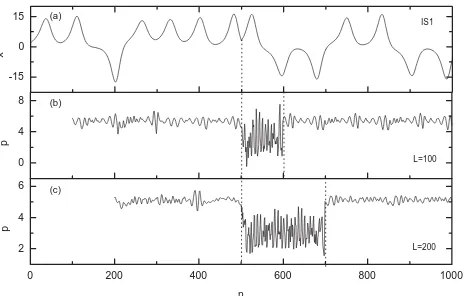
Fig. 2. (a) The IS1time seriesx(i)(i=1,1000) of 1000 units, in
which there is an abrupt change in dynamic structure whenn=501;
(b) the MDFA4results of IS1, the length of subseries is equal to
100; (c) same as Fig. 2b, but the length of subseries is equal to 200.
chaos model, such as classical Lorenz model (Lorenz et al., 1963) or Chen model (Chen et al., 1999), and the data dis-play scaling character. In this paper, all the lengths of model time series are 1000 units.
3 Results and discussion
Figure 1a shows a model time series IS0, which is produced by Lorenz system when Rayleigh parameter R=28.0, and there is no abrupt dynamic change in IS0. Figure 1b and c shows the MDFA4results for the model time series used in Fig. 1a. When the length of subseries is equal to 200, the maximum and minimum of scaling exponents is respectively 5.57343, 4.60895 and the variation of scaling exponents is about 0.96448. When the length increases to 300, the max-imum and minmax-imum of scaling exponents are respectively 5.14896, 4.55396 and the variation approximately decreases to 0.595. We use MDFA4 to detect other model time se-ries which have no abrupt dynamic change, and we find that the results are similar to that of IS0. The variation of scal-ing exponents is relatively small, which is a common char-acter for those model time series without abrupt dynamic change. Meanwhile, we find that the variation of scaling ex-ponents decreases with the increase of length of subseries. Consequently, for those time series without abrupt dynamic change, it is obvious that fluctuation of scaling exponents induced by moving subseries mainly due to the shortage of sample size.
To illustrate parameter change which induces abrupt change in dynamic structure, we use the model time series IS1 which is formed by the variable x in Lorenz system (see Fig. 2a). The previous half in IS1 are produced when Rayleigh parameterR=29.0, the others are produced when
W. P. He et al.: A new abrupt change detection method 603
0 200 400 600 800 1000
0.000 0.004 0.008 0.012 0.00 0.01 0.02 0.03 0.04
Variance contribution
(b)
Variance contribution Average of Variance contribution L=200
n (a)
Variance contribution Average of Variance contribution L=100
Fig. 3. Variance contributions of scaling exponents. (a) Variance
contributions for detection results of IS1 by using MDFA4, the
length of subseries is equal to 100; (b) same as Fig. 3a, but the length of subseries is equal to 200.
Figure 2b and c shows the MDFA4 results for the model time series IS1, respectively. According to the difference of fluctuation amplitude of scaling exponents, We can easily find from Fig. 2b that the evolution curve of scaling expo-nents can be roughly divided into three parts:
1. (100,500); 2. (501,600); 3. (601,1000).
In the first and third parts, the fluctuation of scaling expo-nents is stable, additionally fluctuation amplitude is relatively small and the variation is about 2.96393. As said before, the relatively small fluctuation amplitude mainly dues to the shortage of sample size. But in the second part, the fluctua-tion amplitude of scaling exponents increase apparently and the variation is about 7.99496. The reason is that MDFA is very sensitive to the data from different system. In other words, if subseries are comprised of data coming from differ-ent dynamic systems, the variation of scaling expondiffer-ents ap-parently greater than that of subseries, which are comprised of data coming from identical dynamic system. Figure 2b and c shows that MDFA4 can be used to detect the abrupt dynamic structural change in the model time series IS1.
To exactly give time-instants of abrupt dynamic change from the MDFA4results, we need present a quantitative mea-sure. In view of the sensitivity of MDFA to the data com-ing from different dynamic systems, in this paper, we esti-mate the time-instants of abrupt change quantitatively from the MDFA results according to the variance contribution of scaling exponents. It should be noted that the average of scaling exponents in variance contribution procedure is cal-culated by scaling exponents, the variation of which is rel-atively smaller. For example, when the length of subseries is 100, the average of scaling exponents for the model time
100 150 200 250 300 350 400 501
502 503 504 505 506
the time instant of abrupt change
Length of subseries
Fig. 4. The time-instants of abrupt dynamic change as a function of
length of subseries for IS1.
series IS1is calculated by the scaling exponents in the first and third parts in Fig. 2b. Figure 3a and b presents the results of variance contribution procedure of scaling exponents, ac-cording to Fig. 2b and c, respectively. We find that the plots of variance contribution can distinguish normal fluctuation amplitudes from abnormal ones. The normal one is mainly caused by the shortage of sample size, and the abnormal one is primarily caused by the sensitivity of MDFA to the data from different system. We define the time-instant of abrupt change is the point when the first variance contribution is above the average of variance contribution. Based on this definition, we find that all the time-instants of abrupt dy-namic change in IS1aren=503 when the lengths of subseries are respectively 100 and 200. Then we use MDFA4to analy-sis IS1for other different lengths of subseries, and the results have been shown in Fig. 4. It can be seen from Fig. 4 that the time-instant of abrupt change range from 501 to 506, which are all very close to the actual time-instant of abrupt change (n=501). The MDFA results indicate that MDFA can be used to effectively detect abrupt dynamic change, and hardly de-pend on the length of subseries. We can get similar results by using other orders of MDFA.
0 200 400 600 800 1000 2
4 6 0 4 8 -15 0 15
p
n
L=200 L=100
(c)
p
IS2
(b) (a)
x
Fig. 5. Same as Fig. 2, but the time series is IS2.
Table 1. The number of abrupt change in IS1for different lengths
of subseries by using traditional methods.
Traditional Method Length of subseries 100 200 300
Moving t-test 8 3 1
Cramer Method 5 1 0
Mann-Kendall 5 3 2
of length of subseries, there is a decreasing trend in the num-bers of abrupt change. The Yamamoto method cannot detect any abrupt change in IS1. The ApEn results indicate that the time-instant of abrupt change depends on the length of subseries, for example, the detected time-instants of abrupt change aren=181, 392, 487, 530 for the lengthL=100, 200, 300, 400, respectively. It is obvious that the performance of MDFA is better than that of traditional methods.
Model time series IS2is composed of two parts: the clas-sical Lorenz model (Lorenz et al., 1963) and the periodic forcing Lorenz model, which is as follows:
dx
dt=−σ x+σ y+Acos(wt ) dy
dt=Rx−y−xz dz
dt=xy−bz (3)
Ais the forcing strength, we get 0.005 here, Acos(wt ) is the forcing term.W is the frequency of periodic forcing, we get 0.02 here. Parametersσ, bare 10.0 and 8/3, respectively.
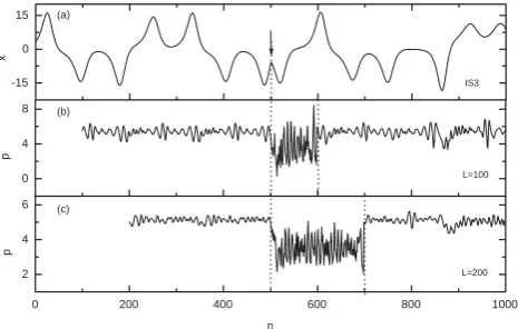
R is Rayleigh number, which is equal to 28.0. Figure 5a shows the evolution curve of the model time series IS2, and the first 500 data are produced by the variablex in classic Lorenz equations, the others are produced by the variablex
in Eqs. (1). Figure 5b and c show the MDFA4 results for different lengths of subseries. Based on variance contribu-tion procedure (Figs. omit), we find that the time-instant of abrupt change is n=504, which is very close to the actual
0 200 400 600 800 1000
2 4 6 0 4 8 -15 0 15
p
n
L=200 L=100
(c)
p
IS3
(b) (a)
x
Fig. 6. Same as Fig. 2, but the time series is IS3.
time-instant of abrupt change. The model time series IS2 is very smooth, and so it is usually difficult to find out the time-instant of abrupt dynamic change. But we can easily and exactly detect the time-instant of abrupt change through MDFA4.
Climate system includes various kinds of subsystems. There exists coupling between different climate systems, sometimes it is strong and sometimes it is weak. A coupling can be ignored when its coupling strength is weak, however, it cannot be ignored when its coupling strength is strong. The strong interactions between subsystems may induce the evolution of climate system to an exceptional state, such as floods, drought, extreme high temperature etc. We now consider a simple binary model and its strong interactions between subsystems have caused abrupt dynamic change. This model is composed of Lorenz model and Chen system (Lorenz et al., 1963; Chen et al., 1999), the coupling binary model can be written as:
dx1
dt = −σ x1+σ y1+E(x1−x2) dy1
dt =r1x1−y1−x1z1 dz1
dt =x1y1−b1z1 dx2
dt = −ax2+ay2+w2−E(x1−x2) dy2
dt =dx2+cy2−x2z2 dz2
dt =x2y2−b2z2 dw
dt =y2z2−r2w (4)
x1, y1, z1 are three variables of Lorenz model, respec-tively, and x2, y2, z2, w are four variables of Chen sys-tem. E(x1−x2)is the coupling term. The two subsystems can achieve interactions through coupling between variable
W. P. He et al.: A new abrupt change detection method 605 the strength of interactions between two subsystems. When
E→0, there is no interactions. But the interactions cannot be ignored with the increase of coupling strength E, and the evolution of subsystem will depart the unperturbed state, which directly induce abrupt change in dynamic structure. Other parameters in Lorenz model are same as that in Eq. (1). In Chen system, parameterais 35,dis 7,cis 12,b2is 3, and
r2is 0.08, respectively.
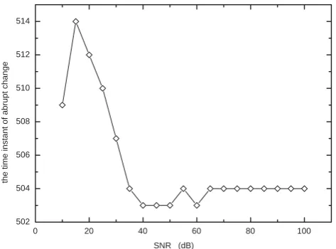
In the model time series IS3, the first 500 data have been created by the variablex in the classical Lorenz model, and the second 500 data have been created by the variablex1in the coupling model (Eq. 2). The coupling strength E be-tween the two subsystems is 0.001 in this test. The evolution curve of the model time series IS3has been shown in Fig. 6a. Similar to IS1, We can easily find that the evolution curve of scaling exponents can be roughly divided into three differ-ent parts based on differdiffer-ent fluctuation amplitudes. Then we use variance contribution procedure to analyze scaling expo-nents in Fig. 6b and c, and find that the time-instants of abrupt change are respectivelyn=503 and 504. And then we stud-ied the effect of noise on MDFA because noise is inevitable in observational data. Figure 7 shows the MDFA results for IS1 under different Signal Noise Ratio (SNR), and we find that noise has an impact on the MDFA results, especially for strong noises, but MDFA has a perfect capability to resist the effect of noise. The MDFA results of analogous tests on noise for IS2and IS3are similar to that for IS1.
4 Conclusions
We present a new method-MDFA for detection of abrupt change in dynamic structures. The tests on different model time series indicate that this new method can be able to ef-fectively detect abrupt dynamic change. What’s more, the MDFA results are almost independent of length of subseries and have a perfect capability to resist the effect of noise. The MDFA results are observably better than that of tradition methods because detection results of traditional methods ev-idently depend on lengths of subseries analyzed. The MDFA provides a reliable approach to estimate time-instants of abrupt dynamic change and overcomes the drawback of tra-ditional ones which cannot effectively detect abrupt change in dynamic structures. Based on this, this new method must be applied in the future widely.
Acknowledgements. The authors thanks anonymous reviewers and
editors for beneficial and helpful suggestions for this manuscript. This work was jointly supported by the National Natural Sciences Foundation of China (Grant No. 40325015), the National Key pro-gram development for Basic Research (Grant No. 2006CB400503).
Edited by: J. Kurths
Reviewed by: One anonymous referee
0 20 40 60 80 100 502
504 506 508 510 512 514
the time instant of abrupt change
SNR (dB)
Fig. 7. The MDFA results of IS1under different SNR, the length of
subseries is equal to 200.
References
Alexi, M. G., Brook, E. J., and Severinghaus, J. P: Abrupt change in atmospheric methane at the MIS 5b-5a transition, Geophys. Res. Lett., 34, L20703, doi:10.1029/2007GL029799, 2007.
Alley, R. B., Marotzke, J. W., Nordhaus, D., Overpeck, J. T., Peteet, D. M., and Pielke, R. A.: Abrupt climate change, Science, 229, 2005–2010, 2003.
Broecker, W. S.: Does the trigger for abrupt climate change reside in the ocean or in the atmosphere?, Science, 300, 1519–1522, 2003.
Bunde, A., Havlin S., Kantelhardt, J. W., Penzel, T., Peter, J. H., and Voigt, K.: Correlated and uncorrelated regions in heart-rate fluctuations during sleep, Phys. Rev. Lett., 85, 3736–3739, 2000. Bunde, A., Eichner, J. F., Kantelhardt, J. W., and Havlin, S.: Long-term memory: a natural mechanism for the clustering of extreme events and anomalous residual times in climate records, Phys. Rev. Lett., 94, 048701, doi:10.1103/PhsRevLett.94.048701, 2005.
Cao, H. X.: Self-memorization equation in atmospheric motion, Sci. China Ser. B, 36, 845–855, 1993.
Cao, H. X.: Characteristics of long-term climate change in Beijing with detrended fluctuation analysis, J. Chin. Geophys., 50, 420– 424, 2007.
Chen, G. and Ueta, T.: Yet another chaotic attractor, Int. J. Bifurcat. Chaos, 9, 1465–1466, 1999.
Fraedrich, K. and Blender, R.: Scaling of atmosphere
and ocean temperature correlations in observations and
climate models, Phys. Rev. Lett., 90, 108501(1–4),
doi:10.1103/PhysRevLett.90.108501, 2003.
Ganopolski, A. and Rahmstorf, S.: Abrupt glacial climate change due to stochastic resonance, Phys. Rev. Lett., 88, 038501, doi:10.1103/PhysRevLett.88.038501, 2002.
Jan, F. E., Jan., W. K., Bunde, A., and Havlin, S.: Statistics of re-turn intervals in long-term correlated records, Phys. Rev. E, 75, 011128, doi:10.1103/PhysRevE.75.011128, 2007.
Livina, V. N., Havlin, S., and Bunde, A.: Memory in the occurrence of earthquakes, Phys. Rev. Lett., 95, 208501, doi:10.1103/PhysRevLett.95.208501, 2005.
Liu, S. D., Rong, P. P., and Chen, Q.: The hierarchical structuare of climate series, Acta. Meteo. Sin., 58, 110–114, 2000.
Lorenz, E. N.: Deterministic nonperiodic flow, J. Atmos. Sci., 20, 130–141, 1963.
Mann, H. B.: Non-parametric tests against trend, Econometrica, 13, 245–259, 1945.
Maraun, D., Rust, H. W., and Timmer, J.: Tempting long-memory: on the interpretation of DFA results, Nonlin. Processes Geophys., 11, 495–503, 2004,
http://www.nonlin-processes-geophys.net/11/495/2004/. Peng, C. K., Mietus, J., Hausdorff, J. M., Havlin, S., Stanley, H.
E., and Goldberger, A. L.: Long-range anticorrelations and non-Gaussian behavior of the heartbeat, Phys. Rev. Lett., 70, 1343– 1346, 1993.
Peng, C. K., Buldyrev, S. V., Havlin, S., Simons, M., Stanley, H. E., and Goldberger, A. L.: Mosaic organization of DNA nucleotides, Phys. Rev. E, 49, 1685–1689, 1994.
Peter, T. and Rudolf, O. W.: Power spectrum and detrended fluctu-ation analysis: applicfluctu-ation to daily temperatures, Phys. Rev. E, 62, 150–160, 2000.
Pincus, S. M.: Approximate entropy as a measure of system com-plexity, P. Natl. Acad. Sci. USA, 88, 2297–2301, 1991. Pincus, S. M.: Approximate entropy (ApEn) as a complexity
mea-sure, Chaos, 5, 110–117, 1995.
Rahmstorf, S.: Timing of abrupt climate change: a precise clock, Geophys. Res. Lett., 30, 1510, doi:10.1029/2003GL017115, 2003.
Monetti, R. A., Havlin, S., and Bunde, A.: Long-term persistence in the sea surface temperature fluctuations, Physica A, 320, 581– 589, 2003.
Thomas, J. C. and Gerald, R. N.: Abrupt climate change and extinc-tion events in earth history, Science, 240, 996–1002, 1988. Wunsch, C.: Abrupt climate change: an alternative view,
Quater-nary Res., 65, 191–203, 2006.