www.astesj.com 467
Tracking and Detecting moving weak Targets
Naima Amrouche*,1,2, Ali Khenchaf2, Daoud Berkani1
1Ecole Nationale Polytechnique d’Alger, 10 Rue Frère Oudek, Elharrach, Algérie, 16200
2Lab-STICC CNRS UMR 6285, ENSTA Bretagne, 02 Rue François Verny, Brest Cedex 09, France, 29806
A R T I C L E I N F O A B S T R A C T Article history
Received: 13 December, 2017 Accepted: 24 January, 2018 Online: 10 February, 2018
Detect and tracking of moving weak targets is a complicated dynamic state estimation problem whose difficulty is increased in case of high clutter conditions or low signal to noise ratio (SNR). In this case, the track-before-detect filter (TBDF) that uses unthresholded measurements considers as an effective method for detecting and tracking a single target under low SNR conditions. In this paper, a particle filter based track-before-detect (PF-TBD) method is proposed to address the problem of track-before-detection and tracking with unthersholded data and a binary variable of the existence of the target for two motion models. Simulation results using image measurements based on TBD scenarios are also presented to demonstrate the capability of the proposed approach.
Keywords : Target Tracking Track Before Detect Detection
Particle Filter
1. Introduction
The classical approach to target tracking is based on target measurements (position, range rate, and so forth) that are extracted by thresholding the output of a signal processing unit of a surveillance sensor [1].The primary role of thresholding is to reduce the data flow and thus simplify tracking. For a target of a certain signal-to-noise ratio (SNR), the choice of the detection threshold determines the probability of target detection and the density of false alarms. The false alarm rate, on the other hand, affects the complexity of the data association problem in the tracking system. In general, higher densities of false alarms require more sophisticated data association algorithms.
The undesirable effect of thresholding the sensor data, however, is that in restricting the data flow, it also throws away potentially useful information. For high SNR targets this loss of information is of little concern because one can achieve good probability of detection with a small false alarm rate. Recent developments of stealthy military aircraft and cruise missiles have emphasized the need to detect and track low SNR targets. For these dim (stealthy) targets, there is a considerable advantage in using the unthresholded data for simultaneous detection and track initiation [2], [3]. Depending on the type of sensor in use, the unthresholded data can be a sequence of range-Doppler maps, bearing-frequency distributions.
The concept of simultaneous detection and tracking using unthresholded data is known in literatures as track-before-detect (TBD) approach. Typically TBD is implemented as a batch algorithm using the Hough transform [4], dynamic programming [2] [3] or maximum likelihood estimation [5].
TBD algorithms based on the Hough transformation, dynamic programming or maximum likelihood methods are generally computationally intensive [6]. With recent advancement in Sequential Monte Carlo techniques, TBD algorithms implemented using PF are now computationally feasible [7] [8].
In this paper we also develop a recursive Bayesian TBD estimator; however, our formulation and implementation are based on the particle filter [7] [9]. The PF based TBD incorporates unthresholded data and a binary target existence variable into the target state estimation process. The presence and absence of target are explicitly modelled [10] [11]. This concept, allows us to calculate the probability of existence of the target directly from the filter.
The paper is organized as follows: section 2 the system dynamics and measurement model, are introduced for the TBD application. In section 3 formulates the TBD approach as a nonlinear filtering problem and describes the conceptual recursive Bayesian solution. The implementation of this solution using a particle filter is presented in section 4. In section 5 collects our simulations and results. Finally, we report our conclusions and direction for future research in section 6.
ASTESJ ISSN: 2415-6698
*Naima Amrouche, 02 rue François Verny, Tel : +332 98 34 88 00 &
Email: [email protected]
www.astesj.com
2. Formulation Problem
2.1.Dynamic Model
We assume that want to track a target moving in a 2-D plane with an unknown state vector 𝑠𝑘 at time step 𝑘. We consider the state model given by:
𝑠𝑘+1 = 𝐹𝑠𝑘+ 𝑣𝑘
Where 𝐹 is the state transition matrix, assuming constant velocity motion and coordinate turn motion respectively, 𝑘 is the discrete-time index, 𝑣𝑘 is the process noise sequence, and 𝑠𝑘 is the state vector defined as:
𝑠𝑘= [𝑥𝑘 𝑥̇𝑘 𝑦𝑘 𝑦̇𝑘 𝐼𝑘]
Here (𝑥𝑘, 𝑦𝑘), (𝑥̇𝑘, 𝑦̇𝑘) and 𝐼𝑘 denote the position, velocity, and the intensity of the target, respectively.
2.2.Transition Matrix
A target can be present or absent from the surveillance region at a discrete-time 𝑘. Target presence variable 𝐸𝑘 is modelled by a two-state Markov chain, that is 𝐸𝑘= {0,1}. Here 0 denotes the event that a target is not present, while 1 denotes the opposite. Furthermore, we assume that transitional probabilities of target “birth” 𝑃𝑏 and “death” 𝑃𝑑, defined as:
𝑃𝑏 ≜ 𝑃{𝐸𝑘 = 1|𝐸𝑘−1= 0}
𝑃𝑑≜ 𝑃{𝐸𝑘= 0|𝐸𝑘−1= 1}
Are known, the other two transitional probabilities of this Markov chain, the probability of staying alive 1 − 𝑃𝑑 and the probability of remaining absent 1 − 𝑃𝑏 respectively, are given by:
1 − 𝑃𝑑≜ 𝑃{𝐸𝑘= 1|𝐸𝑘−1= 1}
1 − 𝑃𝑏≜ 𝑃{𝐸𝑘 = 0|𝐸𝑘−1= 0}
The corresponding transition matrix for the Markov process is:
Π = [1 − 𝑃𝑃 𝑏 𝑃𝑏
𝑑 1 − 𝑃𝑑]
2.3.Sensor Model
The sensor provides a sequence of two-dimensional images (frames) of the surveillance region, each image consisting of
(𝑛 × 𝑚) resolution cells (pixels). A resolution cell corresponds to
a rectangular region of dimensions △𝑥× ∆𝑦 so that the center of each cell (𝑖, 𝑗) is defined to be at (𝑖∆𝑥× 𝑗∆𝑦) for 𝑖 = 1, … 𝑛 and
= 1, … 𝑚 .
At each resolution cell (𝑖, 𝑗) the measured intensity is denoted as 𝑧𝑘(𝑖,𝑗)and modeled as:
𝑧𝑘(𝑖,𝑗)= {ℎ𝑘 (𝑖,𝑗)
(𝑠𝑘) + 𝜔𝑘(𝑖,𝑗) 𝑖𝑓 𝑡𝑎𝑟𝑔𝑒𝑡 𝑝𝑟𝑒𝑠𝑒𝑛𝑡 𝜔𝑘(𝑖,𝑗) 𝑖𝑓 𝑡𝑎𝑟𝑔𝑒𝑡 𝑎𝑏𝑠𝑒𝑛𝑡
Where ℎ𝑘(𝑖,𝑗)(𝑠𝑘) is the target contribution to intensity level in the resolution cell (𝑖, 𝑗) and 𝜔𝑘(𝑖,𝑗) is measurement noise in the resolution cell (𝑖, 𝑗), assumed to be independent from pixel to pixel and from frame to frame. Thus for a point target of intensity 𝐼𝑘 at position(𝑥𝑘, 𝑦𝑘), the contribution to pixel(𝑖, 𝑗) is approximated as:
ℎ𝑘(𝑖,𝑗)(s𝑘) ≈ ∆𝑥∆𝑦𝐼𝑘
2𝜋Σ2 exp {−
(𝑖∆𝑥−𝑥𝑘)2+(𝑗∆𝑦−𝑦𝑘)2
2Σ2 }
Where Σ is the amount of blurring introduced by the sensor. The complete measurements recorded at time 𝑘 a 𝑛 × 𝑚 matrix denoted as:
z𝑘 = {𝑧𝑘 (𝑖,𝑗)
: 𝑖 = 1, … , 𝑛, 𝑗 = 1, … , 𝑚}
While the set of complete measurements collected up to time 𝑘 is denoted as usual: Z𝑘= {𝑧𝑖, 𝑖 = 1, … 𝑘}.
3. Bayesian Solution to TBD Filtering
The formal recursive Bayesian solution can be presented as a two-step procedure, consisting of prediction and update.
3.1.Prediction
The predicted target state can be written in terms of the target state and existence at the previous time, giving
𝑝(𝑠𝑘, 𝐸𝑘= 1|𝑍𝑘−1) = (1 −
𝑃𝑑) ∫ 𝑝(𝑠𝑘|𝑠𝑘−1, 𝐸𝑘 = 1, 𝐸𝑘−1= 1) ×
𝑝(𝑠𝑘−1, 𝐸𝑘−1 = 1|𝑍𝑘−1)𝑑𝑠𝑘−1+
𝑃𝑏∫ 𝑝𝑏(𝑠𝑘)𝑝(𝑠𝑘−1, 𝐸𝑘−1 = 0|𝑍𝑘−1)𝑑𝑠𝑘−1
The pdf 𝑝𝑏(𝑠𝑘) denotes the initial target density on its appearance.
3.2.Update
The update equation in the Bayesian framework is given by:
𝑝(𝑠𝑘, 𝐸𝑘= 1|𝑍𝑘) = 𝑝(𝑧𝑘|𝑠𝑘, 𝐸𝑘= 1)𝑝(𝑠𝑘, 𝐸𝑘 = 1|𝑍𝑘−1)
𝑝(𝑧𝑘|𝑧𝑘−1)
Where prediction density 𝑝(𝑠𝑘, 𝐸𝑘= 1|𝑍𝑘−1) is given by (11) and 𝑝(𝑧𝑘|𝑠𝑘, 𝐸𝑘) is the likelihood function given by:
𝑝(𝑧𝑘|𝑠𝑘, 𝐸𝑘) =
{
∏ ∏ 𝑝𝑆+𝑁(𝑧𝑘
(𝑖,𝑗)
|𝑠𝑘) , 𝑓𝑜𝑟 𝐸𝑘= 1 𝑚
𝑗=1 𝑛 𝑖=1
∏ ∏𝑚 𝑝𝑁(𝑧𝑘(𝑖,𝑗)) , 𝑓𝑜𝑟 𝐸𝑘= 0 𝑗=1
𝑛 𝑖=1
Here 𝑝𝑁(𝑧𝑘(𝑖,𝑗)) is the probability density function of
background noise in pixel (𝑖, 𝑗), while 𝑝𝑆+𝑁(𝑧𝑘(𝑖,𝑗)|𝑠𝑘) is the likelihood of target signal plus noise in pixel (𝑖, 𝑗),given that the target is in state 𝑠𝑘, This two probability density function can be further expressed as:
𝑝𝑆+𝑁(𝑧𝑘(𝑖,𝑗)|𝑠𝑘) = 𝒩 (𝑧𝑘(𝑖,𝑗), ℎ𝑘(𝑖,𝑗), 𝜎2)
Since the target (if present) will affect only the pixels in the vicinity of its location (𝑥𝑘, 𝑦𝑘) , the expression for 𝑝(𝑧𝑘|𝑠𝑘, 𝐸𝑘 = 1) can be approximated as follows:
𝑝(𝑧𝑘|𝑠𝑘, 𝐸𝑘= 1) ≈ ∏𝑖∈𝐶𝑖(𝑠𝑘)∏𝑗∈𝐶𝑗(𝑠𝑘)𝑝𝑆+𝑁(𝑧𝑘(𝑖,𝑗)|𝑠𝑘)∙
∏𝑖∉𝐶𝑖(𝑠𝑘)∏𝑗∉𝐶𝑗(𝑠𝑘)𝑝𝑁(𝑧𝑘(𝑖,𝑗))
Where 𝐶𝑖(𝑠𝑘) and 𝐶𝑗(𝑠𝑘) are the sets of subscripts 𝑖 and 𝑗, respectively, corresponding to pixels affected by the target.
4. A Particle Filter for Track Before Detect (PF-TBD)
The recursive Bayesian solution of the track problem described in the previous section can be implemented using a particle filter [7] [9] [12] [13]has some similarities to the MMPF [14]. In this case we introduce the augmented state vector to include the existence variable.𝑦𝑘= [s𝑘𝑇 𝐸
𝑘]𝑇. Let us denote a random measure that characterizes the posterior probability density function at 𝑘 − 1, namely 𝑝(𝑦𝑘−1|𝑍𝑘−1), by {𝑦𝑘−1𝑛 , 𝜔
𝑘−1𝑛 }𝑛=1𝑁 .As usual, 𝑁 is the number of particles, while 𝑦𝑘𝑛 consists of 𝑠
𝑘𝑛 and 𝐸𝑘𝑛.The pseudocode of a single cycle of the PF developed for the TBD problem is presented in Table 1. The next step is the prediction of particle target states; this is done, however, only for those particles that are characterized by 𝐸𝑘𝑛= 1.For remaining particles (with 𝐸𝑘𝑛= 0), the target state components are undefined. There are two possible cases here:
4.1.Newborne Particles
This group of predicted particles is characterized by the transition from 𝐸𝑘−1𝑛 = 0 to 𝐸𝑘𝑛= 1.The target state particles are uniformly drawn at time step 𝑘 based on some a priori information on the minimum and maximum possible values on the target state.
4.2.Existing Particles
This group of particles that continues to stay “alive”, with 𝐸𝑘−1𝑛 = 1 to 𝐸𝑘𝑛= 1.The state transition model in equation (1) is used to update the target state particles.
The importance weights are computed next. For this purpose we need to introduce the likelihood ratio in pixel (𝑖, 𝑗) for a target in state 𝑠𝑘𝑛, defined as:
ℓ (𝑧𝑘(𝑖,𝑗)|𝑠𝑘𝑛) ≜𝑝𝑆+𝑁(𝑧𝑘 (𝑖,𝑗)
|s𝑘𝑛)
𝑝𝑛(𝑧𝑘 (𝑖,𝑗)
)
ℓ (𝑧𝑘(𝑖,𝑗)|𝑠𝑘𝑛) = exp {−ℎ𝑘
(𝑖,𝑗)
(ℎ𝑘(𝑖,𝑗)−2𝑧𝑘(𝑖,𝑗))
2𝜎2 }
Where ℎ𝑘(𝑖,𝑗) was defined in (9). Equation (18) follows from (14), (15), and (11). The importance weights (up normalizing constant) are now given by [7]:
𝜔̃𝑘𝑛=
{∏ ∏ ℓ (𝑧𝑘
(𝑖,𝑗)
|s𝑘𝑛) 𝑗∈𝐶𝑗(𝑠𝑘𝑛)
𝑖∈𝐶𝑖(𝑠𝑘𝑛) 𝑖𝑓 𝐸𝑘
𝑛= 1
1 𝑖𝑓 𝐸𝑘𝑛= 0
[{𝑦𝑘𝑛} 𝑛=1
𝑁 ] =TBD-PF[{𝑦
𝑘−1𝑛 }𝑖=1𝑁 , 𝑧𝑘]
• Target existence transitions using the Regime Transition Algorithm given in [6]
[{𝐸𝑘𝑛} 𝑛=1
𝑁 ] =RT[{𝐸
𝑘−1𝑛 }𝑛=1𝑁 , Π]
• FOR 𝑖 = 1: 𝑁
- IF a newborn particle (𝐸𝑘−1𝑛 = 0 and 𝐸𝑘𝑛= 1) Draw 𝑠𝑘𝑛∼ 𝑞
𝑏(𝑠𝑘|𝑧𝑘)
- IF an existing particle (𝐸𝑘−1𝑛 = 1 and 𝐸 𝑘𝑛= 1) Draw 𝑠𝑘𝑛∼ 𝑞(𝑠𝑘|𝑠𝑘−1𝑛 , 𝑧𝑘)
- Evaluate importance weight using (13) • END FOR
• Calculate total weight: 𝑡 =SUM[{𝜔̃𝑘𝑛}𝑛=1𝑁 ]
• FOR 𝑛 = 1: 𝑁
- Normalize: 𝜔𝑘𝑛= 𝑡−1𝜔̃𝑘𝑛 • END FOR
• Resample using systematic resampling algorithm given in [6]
[{𝑦𝑘𝑛, −, −} 𝑛=1
𝑁 ] =RESAMPLE[{𝑦
𝑘𝑛, 𝜔𝑘𝑛}𝑛=1𝑁 ]
The PF for track-before-detect performs target detection using the estimate of the posterior probability of target existence. This estimate is computed as:
𝑃̂𝑘 =∑𝑁𝑛=1𝐸𝑘𝑛
𝑁
And satisfies 0 < 𝑃̂𝑘 < 1. Target presence is declared if 𝑃̂𝑘 is above a certain threshold value. This declaration can then trigger the initialization of a track based on the estimated target state
𝑠̂𝑘∕𝑘 =∑𝑁𝑛=1𝑠𝑘𝑛∙𝐸𝑘𝑛
∑𝑁𝑛=1𝐸𝑘𝑛
5. Simulation and Results
In the simulation we used two scenarios for target motion and random walk model is adopted for target intensity.
5.1.Scenario1
The first model is a nearly constant velocity model is used. The dynamic model [15] for the target can be described by (1).
Where 𝐹 = 𝑑𝑖𝑎𝑔[𝐹1, 𝐹1] ,𝑄 = 𝑑𝑖𝑎𝑔[𝑄1, 𝑄1, 𝑞2𝑇]
and 𝐹1= [1 𝑇
0 1], 𝑄1= 𝑞1∙ [
𝑇3⁄3 𝑇2⁄2
𝑇2⁄2 𝑇 ]
Where 𝑞1 and 𝑞2 denote the level of process noise in target motion and intensity, respectively. A sequence of 30 frames of data has been generated with the following parameters:
∆𝑥= ∆𝑦= 1,𝑛 = 𝑚 = 20,𝑇 = 1𝑠,𝜎 = 3, Σ = 0.7. The target
is absent from frame 1 to frame 5 to be introduced in frame 6 with the initial intensity 𝐼0 .The initial state is
The simulations are conducted under an initial intensity 𝐼0=
9, 13 and 25, which corresponds to an SNR of 3.18,6.71, and
12 dB, respectively, according to the calculation equation 𝑆𝑁𝑅 =
10𝑙𝑜𝑔 [𝐼𝛥𝑥𝛥𝑦/2𝜋𝛴2
𝜎 ]
2
. The target exists until frame 24 and is again absent in frames 25, 26,…, 30.
Figure 1 (a) and (b) show the measurement frame at time step 20 for 6.71dB and 12 dB peak respectively.
(a) (b)
Fig. 1. Measurements Frame (20): (a) for 6.71 dB Peak SNR, (b) for 12 dB Peak SNR for CV model.
The particle filter parameters are selected as follows: transitional probabilities 𝑃𝑏 = 𝑃𝑑= 0.05 ;initial existence probability 𝜇1= 0.05; 𝜐min= −1 𝑢𝑛𝑖𝑡/𝑠 ; 𝜐max= 1 𝑢𝑛𝑖𝑡/𝑠 ; initial intensity range from 𝐼𝑚𝑖𝑛= 𝐼0− 5 to 𝐼𝑚𝑎𝑥= 𝐼0+ 5 ; 𝑝 = 2 and number of particles 𝑁 = 2000.
In figure (2) the probability of presence is shown for a SNR of 6.71 dB. Existence probability remains very stable and above 0.97 until frame 25.Then it drop sharply in frame 26, when the target is disappear.
Fig. 2. True and Estimated Target Existence Probability for SNR=6.71 dB
Figure (3) displays the true target path against the track, produced by the filter. Note how the target trajectory deviates slightly from the straight line due to process noise. The PF-TBD tracks the target with a small positional error.
Fig. 3. True and Estimated Target Trajectory for SNR=6.71 dB
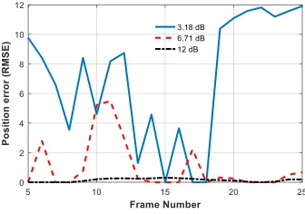
Figure (4) shows the position RMSE for three different peak SNR conditions (3.18 dB,6.71 dB, 12 dB). The position error is lower in 6.71 dB than 3.18 dB. As it can be seen, the PF-TBD was able to closely track the target even under low SNR.
Fig. 4. Position RMSE for the PF-TBD for differnet peak SNR
5.2.Scenario2
The second model is a Coordinate turn model is used [15]. The dynamic model for the target can be described by (1).
Where:
𝐹 =
[
1 𝐹1 0 𝐹2 0
0 𝐹3 0 −𝐹4 0
0 −𝐹2 1 𝐹1 0
0 𝐹4 0 𝐹3 0
0 0 0 0 1]
, 𝑄 =
[
𝑄1 𝑄2 0 𝑄3 0
𝑄2 𝑄4 −𝑄3 0 0
0 −𝑄3 𝑄1 𝑄2 0
𝑄3 0 𝑄2 𝑄4 0
0 0 0 0 𝑄5]
And 𝐹1=𝑠𝑖𝑛(Ψ𝑇)
Ψ , 𝐹2=
(−𝑐𝑜𝑠(Ψ𝑇)+1)
Ψ , 𝐹3= cos (Ψ𝑇) , 𝐹4=
sin (Ψ𝑇) , 𝑄1=2(Ψ𝑇−𝑠𝑖𝑛(Ψ𝑇))𝑞1
Ψ3 , 𝑄2=
(1−𝑐𝑜𝑠(Ψ𝑇)𝑞1)
Ψ2 𝑄3=
(Ψ𝑇−𝑠𝑖𝑛(Ψ𝑇)𝑞1)
Ψ2 , 𝑄4= 𝑞1𝑇 , 𝑄5= 𝑞2𝑇, Ψ = 6 is a constant angular
rate.
Figure 5 (a) and (b) show the measurement frame at time step 20 for 6.71dB and 12 dB peak respectively.
(a) (b)
Fig. 5. Measurements Frame (20): (a) for 6.71dB Peak SNR, (b) for 12dB Peak SNR for CT model.
In figure (6) the probability of presence is shown for a SNR of 6.71 dB. Existence probability probability is still increase above frame 7 until frame 17 and still stable until frame 25. Therefore, it drops rapidly following the target disappears from the monitoring region after frame 25.
Figure (7) shows the true and estimated target trajectories for coordinate turn model, the estimated trajectory is very close to the true trajectory.
Fig. 6. True and Estimated Target Trajectory for SNR=6.71 dB
Fig. 7. True and Estimated Target CT Trajectory for SNR=6.71
Fig. 8. Position RMSE for the PF-TBD for differnet peak SNR
6. Conclusion
In this paper, to manipulate moving weak targets, the PF-TBD algorithm is proposed for two dynamics models (CV and CT). The major advantage of the track-before-detect approach based on target existence variable and as a result, the developed particle filter can detect and track low SNR maneuvering target. The results from the simulation show that the PF-TBD algorithm has a successfully detection and tracking performance, both for constant velocity and coordinate turn models of moving targets, under severe conditions such as high noise or low SNR. Therefore, further work will mainly concentrate on how to detect and track multiple targets in high noise and high clutter.
References
[1] S. Blackman and R. Popoli, Design and Analysis of Modern Tracking System, Norwood: MA: Artech House, 1999.
[2] Y. Barniv, Dynamic programming algorithm for detecting dim moving targets, in Multitarget Multisensor Tracking: Advanced Application (Y, Bar Shalom, ed),ch 4, Norwood: MA, Artech House, 1990.
[3] J. Arnold, S. Shaw and H. Pasternack, “Efficient target tracking using dynamic programming,” IEEE Trans Aerospace and Electronic Systems,
vol. 29, pp. 44-56, January 1993.
[4] B. Carlson, E. D. Evans and S. L. Wilson, “Search radar detection and track with the Hough transform, part I: System concept,” IEEE Trans Aerospace and Electronic System, vol. 30, pp. 102-108.
[5] M. Tonissen and Y. Bar-Shalom, “Maximum likelihood track-before-detect with fluctuating target amplitude,” IEEE Trans, Aerospace and Electronic Systems, vol. 34, pp. 796-809, July 1998.
[6] R. Ristic, S. Arulampalam and N. Gordon, Beyond the Kalman Filter: Particle Filters for Tracking Applications, Boston: MA:Artech House, 2004.
[7] D. Salmond and H. Birth, “A particle filter for track-before-detect,” in Proc, Americain Control Conf, pp. 3755-3760, June 2001.
[8] Y. Boyers and H. Drissen, “Particle filter based detection for tracking,” In Proceedings of the American Control Conference,, pp. 4393-4397, June 2001.
[9] M. Rollason and D. Salmond, “A particle filter for track-before-detect of a target with unknown amplitude,” in IEE Int, Seminar Target Tracking: Algorithms and Application, p. 14, October 2001.
[10] D. B. Colegrove, A. W. Davis and J. K. Alyliffe, “Track initiation and nearest neihbours incorporated into probabilistic data association,”
Journal of Electrical and Engineers, vol. 6, pp. 191-198, September 1986.
[11] D. Musicki, R. Evans and S. Stankovic, “Integrated probabilistic data association,” IEEE Trans. Automatic Control, vol. 39, pp. 1237-1240, June 1994.
[12] D. J. Ballantyne, H. Y. Chan and M. A. Kouritzin, “A Novel branching particle method for tracking,” in Proc, SPIE, Signal and Data Processing of Small Targets,, vol. 4048, p. 287, 2000.
[13] M. G. Rutten, B. Ristic and N. J. Gordon, “A Comparison of Particle Filters for Recursive Track-before-detect,” in 7th International Conferenceon Information Fusion (FUSION), 2005.
[14] S. Mcginnity and G. W. Irwin, “Multiple Bootstrap Filter for Maneuvering Target Tracking,” IEEE Transaction of Aerospace and Electronic systems,
vol. 36, no. 3, July 2000.
[15] Y. Bar-Shalom, X. R. Li and T. Kirubarajan, Estimation with Applications to Tracking and Navigation, New York: Jhone Wiley&Sons, 2001.
[16] E. S. P and -S. A. P, “Generalized Recursive Track-Before-Detect With Proposal Partitioning for Tracking Varying Number of Multiple Targets in Low SNR,” IEEE Transactions on signal processing, vol. 64, no. 11, 2016.
[17] E. P. S and -S. P. A, “Generalized Recursive Track-Before-Detect With Proposal Partitioning for Tracking Varying Number of Multiple Targets in Low SNR,” IEEE Transactions on signal processing, vol. 64, no. 11, 2016.