Euclidean Embedding of Co-occurrence Data

Euclidean Embedding of Co-occurrence Data

Amir Globerson∗ [email protected]

Computer Science and Artificial Intelligence Laboratory Massachusetts Institute of Technology

Cambridge, MA 02139

Gal Chechik∗ [email protected]

Department of Computer Science Stanford University

Stanford CA, 94306

Fernando Pereira [email protected]

Department of Computer and Information Science University of Pennsylvania

Philadelphia PA, 19104

Naftali Tishby [email protected]

School of Computer Science and Engineering and The Interdisciplinary Center for Neural Computation The Hebrew University of Jerusalem

Givat Ram, Jerusalem 91904, Israel

Editor: John Lafferty

Abstract

Embedding algorithms search for a low dimensional continuous representation of data, but most algorithms only handle objects of a single type for which pairwise distances are specified. This paper describes a method for embedding objects of different types, such as images and text, into a single common Euclidean space, based on their co-occurrence statistics. The joint distributions are modeled as exponentials of Euclidean distances in the low-dimensional embedding space, which links the problem to convex optimization over positive semidefinite matrices. The local structure of the embedding corresponds to the statistical correlations via random walks in the Euclidean space. We quantify the performance of our method on two text data sets, and show that it consistently and significantly outperforms standard methods of statistical correspondence modeling, such as multidimensional scaling, IsoMap and correspondence analysis.

Keywords: embedding algorithms, manifold learning, exponential families, multidimensional scaling, matrix factorization, semidefinite programming

1. Introduction

Embeddings of objects in a low-dimensional space are an important tool in unsupervised learning and in preprocessing data for supervised learning algorithms. They are especially valuable for exploratory data analysis and visualization by providing easily interpretable representations of the

relationships among objects. Most current embedding techniques build low dimensional mappings that preserve certain relationships among objects. The methods differ in the relationships they choose to preserve, which range from pairwise distances in multidimensional scaling (MDS) (Cox and Cox, 1984) to neighborhood structure in locally linear embedding (Roweis and Saul, 2000) and geodesic structure in IsoMap (Tenenbaum et al., 2000). All these methods operate on objects of a single type endowed with a measure of similarity or dissimilarity.

However, embedding should not be confined to objects of a single type. Instead, it may involve different types of objects provided that those types share semantic attributes. For instance, images and words are syntactically very different, but they can be associated through their meanings. A joint embedding of different object types could therefore be useful when instances are mapped based on their semantic similarity. Once a joint embedding is achieved, it also naturally defines a measure of similarity between objects of the same type. For instance, joint embedding of images and words induces a distance measure between images that captures their semantic similarity.

Heterogeneous objects with a common similarity measure arise in many fields. For example, modern Web pages contain varied data types including text, diagrams and images, and links to other complex objects and multimedia. The objects of different types on a given page have often related meanings, which is the reason they can be found together in the first place. In biology, genes and their protein products are often characterized at multiple levels including mRNA expression levels, structural protein domains, phylogenetic profiles and cellular location. All these can often be related through common functional processes. These processes could be localized to a specific cellular compartment, activate a given subset of genes, or use a subset of protein domains. In this case the specific biological process provides a common “meaning” for several different types of data.

A key difficulty in constructing joint embeddings of heterogeneous objects is to obtain a good similarity measure. Embedding algorithms often use Euclidean distances in some feature space as a measure of similarity. However, with heterogeneous object types, objects of different types may have very different representations (such as categorical variables for some and continuous vectors for others), making this approach infeasible.

The current paper addresses these problems by using object co-occurrence statistics as a source of information about similarity. We name our method Co-occurrence Data Embedding, or CODE. The key idea is that objects which co-occur frequently are likely to have related semantics. For ex-ample, images of dogs are likely to be found in pages that contain words like_{dog, canine, bark_}, reflecting a common underlying semantic class. Co-occurrence data may be related to the geom-etry of an underlying map in several ways. First, one can simply regard co-occurrence rates as approximating pairwise distances, since rates are non-negative and can be used as input to standard metric-based embedding algorithms. However, since co-occurrence rates do not satisfy metric con-straints, interpreting them as distances is quite unnatural, leading to relatively poor results as shown in our experiments.

into products of probabilities, supporting a generative interpretation of the model as a random walk in the low-dimensional space.

Given empirical co-occurrence counts, we seek embeddings that maximize the likelihood of the observed data. The log-likelihood in this case is a non-concave function, and we describe and evaluate two approaches for maximizing it. One approach is to use a standard conjugate gradient ascent algorithm to find a local optimum. Another approach is to approximate the likelihood max-imization using a convex optmax-imization problem, where a convex non-linear function is minimized over the cone of semidefinite matrices. This relaxation is shown to yield similar empirical results to the gradient based method.

We apply CODE to several heterogeneous embedding problems. First, we consider joint embed-dings of two object types, namely words-documents and words-authors in data sets of documents. We next show how CODE can be extended to jointly embed more than two objects, as demonstrated by jointly embedding words, documents, and authors into a single map. We also obtain quantita-tive measures of performance by testing the degree to which the embedding captures ground-truth structures in the data. We use these measures to compare CODE to other embedding algorithms, and find that it consistently and significantly outperforms other methods.

An earlier version of this work was described by Globerson et al. (2005).

2. Problem Formulation

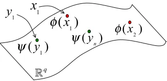
Let X and Y be two categorical variables with finite cardinalities_|X_|and_|Y_|. We observe a set of pairs_{xi,yi}ni=1 drawn IID from the joint distribution of X and Y . The sample is summarized via its empirical distribution1 _{p(x,y), which we wish to use for learning about the underlying unknown} joint distribution of X and Y . In this paper, we consider models of the unknown distribution that rely on a joint embedding of the two variables. Formally, this embedding is specified by two functions

φ: X _→Rqandψ: Y _→Rqthat map both categorical variables into the common low dimensional spaceRq, as illustrated in Figure 1.

The goal of a joint embedding is to find a geometry that reflects well the statistical relationship between the variables. To do this, we model the observed pairs as a sample from the parametric distribution p(x,y;φ,ψ), abbreviated p(x,y)when the parameters are clear from the context. Thus, our models relate the probability p(x,y)of a pair(x,y)to the embedding locationsφ(x)andψ(y).

In this work, we focus on the special case in which the model distribution depends on the squared Euclidean distance d_x2_,ybetween the embedding pointsφ(x)andψ(y):

d_x2_,y = _kφ(x)₋ψ(y)_k2₌

q

∑

k=1

(φk(x)−ψk(y))2.

Specifically, we consider models where the probability p(x,y)is proportional to e−dx2,y_{, up to} addi-tional factors described in detail below. This reflects the intuition that closer objects should co-occur more frequently than distant objects. However, a major complication of embedding models is that the embedding locationsφ(x)andψ(y)should be insensitive to the marginals p(x) =∑_yp(x,y)and

p(y) =∑_xp(x,y). To see why, consider a value x∈X with a low marginal probability p(x)1, which implies a low p(x,y)for all y. In a model where p(x,y)is proportional to e−dx2,y_{this will force}

1

( )

!

x

2

(

)

!

x

1

(

)

!

y

!

(

y

)

y

x

!q

Figure 1: Embedding of X and Y into the same q-dimensional space. The embeddings functions

φ: X_→Rqandψ: Y_→Rqdetermine the position of each instance in the low-dimensional space.

φ(x)to be far away from allψ(y). Such an embedding would reflect the marginal of x rather than its statistical relationship with all the other y values.

In what follows, we describe several methods to address this issue. Section 2.1 discusses sym-metric models, and Section 2.2 conditional ones.

2.1 Symmetric Interaction Models

The goal of joint embedding is to have the geometry in the embedded space reflect the statistical relationships between variables, rather than just their joint probability. Specifically, the locationφ(x)

should be insensitive to the marginal p(x), which just reflects the chance of observing x rather than the statistical relationship between x and different y values. To achieve this, we start by considering the ratio

rp(x,y) =

p(x,y)

p(x)p(y) , p(x) =

∑

∑

between the joint probability of x and y and the probability of observing that pair if the occurrences of x and y were independent. This ratio is widely used in statistics and information theory, for instance in the mutual information (Cover and Thomas, 1991), which is the expected value of the log of this ratio: I(X ;Y) =∑x,yp(x,y)log_pp_(x(₎x_p,y₍)_y) =∑x,yp(x,y)log rp(x,y). When X and Y are statistically independent, we have rp(x,y) =1 for all(x,y), and for any marginal distributions p(x) and p(y). Otherwise, high (low) values of rp(x,y) imply that the probability of p(x,y) is larger (smaller) than the probability assuming independent variables.

Since rp(x,y) models statistical dependency, it is a natural choice to construct a model where

rp(x,y)is proportional to e−d 2

x,y_{. A first attempt at such a model is}

p(x,y) = 1

Zp(x)p(y)e

−dx2,y , _p(_x) =

∑

p(x,y) , p(y) =

∑

p(x,y), (1)

where Z is a normalization term (partition function). The key difficulty with this model is that

p(x,y)obtained is consistent with the given marginals p(x)and p(y). This significantly complicates parameter estimation in such models, and we do not pursue them further here.2

To avoid the above difficulty, we use instead the ratio to the empirical marginals p(x)and p(y)

rp(x,y) =

p(x,y)

p(x)p(y) , p(x) =

∑

∑

This is a good approximation of rp when p(x),p(y) are close to p(x),p(y), which is a reasonable assumption for the applications that we consider. Requiring rp(x,y)to be proportional to e−d

2 x,y_{, we} obtain the following model

pMM(x,y)≡ 1

Zp(x)p(y)e −d2

x,y _{∀x∈X,∀y∈Y , (2)}

where Z =∑_x,yp(x)p(y)e−dx2,y _{is a normalization term. The subscript MM reflects the fact that} the model contains the marginal factors p(x) and p(y). We use different subscripts to distin-guish between the models that we consider (see Section 2.3). The distribution pMM(x,y)satisfies

rpMM(x,y)∝e−d 2

x,y_{, providing a direct relation between statistical dependencies and embedding} dis-tances. Note that pMM(x,y)has zero probability for any x or y that are not in the support of p(x) or p(y)(that is, p(x) =0 or p(y) =0). This does not pose a problem because such values of X or

Y will not be included in the model to begin with, since we essentially cannot learn anything about

them when variables are purely categorical. When the X or Y objects have additional structure, it may be possible to infer embeddings of unobserved values. This is discussed further in Section 9.

The model pMM(x) is symmetric with respect to the variables X and Y . The next section de-scribes a model that breaks this symmetry by conditioning on one of the variables.

2.2 Conditional Models

A standard approach to avoid modeling marginal distributions is to use conditional distributions instead of the joint distribution. In some cases, conditional models are a more plausible generating mechanism for the data. For instance, a distribution of authors and words in their works is more naturally modeled as first choosing an author according to some prior and then generating words according to the author’s vocabulary preferences. In this case, we can use the embedding distances

d_x2_,y to model the conditional word generation process rather than the joint distribution of authors and words.

The following equation defines a distance-based model for conditional co-occurrence probabil-ities:

pCM(y|x)≡ 1

Z(x)p(y)e

−d2

x,y _{∀x∈X,∀y∈Y . (3)}

Z(x) =∑_yp(y)e−dx2,y _{is a partition function for the given value x, and the subscript CM reflects the} fact that we are conditioning on X and multiplying by the marginal of Y . We can use pCM(y|x)and the empirical marginal p(x)to define a joint model pCM(x,y)≡pCM(y|x)p(x)so that

pCM(x,y) = 1

Z(x)p(x)p(y)e−

dx2,y. ₍₄₎

This model satisfies the relation rpCM(x,y)∝_Z1_(x)e−d 2

x,y _{between statistical dependency and distance.}

This implies that for a given x, the nearest neighbor ψ(y) ofφ(x) corresponds to the y with the largest dependency ratio rpCM(x,y).

A GENERATIVEPROCESS FORCONDITIONAL MODELS

One advantage of using a probabilistic model to describe complex data is that the model may reflect a mechanism for generating the data. To study such a mechanism here, we consider a simplified conditional model

pCU(y|x)≡ 1

Z(x)e

−d2 x,y₌ 1

Z(x)e

−kφ(x)−ψ(y)k2

. (5)

We also define the corresponding joint model pCU(x,y) =pCU(y|x)p(x), as in Equation 4.

The model in Equation 5 states that for a given x, the probability of generating a given y is proportional to e−d2x,y_{. To obtain a generative interpretation of this model, consider the case where} every point in the space Rq corresponds toψ(y)for some y (that is, ψis a surjective map). This will only be possible if there is a one to one mapping between the variable Y andRq, so for the purpose of this section we assume that Y is not discrete. Sampling a pair(x,y)from pCU(x,y)then corresponds to the following generative procedure:

• Sample a value of x from p(x).

• For this x, perform a random walk in the spaceRqstarting at the pointφ(x)and terminating after a fixed time T .3

• Denote the termination point of the random walk by z_∈Rq. • Return the value of y for which z=ψ(y).

The termination point of a random walk has a Gaussian distribution, with a mean given by the start-ing pointφ(x). The conditional distribution pCU(y|x)has exactly this Gaussian form, and therefore the above process generates pairs according to the distribution pCU(x,y). This process only de-scribes the generation of a single pair(xi,yi), and distinct pairs are assumed to be generated IID. It will be interesting to consider models for generating sequences of pairs via one random walk.

A generative process for the model pCM in Equation 3 is less straightforward to obtain. Intu-itively, it should correspond to a random walk that is weighted by some prior over Y . Thus, the random walk should be less likely to terminate at points ψ(y) that correspond to low p(y). The multiplicative interaction between the exponentiated distance and the prior makes it harder to define a generative process in this case.

2.3 Alternative Models

The previous sections considered several models relating distributions to embeddings. The notation we used for naming the models above is of the form pABwhere A and B specify the treatment of the

X and Y marginals, respectively. The following values are possible for A and B:

• C : The variable is conditioned on.

3. Different choices of T will correspond to different constants multiplying dx2,yin Equation 5. We assume here that T

• M : The variable is not conditioned on, and its observed marginal appears in the distribution.

• U : The variable is not conditioned on, and its observed marginal does not appear in the

distribution.

This notation can be used to define models not considered above. Some examples, which we also evaluate empirically in Section 8.5 are

pUU(x,y) ≡ 1

Ze

−d2x,y, ₍₆₎

pMC(x|y) ≡ 1

Z(y)p(x)e

−d2 x,y_,

pUC(x|y) ≡ 1

Z(y)e− d2

x,y_.

2.4 Choosing the “Right” Model

The models discussed in Sections 2.1-2.3 present different approaches to relating probabilities to distances. They differ in their treatment of marginals, and in using distances to model either joint or conditional distributions. They thus correspond to different assumptions about the data. For exam-ple, conditional models assume an asymmetric generative model, where distances are related only to conditional distributions. Symmetric models may be more appropriate when no such conditional assumption is valid. We performed a quantitative comparison of all the above models on a task of word-document embedding, as described in Section 8.5. Our results indicate that, as expected, models that address both marginals (such as pCM or pMM), and that are therefore directly related to the ratio rp(x,y), outperform models which do not address marginals. Although there are two possible conditional models, conditioning on X or on Y , for the specific task studied in Section 8.5 one of the conditional models is more sensible as a generating mechanism, and indeed yielded better results.

3. Learning the Model Parameters

We now turn to the task of learning the model parameters _{φ(x),ψ(y)_} from empirical data. In what follows, we focus on the model pCM(x,y) in Equation 4. However, all our derivations are easily applied to the other models in Section 2. Since we have a parametric model of a distribu-tion, it is natural to look for the parameters that maximize the log-likelihood of the observed pairs {(xi,yi)}ni=1. For a given set of observed pairs, the average log-likelihood is4

`(φ,ψ) =1

n

n

∑

i=1

log pCM(xi,yi).

The log-likelihood may equivalently be expressed in terms of the distribution p(x,y)since

`(φ,ψ) =

∑

p(x,y)log pCM(x,y).

4. For conditional models we can consider maximizing only the conditional log-likelihood 1_n∑n_i=1log p(yi|xi). This is

As in other cases, maximizing the log-likelihood is also equivalent to minimizing the KL divergence

DKLbetween the empirical and the model distributions, since`(φ,ψ)equals DKL[p(x,y)|pCM(x,y)] up to an additive constant.

The log-likelihood in our case is given by

`(φ,ψ) =

∑

p(x,y)log pCM(x,y)

=

∑

x,y

p(x,y)₋d2_x,y−log Z(x) +log p(x) +log p(y))

= ₋

∑

x,y

p(x,y)d2_x,y−

∑

x

p(x)log Z(x) +const, (7)

where const=∑yp(y)log p(y) +∑xp(x)log p(x) is a constant term that does not depend on the parametersφ(x)andψ(y).

Finding the optimal parameters now corresponds to solving the following optimization problem

(φ∗,ψ∗) =arg max

φ,ψ `(φ,ψ). (8)

The log-likelihood is composed of two terms. The first is (minus) the mean distance between x and

y. This will be maximized when all distances are zero. This trivial solution is avoided because of

the regularization term∑_xp(x)log Z(x), which acts to increase distances between x and y points. To characterize the maxima of the log-likelihood we differentiate it with respect to the embed-dings of individual objects(φ(x),ψ(y)), and obtain the following gradients

∂`(φ,ψ)

∂φ(x) = 2p(x)

hψ(y)_ip(y|x)− hψ(y)ipCM(y|x)

, ,

∂`(φ,ψ)

∂ψ(y) = 2pCM(y)

ψ(y)_{− h}φ(x)_ipCM(x|y)−2p(y)ψ(y)_{− h}φ(x)_ip(x|y),

where pCM(y) =∑xpCM(y|x)p(x)and pCM(x|y) = pCM_pCM(₍x_y,y₎). Equating theφ(x)gradient to zero yields:

hψ(y)_ipCM(y_|x)=hψ(y)ip(y_|x). (9)

If we fix ψ, this equation is formally similar to the one that arises in the solution of conditional maximum entropy models (Berger et al., 1996). However, there is a crucial difference in that the exponent of pCM(y|x) in conditional maximum entropy is linear in the parameters (φin our nota-tion), while in our model it also includes quadratic (norm) terms in the parameters. The effect of Equation 9 can then be described informally as that of choosingφ(x)so that the expected value of

ψunder pCM(y|x)is the same as its empirical average, that is, placing the embedding of x closer to the embeddings of those y values that have stronger statistical dependence with x.

The maximization problem of Equation 8 is not jointly convex in φ(x) andψ(y) due to the quadratic terms in d_xy2.5 To find the local maximum of the log-likelihood with respect to bothφ(x)

andψ(y)for a given embedding dimension q, we use a conjugate gradient ascent algorithm with random restarts.6 In Section 5 we describe a different approach to this optimization problem.

5. The log-likelihood is a convex function ofφ(x)for a constantψ(y), as noted in Iwata et al. (2005), but is not convex inψ(y)for a constantφ(x).

4. Relation to Other Methods

In this section we discuss other methods for representing co-occurrence data via low dimensional vectors, and study the relation between these methods and the CODE models.

4.1 Maximizing Correlations and Related Methods

Embedding the rows and columns of a contingency table into a low dimensional Euclidean space was previously studied in the statistics literature. Fisher (1940) described a method for mapping

X and Y into scalarsφ(x)andψ(y)such that the correlation coefficient betweenφ(x)andψ(y)is maximized. The method of Correspondence Analysis (CA) generalizes Fisher’s method to non-scalar mappings. More details about CA are given in Appendix A. Similar ideas have been applied to more than two variables in the Gifi system (Michailidis and de Leeuw, 1998). All these methods can be shown to be equivalent to the more widely known canonical correlation analysis (CCA) procedure (Hotelling, 1935). In CCA one is given two continuous multivariate random variables X and Y , and aims to find two sets of vectors, one for X and the other for Y , such that the correlations between the projections of the variables onto these vectors are maximized. The optimal projections for X and Y can be found by solving an eigenvalue problem. It can be shown (Hill, 1974) that if one represents X and Y via indicator vectors, the CCA of these vectors (when replicated according to their empirical frequencies) results in Fisher’s mapping and CA.

The objective of these correlation based methods is to maximize the correlation coefficient be-tween the embeddings of X and Y . We now discuss their relation to our distance-based method. First, the correlation coefficient is invariant under affine transformations and we can thus focus on centered solutions with a unity covariance matrix solutions:_hφ(X)_i=0,_hψ(Y)_i=0 and Cov(φ(X)) =

Cov(ψ(Y)) =I. In this case, the correlation coefficient is given by the following expression (we

focus on q=1 for simplicity)

ρ(φ(x),ψ(y)) =

∑

p(x,y)φ(x)ψ(y) =₋1

2

∑

x,y+1.

Maximizing the correlation is therefore equivalent to minimizing the mean distance across all pairs. This clarifies the relation between CCA and our method: Both methods aim to minimize the average distance between X and Y embeddings. However, CCA forces embeddings to be centered and scaled, whereas our method introduces a global regularization term related to the partition function. A kernel variant of CCA has been described in Lai and Fyfe (2000) and Bach and Jordan (2002), where the input vectors X and Y are first mapped to a high dimensional space, where linear projec-tion is carried out. This idea could possibly be used to obtain a kernel version of correspondence analysis, although we are not aware of existing work in that direction.

Recently, Zhong et al. (2004) presented a co-embedding approach for detecting unusual activity in video sequences. Their method also minimizes an averaged distance measure, but normalizes it by the variance of the embedding to avoid trivial solutions.

4.2 Distance-Based Embeddings

Cox, 1984, Section 7.3). These models, however, focus on specific properties of ordinal data and therefore result in optimization principles and algorithms different from our probabilistic interpre-tation.

Relating Euclidean structure to probability distributions was previously discussed by Hinton and Roweis (2003). They assume that distances between points in some X space are given, and the exponent of these distances induces a distribution p(x=i_|x= j) which is proportional to the exponent of the distance between φ(i) and φ(j). This distribution is then approximated via an exponent of distances in a low dimensional space. Our approach differs from theirs in that we treat the joint embedding of two different spaces. Therefore, we do not assume a metric structure between

X and Y , but instead use co-occurrence data to learn such a structure. The two approaches become

similar when X=Y and the empirical data exactly obeys an exponential law as in Equation 3.

Iwata et al. (2005) recently introduced the Parametric Embedding (PE) method for visualizing the output of supervised classifiers. They use the model of Equation 3 where Y is taken to be the class label, and X is the input features. Their embedding thus illustrates which X values are close to which classes, and how the different classes are inter-related. The approach presented here can be viewed as a generalization of their approach to the unsupervised case, where X and Y are arbitrary objects.

An interesting extension of locally linear embedding (Roweis and Saul, 2000) to heterogeneous embedding was presented by Ham et al. (2003). Their method essentially forces the outputs of two locally linear embeddings to be aligned such that corresponding pairs of objects are mapped to similar points.

A Bayesian network approach to joint embedding was recently studied in Mei and Shelton (2006) in the context of collaborative filtering.

4.3 Matrix Factorization Methods

The empirical joint distribution p(x,y)can be viewed as a matrix P of size|X| × |Y|. There is much literature on finding low rank approximations of matrices, and specifically matrices that represent distributions (Hofmann, 2001; Lee and Seung, 1999). Low rank approximations are often expressed as a product UVT where U and V are two matrices of size|X| ×q and|Y| ×q respectively.

In this context CODE can be viewed as a special type of low rank approximation of the matrix P. Consider the symmetric model pUUin Equation 6, and the following matrix and vector definitions:7

• LetΦbe a matrix of size_|X_{| ×}q where the ith row isφ(i). LetΨbe a matrix of size_|Y_{| ×}q

where the ithrow isψ(i).

• Define the column vector u(Φ)_∈R|X| as the set of squared Euclidean norms ofφ(i), so that

ui(φ) =kφ(i)k2. Similarly define v(ψ)∈R|Y| as vi(ψ) =kψ(i)k2.

• Denote the k-dimensional column vector of all ones by 1k.

Using these definitions, the model pUU can then be written in matrix form as

log PUU=−log Z+2ΦΨT−u(Φ)1T_|Y_|−1|X|v(Ψ)T

where the optimalΦandΨare found by minimizing the KL divergence between P and PUU.

The model for log PUU is in fact low-rank, since the rank of log PUUis at most q+2. However, note that PUU itself will not necessarily have a low rank. Thus, CODE can be viewed as a low-rank matrix factorization method, where the structure of the factorization is motivated by distances between rows ofΦandΨ, and the quality of the approximation is measured via the KL divergence. Many matrix factorization algorithms (such as Lee and Seung, 1999) use the termΦΨT above, but not the terms u(Φ) and v(Ψ). Another algorithm that uses only the ΦΨT term, but is more closely related to CODE is the sufficient dimensionality reduction (SDR) method of Globerson and Tishby (2003). SDR seeks a model

log PSDR=−log Z+ΦΨT+a1T_|Y|+1|X|bT

where a,b are vectors of dimension_|X_|,_|Y_|respectively. As in CODE, the parametersΦ,Ψ,a and b are chosen to maximize the likelihood of the observed data.

The key difference between CODE and SDR lies in the terms u(Φ)and v(Ψ)which are

non-linear inΦ andΨ. These arise from the geometric interpretation of CODE that relates distances between embeddings to probabilities. SDR does not have such an interpretation. In fact, the SDR model is invariant to the translation of either of the embedding maps (for instance, φ(x)), while fixing the other mapψ(y). Such a transformation would completely change the distances d_x2_,yand is clearly not an invariant property in the CODE models.

5. Semidefinite Representation

The CODE learning problem in Equation 8 is not jointly convex in the parametersφandψ. In this section we present a convex relaxation of the learning problem. For a sufficiently high embedding dimension this approximation is in fact exact, as we show next. For simplicity, we focus on the pCM model, although similar derivations may be applied to the other models.

5.1 The Full Rank Case

Locally optimal CODE embeddingsφ(x)andψ(y)may be found using standard unconstrained opti-mization techniques. However, the Euclidean distances used in the embedding space also allow us to reformulate the problem as constrained convex optimization over the cone of positive semidefinite (PSD) matrices (Boyd and Vandenberghe, 2004).

We begin by showing that for embeddings with dimension q=_|X_|+_|Y_|, maximizing the CODE likelihood (see Equation 8) is equivalent to minimizing a certain convex non-linear function over PSD matrices. Consider the matrix A whose columns are all the embedded vectorsφ(x)andψ(y)

A_≡[φ(1), . . . ,φ(_|X_|),ψ(1), . . . ,ψ(_|Y_|)].

Define the Gram matrix G as

G_≡ATA.

G is a matrix of the dot products between the coordinate vectors of the embedding, and is therefore

a symmetric PSD matrix of rank_≤q. Conversely, any PSD matrix of rank_≤q can be factorized as ATA, where A is some embedding matrix of dimension q. Thus we can replace optimization over

matrices A with optimization over PSD matrices of rank_≤q. Note also that the distance between

Since the log-likelihood function in Equation 7 depends only on the distances between points in X and in Y , we can write it as a function of G only.8 In what follows, we focus on the negative log-likelihood f(G) =₋`(G)

f(G) =

∑

p(x,y)(gxx+gyy−2gxy) +

∑

p(x)log

∑

p(y)e−(gxx+gyy−2gxy)_.

The likelihood maximization problem can then be written in terms of constrained minimization over the set of rank q positive semidefinite matrices9

minG f(G) s.t. G0

rank(G)_≤q.

(10)

Thus, the CODE log-likelihood maximization problem in Equation 8 is equivalent to minimizing a nonlinear objective over the set of PSD matrices of a constrained rank.

When the embedding dimension is q=_|X_|+_|Y_|the rank constraint is always satisfied and the problem reduces to

minG f(G)

s.t. G0. (11)

The minimized function f(G) consists of two convex terms: The first term is a linear function of

G; the second term is a sum of log∑exp terms of an affine expression in G. The log∑exp function is convex (Boyd and Vandenberghe, 2004, Section 4.5), and therefore the function f(G)is convex. Moreover, the set of constraints is also convex since the set of PSD matrices is a convex cone (Boyd and Vandenberghe, 2004). We conclude that when the embedding dimension is of size q=_|X_|+_|Y_|

the optimization problem of Equation 11 is convex, and thus has no local minima.

5.1.1 ALGORITHMS

The convex optimization problem in Equation 11 can be viewed as a PSD constrained geometric program.10 This is not a semidefinite program (SDP, see Vandenberghe and Boyd, 1996), since the objective function in our case is non-linear and SDPs are defined as having both a linear objective and linear constraints. As a result we cannot use standard SDP tools in the optimization. It seems like such Geometric Program/PSD problems have not been dealt with in the optimization literature, and it will be interesting to develop specialized algorithms for these cases.

The optimization problem in Equation 11 can however be solved using any general purpose con-vex optimization method. Here we use the projected gradient algorithm (Bertsekas, 1976), a simple method for constrained convex minimization. The algorithm takes small steps in the direction of the negative objective gradient, followed by a Euclidean projection on the set of PSD matrices. This projection is calculated by eliminating the contribution of all eigenvectors with negative eigenvalues to the current matrix, similarly to the PSD projection algorithm of Xing et al. (2002). Pseudo-code for this procedure is given in Figure 2.

In terms of complexity, the most time consuming part of the algorithm is the eigenvector calcu-lation which is O((_|X_|+_|Y_|)3_{)(Pan and Chen, 1999). This is reasonable when|X|+|Y|is a few} thousands but becomes infeasible for much larger values of_|X_|and_|Y_|.

8. We ignore the constant additive terms.

9. The objective f(G)is minus the log-likelihood, which is why minimization is used.

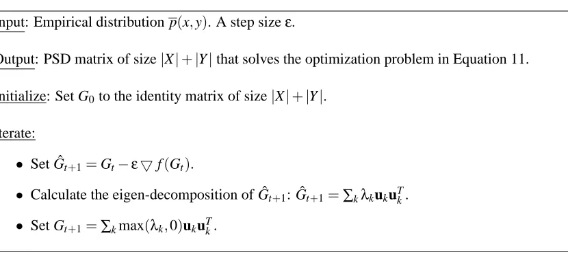
Input: Empirical distribution p(x,y). A step sizeε.

Output: PSD matrix of size_|X_|+_|Y_|that solves the optimization problem in Equation 11.

Initialize: Set G0to the identity matrix of size|X|+|Y|. Iterate:

• Set ˆGt+1=Gt−ε5f(Gt).

• Calculate the eigen-decomposition of ˆGt+1: ˆGt+1=∑kλkukuTk.

• Set Gt+1=∑kmax(λk,0)ukuT_k.

Figure 2: A projected gradient algorithm for solving the optimization problem in Equation 11. To speed up convergence we also use an Armijo rule (Bertsekas, 1976) to select the step size

εat every iteration.

5.2 The Low-Dimensional Case

Embedding into a low dimension requires constraining the rank, but this is difficult since the prob-lem in Equation 10 is not convex in the general case. One approach to obtaining low rank solutions is to optimize over a full rank G and then project it into a lower dimension via spectral decomposi-tion as in Weinberger and Saul (2006) or classical MDS. However, in the current problem, this was found to be ineffective.

A more effective approach in our case is to regularize the objective by adding a term λTr(G), for some constantλ>0. This keeps the problem convex, since the trace is a linear function of G. Furthermore, since the eigenvalues of G are non-negative, this term corresponds to`1regularization on the eigenvalues. Such regularization is likely to result in a sparse set of eigenvalues, and thus in a low dimensional solution, and is indeed a commonly used trick in obtaining such solutions (Fazel et al., 2001). This results in the following regularized problem

minG f(G) +λTr(G)

s.t. G0. (12)

Since the problem is still convex, we can again use a projected gradient algorithm as in Figure 2 for the optimization. We only need to replace∇f(Gt)withλI+∇f(Gt)where I is an identity matrix of the same size as G.

PSD-CODE

Input: A set of regularization parameters _{λi}ni=1, an embedding dimension q, and empir-ical distribution p(x,y).

Output: A q dimensional embedding of X and Y

Algorithm

• For each value ofλi:

– Use the projected gradient algorithm to solve the optimization problem in Equa-tion 12 with regularizaEqua-tion parameterλi. Denote the solution by G.

– Transform G into a rank q matrix Gq by keeping only the q eigenvectors with the largest eigenvalues.

– Calculate the likelihood of the data under the model given by the matrix Gq. Denote this likelihood by`i.

• Find theλiwhich maximizes`i, and return its corresponding embedding.

Figure 3: The PSD-CODE algorithm for finding a low dimensional embedding using PSD opti-mization.

The PSD-CODE algorithm was applied to subsets of the databases described in Section 7 and yielded similar results to those of the conjugate-gradient based algorithm. We believe that PSD algorithms may turn out to be more efficient in cases where relatively high dimensional embeddings are sought. Furthermore, with the PSD formulation it is easy to introduce additional constraints, for example on distances between subsets of points (Weinberger and Saul, 2006). Section 6.1 considers a model extension that could benefit from such a formulation.

6. Using Additional Co-occurrence Data

The methods described so far use a single co-occurrence table of two objects. However, in some cases we may have access to additional information about(X,Y)and possibly other variables. Be-low we describe extensions of CODE to these settings.

6.1 Within-Variable Similarity Measures

−12 −10 −8 −6 −4 −2 0

Log Likelihood

log(λ)

Eigenvalues

log(λ)

−10 −8 −6 −4 −2 0

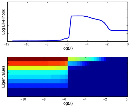
Figure 4: Results for the PSD-CODE algorithm. Data is the 5_×4 contingency table in Greenacre (1984) page 55. Top: The log-likelihood of the solution projected to two dimensions, as a function of the regularization parameterλ. Bottom: The eigenvalues of the Gram matrix obtained using the PSD algorithm for the correspondingλvalues. It can be seen that solutions with two dominant eigenvalues have higher likelihoods.

CODE map to agree with the given distances, or by adding a term which penalizes deviations from them.

Similarities between two objects in X may also be given in the form of co-occurrence data. For example, if X corresponds to words and Y corresponds to authors (see Section 7.1), we may have access to joint statistics of words, such as bigram statistics, which give additional information about which words should be mapped together. Alternatively, we may have access to data about collaboration between authors, for example, what is the probability of two authors writing a paper together. This in turn should affect the mapping of authors.

The above example can be formalized by considering two distributions p(x(1),x(2))and p(y(1),y(2))

which describe the within-type object co-occurrence rates. One can then construct a CODE model as in Equation 3 for p(x(1)|x(2))

p(x(1)_|x(2)) = p(x

(1)₎

Z(x(1)₎e−k

φ(x(1)_)−φ(x(2)_)k2 .

Denote the log-likelihood for the above model by lx(φ), and the corresponding log-likelihood for

p(y(1)_|y(2)_)by`

6.2 Embedding More than Two Variables

The notion of a common underlying semantic space is clearly not limited to two objects. For ex-ample, texts, images and audio files may all have a similar meaning and we may therefore wish to embed all three in a single space. One approach in this case could be to use joint co-occurrence statistics p(x,y,z)for all three object types, and construct a geometric-probabilistic model for the distribution p(x,y,z)using three embeddingsφ(x),ψ(y)andξ(z)(see Section 9 for further discus-sion of this approach). However, in some cases obtaining joint counts over multiple objects may not be easy. Here we describe a simple extension of CODE to the case where more than two variables are considered, but empirical distributions are available only for pairs of variables.

To illustrate the approach, consider a case with k different variables X(1), . . . ,X(k)and an addi-tional variable Y . Assume that we are given empirical joint distributions of Y with each of the X variables p(x(1),y), . . . ,p(x(k),y). It is now possible to consider a set of k CODE models p(x(i),y)for

i=1, . . . ,k,11where each X(i)will have an embeddingφ(i)(x(i))but all models will share the same

ψ(y)embedding. Given k non-negative weights w1, . . . ,wk that reflect the “relative importance” of each X(i)_{we can consider the total weighted log-likelihood of the k models given by}

`(φ(1), . . . ,φ(k),ψ) =

∑

wi

∑

p(x(i),y)log p(x(i),y).

Maximizing the above log-likelihood will effectively combine structures in all the input distributions

p(x(i),y). For example if Y =y often co-occurs with X(1)=x(1)and X(2)=x(2), likelihood will be increased by settingψ(y)to be close to bothφ(1)(x(1))andφ(2)(x(2)).

In the example above, it was assumed that only a single variable, Y , was shared between different pairwise distributions. It is straightforward to apply the same approach when more variables are shared: simply construct CODE models for all available pairwise distributions, and maximize their weighted log-likelihood.

Section 7.2 shows how this approach is used to successfully embed three different objects, namely authors, words, and documents in a database of scientific papers.

7. Applications

We demonstrate the performance of co-occurrence embedding on two real-world types of data. First, we use documents from NIPS conferences to obtain documents-word and author-word embeddings. These embeddings are used to visualize various structures in this complex corpus. We also use the multiple co-occurrence approach in Section 6.2 to embed authors, words, and documents into a single map. To provide quantitative assessment of the performance of our method, we apply it to embed the document-word 20 Usenet newsgroups data set, and we use the embedding to predict the class (newsgroup) for each document, which was not available when creating the embedding. Our method consistently outperforms previous unsupervised methods evaluated on this task.

In most of the experiments we use the conditional based model of Equation 4, except in Sec-tion 8.5 where the different models of SecSec-tion 2 are compared.

7.1 Visualizing a Document Database: The NIPS Database

Embedding algorithms are often used to visualize structures in document databases (Hinton and Roweis, 2003; Lin, 1997; Chalmers and Chitson, 1992). A common approach in these applica-tions is to obtain some measure of similarity between objects of the same type such as words, and approximate it with distances in the embedding space.

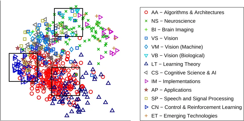
Here we used the database of all papers from the NIPS conference until 2003. The database was based on an earlier database created by Roweis (2000), that included volumes 0-12 (until 1999).12 The most recent three volumes also contain an indicator of the document’s topic, for instance, AA for Algorithms and Architectures, LT for Learning Theory, and NS for Neuroscience, as shown in Figure 5.

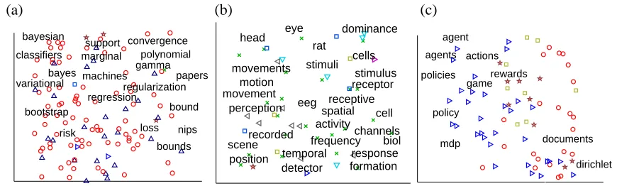
We first used CODE to embed documents and words intoR2. The results are shown in Figures 5 and 6. The empirical joint distribution was created as follows: for each document, the empirical distribution p(word_|doc)was the number of times a word appeared in the document, normalized to one; this was then multiplied by a uniform prior p(doc)to obtain p(doc,word). The CODE model we used was the conditional word-given-document model pCM(doc,word). As Figure 5 illustrates, documents with similar topics tend to be mapped next to each other (for instance, AA near LT and NS near VB), even though the topic labels were not available to the algorithm when learning the embeddings. This shows that words in documents are good indicators of the topics, and that CODE reveals these relations. Figure 6 shows the joint embedding of documents and words. It can be seen that words indeed characterize the topics of their neighboring documents, so that the joint embedding reflects the underlying structure of the data.

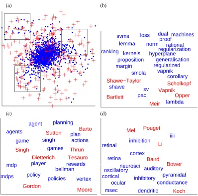
Next, we used the data to generate an authors-words matrix p(author,word) obtained from counting the frequency with which a given author uses a given word. We could now embed authors and words into R2, by using CODE to model words given authors pCM(author,word). Figure 7 demonstrates that authors are indeed mapped next to terms relevant to their work, and that authors working on similar topics are mapped to nearby points. This illustrates how co-occurrence of words and authors can be used to induce a metric on authors alone.

These examples show how CODE can be used to visualize the complex relations between doc-uments, their authors, topics and keywords.

7.2 Embedding Multiple Objects: Words, Authors and Documents

Section 6.2 presented an extension of CODE to multiple variables. Here we demonstrate that ex-tension in embedding three object types from the NIPS database: words, authors, and documents. Section 7.1 showed embeddings of(author,word) and(doc,word). However, we may also con-sider a joint embedding for the objects (author,word,doc), since there is a common semantic space underlying all three. To generate such an embedding, we apply the scheme of Section 6.2 with Y _≡word,X(1)_≡doc and X(2)_≡author. We use the two models pCM(author,word) and

pCM(doc,word), that is, two conditional models where the word variable is conditioned on the doc or on the author variables. Recall that the embedding of the words is assumed to be the same in both models. We seek an embedding of all three objects that maximizes the weighted sum of the log-likelihood of these two models.

Different strategies may be used to weight the two log-likelihoods. One approach is to assign them equal weight by normalizing each by the total number of joint assignments. This corresponds

AA − Algorithms & Architectures

NS − Neuroscience

BI − Brain Imaging

VS − Vision

VM − Vision (Machine)

VB − Vision (Biological)

LT − Learning Theory

CS − Cognitive Science & AI

IM − Implementations

AP − Applications

SP − Speech and Signal Processing

CN − Control & Reinforcement Learning

ET − Emerging Technologies

Figure 5: CODE embedding of 2483 documents and 2000 words from the NIPS database (the 2000 most frequent words, excluding the first 100, were used). Embedded documents from NIPS 15-17 are shown, with colors indicating the topic of each document. The word embeddings are not shown.

to choosing wi=_|X||1_Y(i)_|. For example, in this case the log-likelihood of pCM(author,word)will be weighted by _|word||1_author|.

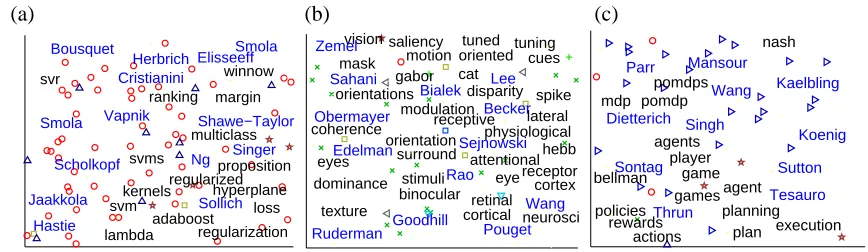
Figure 8 shows three insets of an embedding that uses the above weighting scheme.13 The insets roughly correspond to those in Figure 6. However, here we have all three objects shown on the same map. It can be seen that both authors and words that correspond to a given topic are mapped together with documents about this topic.

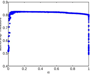
It is interesting to study the sensitivity of the result to the choice of weights wi. To evaluate this sensitivity, we introduce a quantitative measure of embedding quality: the authorship measure. The database we generated also includes the Boolean variable isauthor(doc,author) that encodes whether a given author wrote a given document. This information is not available to the CODE algorithm and can be used to evaluate the documents-authors part of the authors-words-documents embedding. Given an embedding, we find the k nearest authors to a given document and calculate what fraction of the document’s authors is in this set. We then average this across all k and all documents. Thus, for a document with three authors, this measure will be one if the three nearest authors to the document are its actual authors.

We evaluate the above authorship measure for different values of wi to study the sensitivity of the embedding quality to changing the weights. Figure 9 shows that for a very large range of wi values the measure is roughly constant, and it degrades quickly only when close to zero weight is

(a) (b) (c) bound bayesian _convergence support regression loss classifiers gamma bounds machines bayes risk polynomial nips regularization variational marginal bootstrap papers response cells cell activity frequency stimulus temporal motion position spatial stimuli receptive eye head movement channels scene movements perception recorded eeg formation detector dominance receptor rat biol policy actions agent game policies documents mdp agents rewards dirichlet

Figure 6: Each panel shows in detail one of the rectangles in Figure 5, and includes both the em-bedded documents and emem-bedded words. (a) The border region between Algorithms and Architectures (AA) and Learning Theory (LT), corresponding to the bottom rectangle in Figure 5. (b) The border region between Neuroscience NS and Biological Vision (VB), corresponding to the upper rectangle in Figure 5. (c) Control and Reinforcement Learning (CN) region (left rectangle in Figure 5).

assigned to either of the two models. The stability with respect to wi was also verified visually; embeddings were qualitatively similar for a wide range of weight values.

8. Quantitative Evaluation: The 20 Newsgroups Database

To obtain a quantitative evaluation of the effectiveness of our method, we apply it to a well controlled information retrieval task. The task contains known classes which are not used during learning, but are later used to evaluate the quality of the embedding.

8.1 The Data

We applied CODE to the widely studied 20 newsgroups corpus, consisting of 20 classes of 1000 documents each.14 This corpus was further pre-processed as described by Chechik and Tishby (2003).15 We first removed the 100 most frequent words, and then selected the next k most fre-quent words for different values of k (see below). The data was summarized as a count matrix

n(doc,word), which gives the count of each word in a document. To obtain an equal weight for all documents, we normalized the sum of each row in n(doc,word)to one, and multiplied by _|doc1 _|. The resulting matrix is a joint distribution over the document and word variables, and is denoted by

p(doc,word).

8.2 Methods Compared

Several methods were compared with respect to both homogeneous and heterogeneous embeddings of words and documents.

14. Available fromhttp://kdd.ics.uci.edu.

(a) (b) pac sv regularized shawe rational corollary proposition smola dual ranking _hyperplane generalisation svms vapnik lemma norm lambda regularization proof kernels machines margin loss Shawe−Taylor _Scholkopf Opper Meir Bartlett Vapnik (c) (d) bellman vertex player plan mdps games rewards singh agents mdp policies planning game agent actions policy Singh Thrun Moore Tesauro Barto Gordon Sutton Dietterich conductance pyramidal iiii neurosci oscillatory msec retinal ocular dendritic retina inhibition inhibitory auditory cortical cortex Koch Mel Li Baird Pouget Bower

Figure 7: CODE embedding of 2000 words and 250 authors from the NIPS database (the 250 au-thors with highest word counts were chosen; words were selected as in Figure 5). The top left panel shows embeddings for authors (red crosses) and words (blue dots). Other panels show embedded authors (only first 100 shown) and words for the areas specified by rectangles (words in blue font, authors in red). They can be seen to correspond to learning theory (b), control and reinforcement learning (c) and neuroscience (d).

• Co-Occurrence Data Embedding (CODE). Modeled the distribution of words and doc-uments using the conditional word-given-document model pCM(doc,word) of Equation 4. Models other than pCMare compared in Section 8.5.

(a) (b) (c) multiclass regularized winnow svr proposition hyperplane svms ranking regularization adaboost lambda kernels margin svm loss Singer Jaakkola Shawe−Taylor Sollich Scholkopf Vapnik Hastie Cristianini Herbrich Smola Smola Ng Bousquet Elisseeff hebb orientations mask gabor attentional eyes physiological oriented coherence binocular neurosci cat surround saliency receptor retinal cues tuned dominance modulation texture disparity lateral tuning vision stimuli receptive cortical orientation cortex eye motion spike Sejnowski Bialek Zemel Obermayer Becker Pouget Sahani Rao Wang Goodhill Lee Edelman Ruderman pomdps bellman execution plan nash rewards pomdp player games agents mdp planning policies game actions agent Singh Thrun Tesauro Sutton Dietterich Parr Wang Kaelbling Koenig Sontag Mansour

Figure 8: Embeddings of authors, words, and documents as described in Section 7.2. Words are shown in black and authors in blue (author names are capitalized). Only documents with known topics are shown. The representation of topics is as in Figure 5. We used 250 authors and 2000 words, chosen as in Figures 5 and 7. The three figures show insets of the complete embedding, which roughly correspond to the insets in Figure 6. (a) The border region between Algorithms and Architectures (AA) and Learning Theory (LT). (b) The border region between Neuroscience NS and Biological Vision (VB). (c) Control and Reinforcement Learning (CN) region.

• Singular value decomposition (SVD). Applied SVD to two count-based matrices: p(doc,word)

and log(p(doc,word) +1). Assume the SVD of a matrix P is given by P=U SVT (where S is diagonal with eigenvalues sorted in a decreasing order). Then the document embedding was taken to be U√S. Embeddings of dimension q were given by the first q columns of U√S.

An embedding for words can be obtained in a similar manner, but was not used in the current evaluation.

• Multidimensional scaling (MDS). MDS searches for an embedding of objects in a low di-mensional space, based on a predefined set of pairwise distances (Cox and Cox, 1984). One heuristic approach that is sometimes used for embedding co-occurrence data using standard MDS is to calculate distances between row vectors of the co-occurrence matrix, which is given by p(doc,word)here. This results in an embedding of the row objects (documents). Column objects (words) can be embedded similarly, but there is no straightforward way of embedding both simultaneously. Here we tested two similarity measures between row vec-tors: The Euclidean distance, and the cosine of the angle between the vectors. MDS was applied using the implementation in the MATLAB Statistical Toolbox.

• Isomap. Isomap first creates a graph by connecting each object to m of its neighbors, and then uses distances of paths in the graph for embedding using MDS. We used the MATLAB implementation provided by the Isomap authors (Tenenbaum et al., 2000), with m=10, which was the smallest value for which graphs were fully connected.

0 0.2 0.4 0.6 0.8 1 0.4

0.5 0.6 0.7 0.8 0.9

α

authorship−measure

Figure 9: Evaluation of the authors-words-documents embedding for different likelihood weights. The X axis is a numberαsuch that the weight on the pCM(doc,word)log-likelihood is

α

|word||doc| and the weight on pCM(author,word) is _|author1−α_||doc|. The valueα=0.5 results in equal weighting of the models after normalizing for size, and corresponds to the em-bedding shown in Figure 8. The Y axis is the authorship measure reflecting the quality of the joint document-author embedding.

All methods were also tested under several different normalization schemes, including TF/IDF weighting, and no document normalization. Results were consistent across all normalization schemes.

8.3 Quality Measures for Homogeneous and Heterogeneous Embeddings

Quantitative evaluation of embedding algorithms is not straightforward, since a ground-truth em-bedding is usually not well defined. Here we use the fact that documents are associated with class labels to obtain quantitative measures.

For the homogeneous embedding of the document objects, we define a measure denoted by

doc-doc, which is designed to measure how well documents with identical labels are mapped

to-gether. For each embedded document, we measure the fraction of its neighbors that are from the same newsgroup. This is repeated for all neighborhood sizes,16 and averaged over all documents and sizes, resulting in the doc-doc measure. The measure will have the value one for perfect embed-dings where same topic documents are always closer than different topic documents. For a random embedding, the measure has a value of 1/(]newsgroups).

For the heterogeneous embedding of documents and words into a joint map, we defined a mea-sure denoted by doc-word. For each document we look at its k nearest words and calculate their probability under the document’s newsgroup.17 We then average this over all neighborhood sizes of up to 100 words, and over all documents. It can be seen that the doc-word measure will be high if documents are embedded near words that are common in their class. This implies that by looking at the words close to a given document, one can infer the document’s topic. The doc-word measure

16. The maximum neighborhood size is the number of documents per topic.

could only be evaluated for CODE and CA since these are the only methods that provided joint embeddings.

8.4 Results

Figure 10 (top) illustrates the joint embedding obtained for the CODE model pCM(doc,word)when embedding documents from three different newsgroups. It can be seen that documents in different newsgroups are embedded in different regions. Furthermore, words that are indicative of a news-group topic are mapped to the region corresponding to that newsnews-group.

To obtain a quantitative estimate of homogeneous document embedding, we evaluated the

doc-doc measure for different embedding methods. Figure 11 shows the dependence of this measure

on neighborhood size and embedding dimensionality, for the different methods. It can be seen that CODE is superior to the other methods across parameter values.

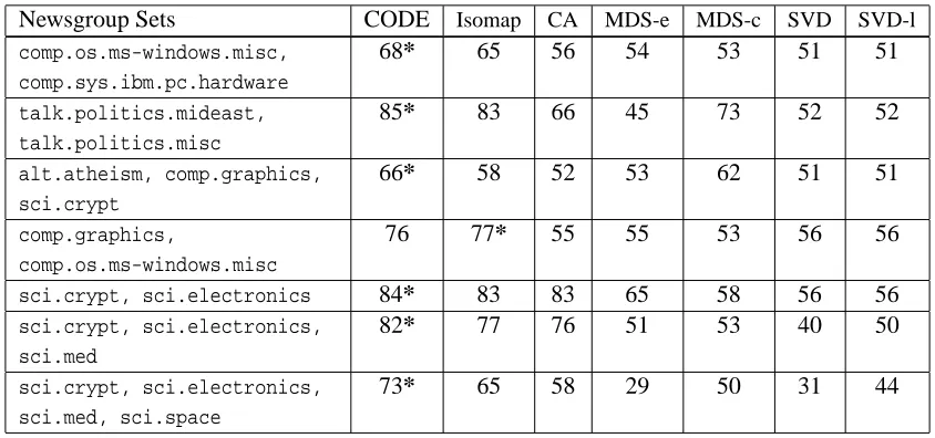
Table 1 summarizes the doc-doc measure results for all competing methods for seven different subsets.

Newsgroup Sets CODE Isomap CA MDS-e MDS-c SVD SVD-l

comp.os.ms-windows.misc, comp.sys.ibm.pc.hardware

68* 65 56 54 53 51 51

talk.politics.mideast, talk.politics.misc

85* 83 66 45 73 52 52

alt.atheism, comp.graphics,

sci.crypt

66* 58 52 53 62 51 51

comp.graphics,

comp.os.ms-windows.misc

76 77* 55 55 53 56 56

sci.crypt, sci.electronics 84* 83 83 65 58 56 56

sci.crypt, sci.electronics, sci.med

82* 77 76 51 53 40 50

sci.crypt, sci.electronics, sci.med, sci.space

73* 65 58 29 50 31 44

Table 1: doc-doc measure values (times 100) for embedding of seven newsgroups subsets. Average over neighborhood sizes 1, . . . ,1000. Embedding dimension is q=2. “MDS-e” stands for Euclidean distance, “MDS-c” for cosine distance, “SVD-l” preprocesses the data with log(count+1). The best method for each set is marked with an asterisk (*).

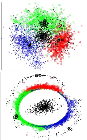
Figure 10: Visualization of two dimensional embeddings of the 20 newsgroups data under two different models. Three newsgroups are embedded: sci.crypt (red squares),

sci.electronics (green circles) and sci.med (blue xs). Top: The embed-ding of documents and words using the conditional word-given-document model

(a) (b)

2 3 4 6 8 10

0.5 0.6 0.7 0.8 0.9 1

dimension

doc−doc measure

CODE IsoMap CA MDS SVD (log)

1 10 100 1000 0.5

0.6 0.7 0.8 0.9 1

N nearest neighbors

doc−doc measure

CODE IsoMap CA MDS SVD (log)

Figure 11: Parametric dependence of the doc-doc measure for different algorithms. Embeddings were obtained for the three newsgroups described in Figure 10. (a) doc-doc as a function of embedding dimensions. Average over neighborhood sizes 1, . . . ,100. (b) doc-doc as a function of neighborhood size. Embedding dimension is q=2

The performance of the heterogeneous embedding of words and documents was evaluated using the doc-word measure for the CA and CODE algorithms. Results for seven newsgroups are shown in Figure 12b, and CODE is seen to significantly outperform CA.

Finally, we compared the performance of the gradient optimization algorithm to the PSD-CODE method described in Section 5. Here we used a smaller data set because the number of the param-eters in the PSD algorithm is quadratic in _|X_|+_|Y_|. Results for both the doc-doc and doc-word measures are shown in Figure 13, illustrating the effectiveness of the PSD algorithm, whose perfor-mance is similar the to non-convex gradient optimization scheme, and is sometimes even better.

8.5 Comparison Between Different Distribution Models

Section 2 introduced a class of possible probabilistic models for heterogeneous embedding. Here we compare the performance of these models on the 20 Newsgroup data set.

Figure 10 shows an embedding for the conditional model pCM in Equation 3 and for the sym-metric model pMM. It can be seen that both models achieve a good embedding of both the relation between documents (different classes mapped to different regions) and document-word relation (words mapped near documents with relevant subjects). However, the pMM model tends to map the documents to a circle. This can be explained by the fact that it also partially models the marginal distribution of documents, which is uniform in this case.

A more quantitative evaluation is shown in Figure 14. The figure compares various CODE mod-els with respect to the doc-doc and doc-word measures. While all modmod-els perform similarly on the

(a) (b)

CODE IsoM CA MDS SVD

0 0.2 0.4 0.6 0.8 1

doc−doc measure, mean over sets

0 0.2 0.4 0.6 0.8 1

Newsgroup sets

doc−word measure

CODE CA

Figure 12: (a) Normalized doc-doc measure (see text) averaged over 7 newsgroup sets. Embedding dimension is q=2. Sets are detailed in Table 1. Normalized doc-doc measure was calculated by rescaling at each data set, such that the poorest algorithm has score 0 and the best a score of 1. b The doc-word measure for the CODE and CA algorithms for the seven newsgroup sets. Embedding dimension is q=2.

(a) (b)

0 0.1 0.2 0.3 0.4 0.5 0.6 0.7 0.8

Newgroup Sets

doc−doc measure

GRAD PSD CA

0 0.1 0.2 0.3 0.4 0.5 0.6 0.7 0.8

Newgroup Sets

doc−word measure

GRAD PSD CA

Figure 13: Comparison of the PSD-CODE algorithm with a gradient based maximization of the CODE likelihood (denoted by GRAD) and the correspondence analysis (CA) method. Both CODE methods used the pCM(doc,word)model. Results for q=2 are shown for five newsgroup pairs (given by rows 1,2,4,5 in Table 1). Here 500 words were chosen, and 250 documents taken from each newsgroup. a. The doc-doc measure. b. The