Proximal Methods for Hierarchical Sparse Coding

Proximal Methods for Hierarchical Sparse Coding

Rodolphe Jenatton∗† [email protected]

Julien Mairal∗† [email protected]

Guillaume Obozinski† [email protected]

Francis Bach† [email protected]

INRIA - WILLOW Project-Team

Laboratoire d’Informatique de l’Ecole Normale Sup´erieure (INRIA/ENS/CNRS UMR 8548) 23, avenue d’Italie

75214 Paris CEDEX 13, France

Editor: Tong Zhang

Abstract

Sparse coding consists in representing signals as sparse linear combinations of atoms selected from a dictionary. We consider an extension of this framework where the atoms are further assumed to be embedded in a tree. This is achieved using a recently introduced tree-structured sparse regu-larization norm, which has proven useful in several applications. This norm leads to regularized problems that are difficult to optimize, and in this paper, we propose efficient algorithms for solving them. More precisely, we show that the proximal operator associated with this norm is computable exactly via a dual approach that can be viewed as the composition of elementary proximal opera-tors. Our procedure has a complexity linear, or close to linear, in the number of atoms, and allows the use of accelerated gradient techniques to solve the tree-structured sparse approximation prob-lem at the same computational cost as traditional ones using theℓ1-norm. Our method is efficient and scales gracefully to millions of variables, which we illustrate in two types of applications: first, we consider fixed hierarchical dictionaries of wavelets to denoise natural images. Then, we apply our optimization tools in the context of dictionary learning, where learned dictionary ele-ments naturally self-organize in a prespecified arborescent structure, leading to better performance in reconstruction of natural image patches. When applied to text documents, our method learns hierarchies of topics, thus providing a competitive alternative to probabilistic topic models.

Keywords: Proximal methods, dictionary learning, structured sparsity, matrix factorization

1. Introduction

Modeling signals as sparse linear combinations of atoms selected from a dictionary has become a popular paradigm in many fields, including signal processing, statistics, and machine learning. This line of research, also known as sparse coding, has witnessed the development of several well-founded theoretical frameworks (Tibshirani, 1996; Chen et al., 1998; Mallat, 1999; Tropp, 2004, 2006; Wainwright, 2009; Bickel et al., 2009) and the emergence of many efficient algorithmic tools

∗. These authors contributed equally.

(Efron et al., 2004; Nesterov, 2007; Beck and Teboulle, 2009; Wright et al., 2009; Needell and Tropp, 2009; Yuan et al., 2010).

In many applied settings, the structure of the problem at hand, such as, for example, the spatial arrangement of the pixels in an image, or the presence of variables corresponding to several levels of a given factor, induces relationships between dictionary elements. It is appealing to use this a priori knowledge about the problem directly to constrain the possible sparsity patterns. For instance, when the dictionary elements are partitioned into predefined groups corresponding to different types of features, one can enforce a similar block structure in the sparsity pattern—that is, allow only that either all elements of a group are part of the signal decomposition or that all are dismissed simultaneously (see Yuan and Lin, 2006; Stojnic et al., 2009).

This example can be viewed as a particular instance of structured sparsity, which has been lately the focus of a large amount of research (Baraniuk et al., 2010; Zhao et al., 2009; Huang et al., 2009; Jacob et al., 2009; Jenatton et al., 2009; Micchelli et al., 2010). In this paper, we concentrate on a specific form of structured sparsity, which we call hierarchical sparse coding: the dictionary elements are assumed to be embedded in a directed tree

T

, and the sparsity patterns are constrained to form a connected and rooted subtree of

T

(Donoho, 1997; Baraniuk, 1999; Baraniuk et al., 2002, 2010; Zhao et al., 2009; Huang et al., 2009). This setting extends more generally to a forest of directed trees.1

In fact, such a hierarchical structure arises in many applications. Wavelet decompositions lend themselves well to this tree organization because of their multiscale structure, and benefit from it for image compression and denoising (Shapiro, 1993; Crouse et al., 1998; Baraniuk, 1999; Baraniuk et al., 2002, 2010; He and Carin, 2009; Zhao et al., 2009; Huang et al., 2009). In the same vein, edge filters of natural image patches can be represented in an arborescent fashion (Zoran and Weiss, 2009). Imposing these sparsity patterns has further proven useful in the context of hierarchical variable selection, for example, when applied to kernel methods (Bach, 2008), to log-linear models for the selection of potential orders (Schmidt and Murphy, 2010), and to bioinformatics, to exploit the tree structure of gene networks for multi-task regression (Kim and Xing, 2010). Hierarchies of latent variables, typically used in neural networks and deep learning architectures (see Bengio, 2009, and references therein) have also emerged as a natural structure in several applications, notably to model text documents. In particular, in the context of topic models (Blei et al., 2003), a hierarchical model of latent variables based on Bayesian non-parametric methods has been proposed by Blei et al. (2010) to model hierarchies of topics.

To perform hierarchical sparse coding, our work builds upon the approach of Zhao et al. (2009) who first introduced a sparsity-inducing norm Ω leading to this type of tree-structured sparsity pattern. We tackle the resulting nonsmooth convex optimization problem with proximal methods (e.g., Nesterov, 2007; Beck and Teboulle, 2009; Wright et al., 2009; Combettes and Pesquet, 2010) and we show in this paper that its key step, the computation of the proximal operator, can be solved exactly with a complexity linear, or close to linear, in the number of dictionary elements— that is, with the same complexity as for classical ℓ1-sparse decomposition problems (Tibshirani, 1996; Chen et al., 1998). Concretely, given an m-dimensional signal x along with a dictionary

D= [d1, . . . ,dp]_∈Rm×pcomposed of p atoms, the optimization problem at the core of our paper

can be written as

min α∈Rp

1

2kx−Dαk 2

2+λΩ(α), withλ≥0.

In this formulation, the sparsity-inducing normΩencodes a hierarchical structure among the atoms of D, where this structure is assumed to be known beforehand. The precise meaning of hierarchical structure and the definition ofΩwill be made more formal in the next sections. A particular instance of this problem—known as the proximal problem—is central to our analysis and concentrates on the case where the dictionary D is orthogonal.

In addition to a speed benchmark that evaluates the performance of our proposed approach in comparison with other convex optimization techniques, two types of applications and experiments are considered. First, we consider settings where the dictionary is fixed and given a priori, corre-sponding for instance to a basis of wavelets for the denoising of natural images. Second, we show how one can take advantage of this hierarchical sparse coding in the context of dictionary learn-ing (Olshausen and Field, 1997; Aharon et al., 2006; Mairal et al., 2010a), where the dictionary is learned to adapt to the predefined tree structure. This extension of dictionary learning is notably shown to share interesting connections with hierarchical probabilistic topic models.

To summarize, the contributions of this paper are threefold:

• We show that the proximal operator for a tree-structured sparse regularization can be com-puted exactly in a finite number of operations using a dual approach. Our approach is equiva-lent to computing a particular sequence of elementary proximal operators, and has a complex-ity linear, or close to linear, in the number of variables. Accelerated gradient methods (e.g., Nesterov, 2007; Beck and Teboulle, 2009; Combettes and Pesquet, 2010) can then be applied to solve large-scale tree-structured sparse decomposition problems at the same computational cost as traditional ones using theℓ1-norm.

• We propose to use this regularization scheme to learn dictionaries embedded in a tree, which, to the best of our knowledge, has not been done before in the context of structured sparsity.

• Our method establishes a bridge between hierarchical dictionary learning and hierarchical topic models (Blei et al., 2010), which builds upon the interpretation of topic models as multinomial PCA (Buntine, 2002), and can learn similar hierarchies of topics. This point is discussed in Sections 5.5 and 6.

Note that this paper extends a shorter version published in the proceedings of the international conference of machine learning (Jenatton et al., 2010).

1.1 Notation

Vectors are denoted by bold lower case letters and matrices by upper case ones. We define for q_≥1 theℓq-norm of a vector x inRmaskxkq

△

= (∑m

i=1|xi|q)1/q, where xidenotes the i-th coordinate of x, and_kx_k∞=△ maxi=1,...,m|xi|=limq→∞kxkq. We also define theℓ0-pseudo-norm as the number of nonzero elements in a vector:2 _kx_k0

△

=#_{i s.t. xi6=0}=limq_→0+(∑m_i=1|x_i|q). We consider the Frobenius norm of a matrix X in Rm×n: _kX_kF

△

= (∑m_i=1∑n_j=1X2_{i j})1/2_{, where X}

i j denotes the entry of X at row i and column j. Finally, for a scalar y, we denote(y)+=△max(y,0).

The rest of this paper is organized as follows: Section 2 presents related work and the prob-lem we consider. Section 3 is devoted to the algorithm we propose, and Section 4 introduces the

2. Note that it would be more proper to writekxk0

0instead ofkxk0to be consistent with the traditional notationkxkq.

dictionary learning framework and shows how it can be used with tree-structured norms. Section 5 presents several experiments demonstrating the effectiveness of our approach and Section 6 con-cludes the paper.

2. Problem Statement and Related Work

Let us consider an input signal of dimension m, typically an image described by its m pixels, which we represent by a vector x inRm. In traditional sparse coding, we seek to approximate this signal by a sparse linear combination of atoms, or dictionary elements, represented here by the columns of a matrix D= [△ d1, . . . ,dp]inRm×p. This can equivalently be expressed as x≈Dαfor some sparse vectorαinRp, that is, such that the number of nonzero coefficients_kα_k0is small compared to p. The vectorαis referred to as the code, or decomposition, of the signal x.

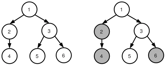
Figure 1: Example of a tree

T

when p=6. With the rule we consider for the nonzero patterns, if we haveα56=0, we must also haveαk6=0 for k in ancestors(5) ={1,3,5}.

In the rest of the paper, we focus on specific sets of nonzero coefficients—or simply, nonzero patterns—for the decomposition vector α. In particular, we assume that we are given a tree3

T

whose p nodes are indexed by j in_{1, . . . ,p_}. We want the nonzero patterns ofαto form a connected and rooted subtree of

T

; in other words, if ancestors(j)_{⊆ {}1, . . . ,p_} denotes the set of indices corresponding to the ancestors4_{of the node j in}

_T

_{(see Figure 1), the vector}α_{obeys the following} rule

αj6=0⇒[αk6=0 for all k in ancestors(j) ]. (1)

Informally, we want to exploit the structure of

T

in the following sense: the decomposition of any signal x can involve a dictionary element dj only if the ancestors of djin the tree

T

are themselves part of the decomposition.

We now review previous work that has considered the sparse approximation problem with tree-structured constraints (1). Similarly to traditional sparse coding, there are basically two lines of research, that either (A) deal with nonconvex and combinatorial formulations that are in general computationally intractable and addressed with greedy algorithms, or (B) concentrate on convex relaxations solved with convex programming methods.

2.1 Nonconvex Approaches

For a given sparsity level s≥0 (number of nonzero coefficients), the following nonconvex problem

min α∈Rp

kαk0≤s

1

2kx−Dαk 2

2 such that condition (1) is respected, (2) has been tackled by Baraniuk (1999); Baraniuk et al. (2002) in the context of wavelet approxima-tions with a greedy procedure. A penalized version of problem (2) (that addsλkαk0 to the objec-tive function in place of the constraint _kα_k0≤s) has been considered by Donoho (1997), while studying the more general problem of best approximation from dyadic partitions (see Section 6 in Donoho, 1997). Interestingly, the algorithm we introduce in Section 3 shares conceptual links with the dynamic-programming approach of Donoho (1997), which was also used by Baraniuk et al. (2010), in the sense that the same order of traversal of the tree is used in both procedures. We investigate more thoroughly the relations between our algorithm and this approach in Appendix A.

Problem (2) has been further studied for structured compressive sensing (Baraniuk et al., 2010), with a greedy algorithm that builds upon Needell and Tropp (2009). Finally, Huang et al. (2009) have proposed a formulation related to (2), with a nonconvex penalty based on an information-theoretic criterion.

2.2 Convex Approach

We now turn to a convex reformulation of the constraint (1), which is the starting point for the convex optimization tools we develop in Section 3.

2.2.1 HIERARCHICALSPARSITY-INDUCINGNORMS

Condition (1) can be equivalently expressed by its contrapositive, thus leading to an intuitive way of penalizing the vector α to obtain tree-structured nonzero patterns. More precisely, defining descendants(j)_{⊆ {}1, . . . ,p_}analogously to ancestors(j)for j in_{1, . . . ,p_}, condition (1) amounts to saying that if a dictionary element is not used in the decomposition, its descendants in the tree should not be used either. Formally, this can be formulated as:

αj=0⇒[αk=0 for all k in descendants(j) ]. (3)

From now on, we denote by

G

the set defined by

G

=△_{descendants(j); j_{∈ {}1, . . . ,p_}},and refer to each member g of

G

as a group (Figure 2). To obtain a decomposition with the desired property (3), one can naturally penalize the number of groups g in

G

that are “involved” in the decomposition of x, that is, that record at least one nonzero coefficient ofα:

∑

g_∈G

δg_{, withδ}g △ =

(

1 if there exists j_∈g such thatαj6=0,

0 otherwise. (4)

While this intuitive penalization is nonconvex (and not even continuous), a convex proxy has been introduced by Zhao et al. (2009). It was further considered by Bach (2008); Kim and Xing (2010); Schmidt and Murphy (2010) in several different contexts. For any vectorα_∈Rp, let us define

Ω(α)=△

∑

g_∈G

whereα|gis the vector of size p whose coordinates are equal to those ofαfor indices in the set g, and to 0 otherwise.5 The notation_k._kstands in practice either for theℓ2- orℓ∞-norm, and(ωg)g_∈G denotes some positive weights.6 As analyzed by Zhao et al. (2009) and Jenatton et al. (2009), when penalizing byΩ, some of the vectors α|g are set to zero for some g∈

G

.7 Therefore, the components of α corresponding to some complete subtrees of

T

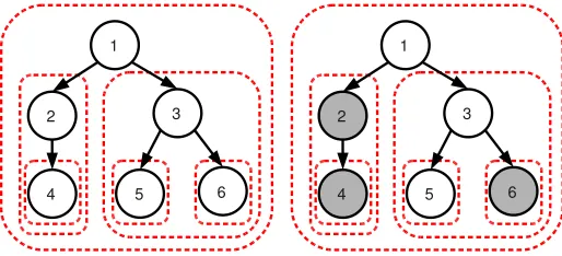
are set to zero, which exactly matches condition (3), as illustrated in Figure 2.

Figure 2: Left: example of a tree-structured set of groups

G

(dashed contours in red), corresponding to a tree

T

with p=6 nodes represented by black circles. Right: example of a sparsity pattern induced by the tree-structured norm corresponding to

G

: the groups_{2,4_},_{4_}and_{6_}are set to zero, so that the corresponding nodes (in gray) that form subtrees of

T

are removed. The remaining nonzero variables_{1,3,5_}form a rooted and connected subtree of

T

. This sparsity pattern obeys the following equivalent rules: (i) if a node is selected, the same goes for all its ancestors. (ii) if a node is not selected, then its descendant are not selected.

Note that although we presented for simplicity this hierarchical norm in the context of a single tree with a single element at each node, it can easily be extended to the case of forests of trees, and/or trees containing arbitrary numbers of dictionary elements at each node (with nodes possibly containing no dictionary element). More broadly, this formulation can be extended with the notion of tree-structured groups, which we now present:

Definition 1 (Tree-structured set of groups.)

A set of groups

G

=△_{g}g∈G is said to be tree-structured in{1, . . . ,p}, if Sg_∈Gg={1, . . . ,p}and if for all g,h_∈

G

,(g_∩h₆=/0)_⇒(g_⊆h or h_⊆g).For such a set of groups, there exists a (non-unique) total order relationsuch that:

gh _⇒ g_⊆h or g_∩h=/0 .

Given such a tree-structured set of groups

G

and its associated normΩ, we are interested throughout the paper in the following hierarchical sparse coding problem,

min

α∈Rpf(α) +λΩ(α), (5)

5. Note the difference with the notationαg, which is often used in the literature on structured sparsity, whereαgis a

vector of size|g|.

6. For a complete definition ofΩfor anyℓq-norm, a discussion of the choice of q, and a strategy for choosing the

weightsωg(see Zhao et al., 2009; Kim and Xing, 2010).

whereΩis the tree-structured norm we have previously introduced, the non-negative scalarλis a regularization parameter controlling the sparsity of the solutions of (5), and f a smooth convex loss function (see Section 3 for more details about the smoothness assumptions on f ). In the rest of the paper, we will mostly use the square loss f(α) =1

2kx−Dαk22,with a dictionary D inRm×p, but the formulation of Equation (5) extends beyond this context. In particular one can choose f to be the logistic loss, which is commonly used for classification problems (e.g., see Hastie et al., 2009).

Before turning to optimization methods for the hierarchical sparse coding problem, we consider a particular instance. The sparse group Lasso was recently considered by Sprechmann et al. (2010) and Friedman et al. (2010) as an extension of the group Lasso of Yuan and Lin (2006). To induce sparsity both groupwise and within groups, Sprechmann et al. (2010) and Friedman et al. (2010) add anℓ1 term to the regularization of the group Lasso, which given a partition

P

of{1, . . . ,p}in disjoint groups yields a regularized problem of the form

min α∈Rp

1

2kx−Dαk 2 2+λ

∑

g∈P

kα|gk2+λ′kαk1.

Since

P

is a partition, the set of groups in

P

and the singletons form together a tree-structured set of groups according to definition 1 and the algorithm we will develop is therefore applicable to this problem.

2.2.2 OPTIMIZATION FORHIERARCHICALSPARSITY-INDUCINGNORMS

While generic approaches like interior-point methods (Boyd and Vandenberghe, 2004) and subgra-dient descent schemes (Bertsekas, 1999) might be used to deal with the nonsmooth normΩ, several dedicated procedures have been proposed.

In Zhao et al. (2009), a boosting-like technique is used, with a path-following strategy in the specific case where_k._kis theℓ_∞-norm. Based on the variational equality

ku_k1=min

z∈R+p 1 2

p

∑

j=1

u2_j zj

+zj

, (6)

Kim and Xing (2010) follow a reweighted least-square scheme that is well adapted to the square loss function. To the best of our knowledge, a formulation of this type is however not available when k._k is the ℓ_∞-norm. In addition it requires an appropriate smoothing to become provably convergent. The same approach is considered by Bach (2008), but built upon an active-set strategy. Other proposed methods consist of a projected gradient descent with approximate projections onto the ball{u∈Rp;Ω(u)_≤λ_} (Schmidt and Murphy, 2010), and an augmented-Lagrangian based technique (Sprechmann et al., 2010) for solving a particular case with two-level hierarchies.

While the previously listed first-order approaches are (1) loss-function dependent, and/or (2) not guaranteed to achieve optimal convergence rates, and/or (3) not able to yield sparse solutions without a somewhat arbitrary post-processing step, we propose to resort to proximal methods8that do not suffer from any of these drawbacks.

3. Optimization

We begin with a brief introduction to proximal methods, necessary to present our contributions. From now on, we assume that f is convex and continuously differentiable with Lipschitz-continuous gradient. It is worth mentioning that there exist various proximal schemes in the literature that differ in their settings (e.g., batch versus stochastic) and/or the assumptions made on f . For instance, the material we develop in this paper could also be applied to online/stochastic frameworks (Duchi and Singer, 2009; Hu et al., 2009; Xiao, 2010) and to possibly nonsmooth functions f (e.g., Duchi and Singer, 2009; Xiao, 2010; Combettes and Pesquet, 2010, and references therein). Finally, most of the technical proofs of this section are presented in Appendix B for readability.

3.1 Proximal Operator for the NormΩ

Proximal methods have drawn increasing attention in the signal processing (e.g., Becker et al., 2009; Wright et al., 2009; Combettes and Pesquet, 2010, and numerous references therein) and the ma-chine learning communities (e.g., Bach et al., 2011, and references therein), especially because of their convergence rates (optimal for the class of first-order techniques) and their ability to deal with large nonsmooth convex problems (e.g., Nesterov, 2007; Beck and Teboulle, 2009). In a nutshell, these methods can be seen as a natural extension of gradient-based techniques when the objective function to minimize has a nonsmooth part. Proximal methods are iterative procedures. The sim-plest version of this class of methods linearizes at each iteration the function f around the current estimate ˆα, and this estimate is updated as the (unique by strong convexity) solution of the proximal problem, defined as follows:

min

α∈Rp f(αˆ) + (α−αˆ)

⊤_{∇f(αˆ) +λΩ(α) +}L

2kα−αˆk 2 2.

The quadratic term keeps the update in a neighborhood where f is close to its linear approximation, and L>0 is a parameter which is an upper bound on the Lipschitz constant of ∇f . This problem can be equivalently rewritten as:

min α∈Rp

1 2

α− αˆ −

1 L∇f(αˆ)

2 2+

λ LΩ(α).

Solving efficiently and exactly this problem is crucial to enjoy the fast convergence rates of proximal methods. In addition, when the nonsmooth termΩis not present, the previous proximal problem exactly leads to the standard gradient update rule. More generally, we define the proximal operator:

Definition 2 (Proximal Operator)

The proximal operator associated with our regularization termλΩ, which we denote by Prox_λΩ, is the function that maps a vector u_∈Rpto the unique solution of

min

v_∈Rp

1

2ku−vk 2

2+λΩ(v). (7)

• When Ω is the ℓ1-norm—that is, Ω(u) =_kuk1, the proximal operator is the well-known elementwise soft-thresholding operator,

∀j∈ {1, . . . ,p}, uj7→sign(uj)(|uj| −λ)+ =

(

0 if _|uj| ≤λ

sign(uj)(|uj| −λ) otherwise.

• WhenΩis a group-Lasso penalty withℓ2-norms—that is,Ω(u) =∑g∈Gku|gk2, with

G

being a partition of_{1, . . . ,p_}, the proximal problem is separable in every group, and the solution is a generalization of the soft-thresholding operator to groups of variables:

∀g_∈

G

,u|g7→u|g−Πk.k2≤λ[u|g] =

(

0 if _ku|gk2≤λ ku_|gk2−λ

ku_|gk2 u|g otherwise,

whereΠ_k.k2≤λdenotes the orthogonal projection onto the ball of theℓ2-norm of radiusλ.

• WhenΩis a group-Lasso penalty withℓ_∞-norms—that is,Ω(u) =∑_g∈Gku|gk∞, the solution is also a group-thresholding operator:

∀g_∈

G

, u|g7→u|g−Π_k.k1≤λ[u|g],

whereΠ_k.k1≤λ denotes the orthogonal projection onto theℓ1-ball of radiusλ, which can be solved in O(p)operations (Brucker, 1984; Maculan and Galdino de Paula, 1989). Note that when_ku|gk1≤λ, we have a group-thresholding effect, with u|g−Π_k.k1≤λ[u|g] =0.

More generally, a classical result (see, e.g., Combettes and Pesquet, 2010; Wright et al., 2009) says that the proximal operator for a norm k._k can be computed as the residual of the projection of a vector onto a ball of the dual-norm denoted by_k._k∗, and defined for any vectorκinRp by_kκ_k∗=△

max_kzk≤1z⊤κ.9 This is a classical duality result for proximal operators leading to the different closed forms we have just presented. We have indeed that Prox_λk.k2 =Id₋Π_k.k2≤λand Prox_λk.k∞=

Id−Πk.k1≤λ, where Id stands for the identity operator. Obtaining closed forms is, however, not

possible anymore as soon as some groups in

G

overlap, which is always the case in our hierarchical setting with tree-structured groups.

3.2 A Dual Formulation of the Proximal Problem

We now show that Equation (7) can be solved using a dual approach, as described in the following lemma. The result relies on conic duality (Boyd and Vandenberghe, 2004), and does not make any assumption on the choice of the norm_k._k:

Lemma 3 (Dual of the proximal problem)

Let u∈Rp_{and let us consider the problem}

max ξ∈Rp×|G|−

1 2

h

u−

∑

g∈G

ξg

2 2− kuk

2 2

i

s.t._∀g_∈

G

, _kξg_k∗≤λωgandξgj =0 if j∈/g,

(8)

whereξ= (ξg)g∈G andξgj denotes the j-th coordinate of the vectorξ g

inRp. Then, problems (7) and (8) are dual to each other and strong duality holds. In addition, the pair of primal-dual vari-ables_{v,ξ_}is optimal if and only ifξis a feasible point of the optimization problem (8), and

v=u₋∑_g∈Gξg and _∀g_∈

G

,ξg=Π_{k.k∗≤λωg}(v|g+ξg), (9) where we denote byΠ_{k.k∗≤λωg} the orthogonal projection onto the ball_{κ_∈Rp; _kκ_k∗≤λωg}. Note that we focus here on specific tree-structured groups, but the previous lemma is valid regard-less of the nature of

G

. The rationale of introducing such a dual formulation is to consider an equivalent problem to (7) that removes the issue of overlapping groups at the cost of a larger num-ber of variables. In Equation (7), one is indeed looking for a vector v of size p, whereas one is considering a matrixξinRp×|G| in Equation (8) with∑g∈G|g|nonzero entries, but with separable (convex) constraints for each of its columns.

This specific structure makes it possible to use block coordinate ascent (Bertsekas, 1999). Such a procedure is presented in Algorithm 1. It optimizes sequentially Equation (8) with respect to the variableξg, while keeping fixed the other variablesξh, for h₆=g. It is easy to see from Equation (8) that such an update of a column ξg, for a group g in

G

, amounts to computing the orthogonal projection of the vector u|g−∑h6=gξ|hgonto the ball of radiusλωgof the dual normk.k∗.

Algorithm 1 Block coordinate ascent in the dual

Inputs: u_∈Rpand set of groups

G

. Outputs: (v,ξ)(primal-dual solutions). Initialization: ξ=0.

while ( maximum number of iterations not reached ) do for g_∈

G

do

ξg

←Πk.k∗≤λωg(

u₋∑_h6=gξh

|g). end for

end while v_←u₋∑_g∈Gξg.

3.3 Convergence in One Pass

In general, Algorithm 1 is not guaranteed to solve exactly Equation (7) in a finite number of itera-tions. However, when_k._kis theℓ2- orℓ∞-norm, and provided that the groups in

G

are appropriately ordered, we now prove that only one pass of Algorithm 1, that is, only one iteration over all groups, is sufficient to obtain the exact solution of Equation (7). This result constitutes the main technical contribution of the paper and is the key for the efficiency of our procedure.

Before stating this result, we need to introduce a lemma showing that, given two nested groups g,h such that g_⊆h_{⊆ {}1, . . . ,p_}, if ξg is updated before ξh in Algorithm 1, then the optimality condition forξgis not perturbed by the update ofξh.

Lemma 4 (Projections with nested groups)

Let _k._k denote either the ℓ2- or ℓ_∞-norm, and g and h be two nested groups—that is, g _⊆h_⊆

{1, . . . ,p_}. Let u be a vector inRp, and let us consider the successive projections

ξg △

=Π_k.k∗≤tg(u|g) and ξ

h △

=Π_k.k∗≤th(u|h−ξ

g

with tg,th>0. Let us introduce v=u−ξg−ξh. The following relationships hold

ξg_=Π

k.k∗≤tg(v|g+ξ

g₎

and ξh=Π_k.k∗≤th(v|h+ξh).

The previous lemma establishes the convergence in one pass of Algorithm 1 in the case where

G

only contains two nested groups g_⊆h, provided thatξg is computed before ξh. Let us illustrate this fact more concretely. After initializing ξg and ξh to zero, Algorithm 1 first updatesξg with the formulaξg_←Π_{k.k∗≤λωg}(u|g), and then performs the following update:ξh←Π_k.k∗≤λωh(u|h−ξ

g₎

(where we have used thatξg=ξg_|h since g_⊆h). We are now in position to apply Lemma 4 which

states that the primal/dual variables_{v,ξg,ξh_}satisfy the optimality conditions (9), as described in Lemma 3. In only one pass over the groups_{g,h_}, we have in fact reached a solution of the dual formulation presented in Equation (8), and in particular, the solution of the proximal problem (7).

In the following proposition, this lemma is extended to general tree-structured sets of groups

G

:

Proposition 5 (Convergence in one pass)

Suppose that the groups in

G

are ordered according to the total order relationof Definition 1, and that the norm_k._kis either theℓ2- orℓ∞-norm. Then, after initializingξto 0, a single pass of Algorithm 1 over

G

with the orderyields the solution of the proximal problem (7).

Proof The proof largely relies on Lemma 4 and proceeds by induction. By definition of

Algo-rithm 1, the feasibility ofξis always guaranteed. We consider the following induction hypothesis

H

(h)=△

∀gh, it holds thatξg=Π_{k.k∗≤λωg}([u₋∑_g′_hξg ′

]|g+ξg) .

Since the dual variablesξare initially equal to zero, the summation over g′h, g′₆=g is equivalent to a summation over g′6=g. We initialize the induction with the first group in

G

, that, by definition of, does not contain any other group. The first step of Algorithm 1 easily shows that the induction hypothesis

H

is satisfied for this first group.

We now assume that

H

(h)is true and consider the next group h′, hh′, in order to prove that

H

(h′)is also satisfied. We have for each group g_⊆h,

ξg_=Π

k.k∗≤λωg([u−∑g′hξ

g′_]

|g+ξg) =Π_k.k∗≤λωg([u−∑g′hξ

g′_+ξg_]

|g).

Sinceξg

|h′=ξ g

for g_⊆h′, we have

[u₋∑_g′_hξg

′

]_|h′= [u−∑_g′_hξg

′

]_|h′+ξg−ξg= [u−∑_g′_hξg

′

+ξg]_|h′−ξg,

and following the update rule for the group h′,

ξh′

=Π_k.k∗≤λωh′([u−∑g′_hξg

′

]_|h′) =Π_k.k

∗≤λωh′([u−∑g′_hξg ′

+ξg]_|h′−ξg).

At this point, we can apply Lemma 4 for each group g_⊆h, which proves that the induction hy-pothesis

H

(h′) is true. Let us introduce v=△ u₋∑_g∈Gξg. We have shown that for all g in

G

, ξg_=Π

k.k∗≤λωg(v|g+ξ

g_{).As a result, the pair}

Using conic duality, we have derived a dual formulation of the proximal operator, leading to Algo-rithm 1 which is generic and works for any norm_k._k, as long as one is able to perform projections onto balls of the dual norm_k._k∗. We have further shown that when_k._kis theℓ2- or theℓ∞-norm, a single pass provides the exact solution when the groups

G

are correctly ordered. We show however in Appendix C, that, perhaps surprisingly, the conclusions of Proposition 5 do not hold for general

ℓq-norms, if q∈ {/ 1,2,∞}. Next, we give another interpretation of this result.

3.4 Interpretation in Terms of Composition of Proximal Operators

In Algorithm 1, since all the vectors ξg are initialized to 0, when the group g is considered, we have by induction u₋∑_h6=gξh=u₋∑_hgξh. Thus, to maintain at each iteration of the inner loop

v=u₋∑h₆=gξh one can instead update v after updating ξg according to v←v−ξg. Moreover, since ξg is no longer needed in the algorithm, and since only the entries of v indexed by g are updated, we can combine the two updates into v|g←v|g−Π_k.k∗≤λωg(v|g), leading to a simplified

Algorithm 2 equivalent to Algorithm 1.

Algorithm 2 Practical Computation of the Proximal Operator forℓ2- orℓ∞-norms. Inputs: u_∈Rpand an ordered tree-structured set of groups

G

.

Outputs: v (primal solution). Initialization: v=u.

for g_∈

G

, following the order, do

v|g←v|g−Π_k.k∗≤λωg(v|g). end for

Actually, in light of the classical relationship between proximal operator and projection (as discussed in Section 3.1), it is easy to show that each update v|g←v|g−Π_k.k∗≤λωg(v|g)is equivalent

to v|g←Proxλωgk.k[v|g]. To simplify the notations, we define the proximal operator for a group g in

G

as Proxg(u)=△Prox_λωgk.k(u|g)for every vector u inRp.

Thus, Algorithm 2 in fact performs a sequence of_|

G

_|proximal operators, and we have shown the following corollary of Proposition 5:

Corollary 6 (Composition of Proximal Operators)

Let g14. . .4gmsuch that

G

={g1, . . . ,gm}. The proximal operator ProxλΩ associated with the normΩcan be written as the composition of elementary operators:

Prox_λΩ=Proxgm_{◦. . .◦Prox}g1_.

3.5 Efficient Implementation and Complexity

Since Algorithm 2 involves_|

G

|projections on the dual balls (respectively theℓ2- and theℓ1-balls for theℓ2- andℓ_∞-norms) of vectors inRp, in a first approximation, its complexity is at most O(p2), because each of these projections can be computed in O(p) operations (Brucker, 1984; Maculan and Galdino de Paula, 1989). But in fact, the algorithm performs one projection for each group g involving_|g_|variables, and the total complexity is therefore O

∑g∈G|g|

Algorithm 3 Fast computation of the Proximal operator forℓ2-norm case.

Require: u_∈Rp (input vector), set of groups

G

,(ωg)g∈G (positive weights), and g0(root of the tree).

1: Variables:ρ= (ρg)g_∈G inR|G| (scaling factors); v inRp(output, primal variable).

2: computeSqNorm(g0).

3: recursiveScaling(g0,1).

4: Return v (primal solution).

ProcedurecomputeSqNorm(g)

1: Compute the squared norm of the group:ηg← kuroot(g)k22+∑h∈children(g)computeSqNorm(h).

2: Compute the scaling factor of the group:ρg← 1−λωg/√ηg

+.

3: Returnηgρ2g.

ProcedurerecursiveScaling(g,t)

1: ρ_g←tρg.

2: vroot(g)←ρguroot(g).

3: for h_∈children(g)do

4: recursiveScaling(h,ρg).

5: end for

Lemma 7 (Complexity of Algorithm 2)

Algorithm 2 gives the solution of the primal problem Equation (7) in O(pd)operations, where d is the depth of the tree.

Lemma 7 should not suggest that the complexity is linear in p, since d could depend of p as well, and in the worst case the hierarchy is a chain, yielding d= p₋1. However, in a balanced tree, d =O(log(p)). In practice, the structures we have considered experimentally are relatively flat, with a depth not exceeding d=5, and the complexity is therefore almost linear.

Moreover, in the case of theℓ2-norm, it is actually possible to propose an algorithm with com-plexity O(p). Indeed, in that case each of the proximal operators Proxg is a scaling operation:

v|g← 1−λωg/kv|gk2

+v|g. The composition of these operators in Algorithm 1 thus corresponds to performing sequences of scaling operations. The idea behind Algorithm 3 is that the correspond-ing scalcorrespond-ing factors depend only on the norms of the successive residuals of the projections and that these norms can be computed recursively in one pass through all nodes in O(p)operations; finally, computing and applying all scalings to each entry takes then again O(p)operations.

To formulate the algorithm, two new notations are used: for a group g in

G

, we denote by root(g)

the indices of the variables that are at the root of the subtree corresponding to g,10and by children(g)

the set of groups that are the children of root(g) in the tree. For example, in the tree presented in Figure 2, root(_{3,5,6}) =_{3}, root(_{1,2,3,4,5,6}) =_{1}, children(_{3,5,6}) =_{{5},_{6}}, and children(_{1,2,3,4,5,6_})=_{{2,4_},_{3,5,6_}}. Note that all the groups of children(g)are necessarily included in g. The next lemma is proved in Appendix B.

Lemma 8 (Correctness and complexity of Algorithm 3)

When_k._kis chosen to be theℓ2-norm, Algorithm 3 gives the solution of the primal problem Equa-tion (7) in O(p)operations.

So far the dictionary D was fixed to be for example a wavelet basis. In the next section, we apply the tools we developed for solving efficiently problem (5) to learn a dictionary D adapted to our hierarchical sparse coding formulation.

4. Application to Dictionary Learning

We start by briefly describing dictionary learning.

4.1 The Dictionary Learning Framework

Let us consider a set X= [x1, . . . ,xn]inRm×nof n signals of dimension m. Dictionary learning is a matrix factorization problem which aims at representing these signals as linear combinations of the dictionary elements, that are the columns of a matrix D= [d1, . . . ,dp]inRm×p. More precisely, the dictionary D is learned along with a matrix of decomposition coefficients A= [α1_{, . . . ,α}n_]inRp×n_, so that xi_≈Dαifor every signal xi.

While learning simultaneously D and A, one may want to encode specific prior knowledge about the problem at hand, such as, for example, the positivity of the decomposition (Lee and Seung, 1999), or the sparsity of A (Olshausen and Field, 1997; Aharon et al., 2006; Lee et al., 2007; Mairal et al., 2010a). This leads to penalizing or constraining(D,A)and results in the following formulation:

min

D_∈D,A_∈A 1 n

n

∑

i=1

h1

2kx i

−Dαi_k2₂+λΨ(αi)i, (10) where

A

and

D

denote two convex sets andΨis a regularization term, usually a norm or a squared norm, whose effect is controlled by the regularization parameterλ>0. Note that

D

is assumed to be bounded to avoid any degenerate solutions of Problem (10). For instance, the standard sparse coding formulation takesΨto be theℓ1-norm,

D

to be the set of matrices in Rm×pwhose columns have unitℓ2-norm, with

A

=Rp×n(Olshausen and Field, 1997; Lee et al., 2007; Mairal et al., 2010a).

However, this classical setting treats each dictionary element independently from the others, and does not exploit possible relationships between them. To embed the dictionary in a tree structure, we therefore replace theℓ1-norm by our hierarchical norm and setΨ=Ωin Equation (10).

A question of interest is whether hierarchical priors are more appropriate in supervised settings or in the matrix-factorization context in which we use it. It is not so common in the supervised setting to have strong prior information that allows us to organize the features in a hierarchy. On the contrary, in the case of dictionary learning, since the atoms are learned, one can argue that the dictionary elements learned will have to match well the hierarchical prior that is imposed by the regularization. In other words, combining structured regularization with dictionary learning has precisely the advantage that the dictionary elements will self-organize to match the prior.

4.2 Learning the Dictionary

Optimization for dictionary learning has already been intensively studied. We choose in this paper a typical alternating scheme, which optimizes in turn D and A= [α1_{, . . . ,}αn_{]while keeping the other} variable fixed (Aharon et al., 2006; Lee et al., 2007; Mairal et al., 2010a).11 Of course, the convex optimization tools we develop in this paper do not change the intrinsic non-convex nature of the

dictionary learning problem. However, they solve the underlying convex subproblems efficiently, which is crucial to yield good results in practice. In the next section, we report good performance on some applied problems, and we show empirically that our algorithm is stable and does not seem to get trapped in bad local minima. The main difficulty of our problem lies in the optimization of the vectorsαi, i in _{1, . . . ,n_}, for the dictionary D kept fixed. Because of Ω, the corresponding convex subproblem is nonsmooth and has to be solved for each of the n signals considered. The optimization of the dictionary D (for A fixed), which we discuss first, is in general easier.

4.2.1 UPDATING THEDICTIONARYD

We follow the matrix-inversion free procedure of Mairal et al. (2010a) to update the dictionary. This method consists in iterating block-coordinate descent over the columns of D. Specifically, we assume that the domain set

D

has the form

D

µ

△

=_{D_∈Rm×p,µ_kdj_k1+ (1−µ)kdjk22≤1,for all j∈ {1, . . . ,p}}, (11) or

D

+

µ

△

=

D

µ∩Rm+×p, with µ∈[0,1]. The choice for these particular domain sets is motivated

by the experiments of Section 5. For natural image patches, the dictionary elements are usually constrained to be in the unitℓ2-norm ball (i.e.,

D

=

D0

), while for topic modeling, the dictionary elements are distributions of words and therefore belong to the simplex (i.e.,

D

=

D

₁+). The update of each dictionary element amounts to performing a Euclidean projection, which can be computed efficiently (Mairal et al., 2010a). Concerning the stopping criterion, we follow the strategy from the same authors and go over the columns of D only a few times, typically 5 times in our experiments. Although we have not explored locality constraints on the dictionary elements, these have been shown to be particularly relevant to some applications such as patch-based image classification (Yu et al., 2009). Combining tree structure and locality constraints is an interesting future research.

4.2.2 UPDATING THEVECTORSαi

The procedure for updating the columns of A is based on the results derived in Section 3.3. Further-more, positivity constraints can be added on the domain of A, by noticing that for our normΩand any vector u inRp, adding these constraints when computing the proximal operator is equivalent to solving minv∈Rp 1

2k[u]+−vk22+λΩ(v).This equivalence is proved in Appendix B.6. We will indeed use positive decompositions to model text corpora in Section 5. Note that by constraining the decompositionsαi to be nonnegative, some entriesαi_j may be set to zero in addition to those already zeroed out by the normΩ. As a result, the sparsity patterns obtained in this way might not satisfy the tree-structured condition (1) anymore.

5. Experiments

We next turn to the experimental validation of our hierarchical sparse coding.

5.1 Implementation Details

(2007) and Beck and Teboulle (2009), and finally opted for the latter since, for a comparable level of precision, fewer calls of the proximal operator are required. The basic proximal scheme presented in Section 3.1 is formalized by Beck and Teboulle (2009) as an algorithm called ISTA; the same authors propose moreover an accelerated variant, FISTA, which is a similar procedure, except that the operator is not directly applied on the current estimate, but on an auxiliary sequence of points that are linear combinations of past estimates. This latter algorithm has an optimal convergence rate in the class of first-order techniques, and also allows for warm restarts, which is crucial in the alternating scheme of dictionary learning.12

Finally, we monitor the convergence of the algorithm by checking the relative decrease in the cost function.13 Unless otherwise specified, all the algorithms used in the following experiments are implemented in C/C++, with a Matlab interface. Our implementation is freely available at

http://www.di.ens.fr/willow/SPAMS/.

5.2 Speed Benchmark

To begin with, we conduct speed comparisons between our approach and other convex programming methods, in the setting whereΩis chosen to be a linear combination ofℓ2-norms. The algorithms that take part in the following benchmark are:

• Proximal methods, with ISTA and the accelerated FISTA methods (Beck and Teboulle, 2009). • A reweighted-least-square scheme (Re-ℓ2), as described by Jenatton et al. (2009); Kim and Xing (2010). This approach is adapted to the square loss, since closed-form updates can be used.14

• Subgradient descent, whose step size is taken to be equal either to a/(k+b)or a/(√k+b) (re-spectively referred to as SG and SGsqrt), where k is the iteration number, and(a,b)are the best15 parameters selected on the logarithmic grid(a,b)_{∈ {}10−4_{, . . . ,10}3_{} × {10}−2_{, . . . ,10}5_}.

• A commercial software (Mosek, available athttp://www.mosek.com/) for second-order cone programming (SOCP).

Moreover, the experiments we carry out cover various settings, with notably different sparsity regimes, that is, low, medium and high, respectively corresponding to about 50%,10% and 1% of the total number of dictionary elements. Eventually, all reported results are obtained on a single core of a 3.07Ghz CPU with 8GB of memory.

5.2.1 HIERARCHICALDICTIONARY OFNATURALIMAGEPATCHES

In this first benchmark, we consider a least-squares regression problem regularized byΩthat arises in the context of denoising of natural image patches, as further exposed in Section 5.4. In particular, based on a hierarchical dictionary, we seek to reconstruct noisy 16_×16-patches. The dictionary we use is represented on Figure 7. Although the problem involves a small number of variables, that is, p=151 dictionary elements, it has to be solved repeatedly for tens of thousands of patches, at moderate precision. It is therefore crucial to be able to solve this problem quickly and efficiently.

12. Unless otherwise specified, the initial stepsize in ISTA/FISTA is chosen as the maximum eigenvalue of the sampling covariance matrix divided by 100, while the growth factor in the line search is set to 1.5.

13. We are currently investigating algorithms for computing duality gaps based on network flow optimization tools (Mairal et al., 2010b).

14. The computation of the updates related to the variational formulation (6) also benefits from the hierarchical structure ofG, and can be performed in O(p)operations.

−3 −2 −1 0 −8 −6 −4 −2 0 2

log(CPU time in seconds)

log(relative distance to optimum)

SG SG_sqrt Fista Ista Re−L2 SOCP

(a) scale: small, regul.: low

−3 −2 −1 0

−8 −6 −4 −2 0 2

log(CPU time in seconds)

log(relative distance to optimum)

SG SG_sqrt Fista Ista Re−L2 SOCP

(b) scale: small, regul.: medium

−3 −2 −1 0

−8 −6 −4 −2 0 2

log(CPU time in seconds)

log(relative distance to optimum)

SG SG_sqrt Fista Ista Re−L2 SOCP

(c) scale: small, regul.: high

Figure 3: Benchmark for solving a least-squares regression problem regularized by the hierarchical normΩ. The experiment is small scale, m=256,p=151, and shows the performances of six opti-mization methods (see main text for details) for three levels of regularization. The curves represent the relative value of the objective to the optimal value as a function of the computational time in second on a log₁₀/log₁₀scale. All reported results are obtained by averaging 5 runs.

We can draw several conclusions from the results of the simulations reported in Figure 3. First, we observe that in most cases, the accelerated proximal scheme performs better than the other approaches. In addition, unlike FISTA, ISTA seems to suffer in non-sparse scenarios. In the least sparse setting, the reweighted-ℓ2scheme is the only method that competes with FISTA. It is however not able to yield truly sparse solutions, and would therefore need a subsequent (somewhat arbitrary) thresholding operation. As expected, the generic techniques such as SG and SOCP do not compete with dedicated algorithms.

−1 0 1 2 3 4

−5 −4 −3 −2 −1 0 1 2

log(CPU time in seconds)

log(relative distance to optimum)

SG SG_sqrt Fista Ista

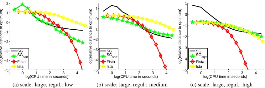
(a) scale: large, regul.: low

−1 0 1 2 3 4

−5 −4 −3 −2 −1 0 1

log(CPU time in seconds)

log(relative distance to optimum)

SG SG_sqrt Fista Ista

(b) scale: large, regul.: medium

−1 0 1 2 3 4

−5 −4 −3 −2 −1 0 1

log(CPU time in seconds)

log(relative distance to optimum)

SG SG_sqrt Fista Ista

(c) scale: large, regul.: high

5.2.2 MULTI-CLASSCLASSIFICATION OF CANCERDIAGNOSIS

The second benchmark explores a different supervised learning setting, where f is no longer the square loss function. The goal is to demonstrate that our optimization tools apply in various scenar-ios, beyond traditional sparse approximation problems. To this end, we consider a gene expression data set16 _{in the context of cancer diagnosis. More precisely, we focus on a multi-class} classifica-tion problem where the number m of samples to be classified is small compared to the number p of gene expressions that characterize these samples. Each atom thus corresponds to a gene expression across the m samples, whose class labels are recorded in the vector x inRm_.

The data set contains m=308 samples, p=30 017 variables and 26 classes. In addition, the data exhibit highly-correlated dictionary elements. Inspired by Kim and Xing (2010), we build the tree-structured set of groups

G

using Ward’s hierarchical clustering (Johnson, 1967) on the gene expressions. The norm Ω built in this way aims at capturing the hierarchical structure of gene expression networks (Kim and Xing, 2010).

Instead of the square loss function, we consider the multinomial logistic loss function that is better suited to deal with multi-class classification problems (see, e.g., Hastie et al., 2009). As a direct consequence, algorithms whose applicability crucially depends on the choice of the loss function f are removed from the benchmark. This is the case with reweighted-ℓ2schemes that do not have closed-form updates anymore. Importantly, the choice of the multinomial logistic loss function leads to an optimization problem over a matrix with dimensions p times the number of classes (i.e., a total of 30 017_×26_≈780 000 variables). Also, due to scalability issues, generic interior point solvers could not be considered here.

The results in Figure 4 highlight that the accelerated proximal scheme performs overall better that the two other methods. Again, it is important to note that both proximal algorithms yield sparse solutions, which is not the case for SG.

5.3 Denoising with Tree-Structured Wavelets

We demonstrate in this section how a tree-structured sparse regularization can improve classical wavelet representation, and how our method can be used to efficiently solve the corresponding large-scale optimization problems. We consider two wavelet orthonormal bases, Haar and Daubechies3 (see Mallat, 1999), and choose a classical quad-tree structure on the coefficients, which has notably proven to be useful for image compression problems (Baraniuk, 1999). This experiment follows the approach of Zhao et al. (2009) who used the same tree-structured regularization in the case of small one-dimensional signals, and the approach of Baraniuk et al. (2010) and Huang et al. (2009) images where images were reconstructed from compressed sensing measurements with a hierarchical nonconvex penalty.

We compare the performance for image denoising of both nonconvex and convex approaches. Specifically, we consider the following formulation

min α∈Rm

1

2kx−Dαk 2

2+λψ(α) =_αmin ∈Rm

1 2kD

⊤_x−αk2

2+λψ(α),

where D is one of the orthonormal wavelet basis mentioned above, x is the input noisy image, Dα is the estimate of the denoised image, andψis a sparsity-inducing regularization. Note that in this case, m=p. We first consider classical settings whereψis either theℓ1-norm— this leads to the

wavelet soft-thresholding method of Donoho and Johnstone (1995)—or theℓ0-pseudo-norm, whose solution can be obtained by hard-thresholding (see Mallat, 1999). Then, we consider the convex tree-structured regularizationΩdefined as a sum ofℓ2-norms (ℓ∞-norms), which we denote byΩℓ2

(respectivelyΩℓ∞). Since the basis is here orthonormal, solving the corresponding decomposition

problems amounts to computing a single instance of the proximal operator. As a result, when ψ isΩℓ2, we use Algorithm 3 and forΩℓ∞, Algorithm 2 is applied. Finally, we consider the nonconvex

tree-structured regularization used by Baraniuk et al. (2010) denoted here byℓtree

0 , which we have presented in Equation (4); the implementation details forℓtree

0 can be found in Appendix A.

Haar

σ ℓ0[0.0012] ℓtree0 [0.0098] ℓ1[0.0016] Ωℓ2 [0.0125] Ωℓ∞[0.0221]

PSNR

5 34.48 34.78 35.52 35.89 35.79

10 29.63 30.24 30.74 31.40 31.23

25 24.44 25.27 25.30 26.41 26.14

50 21.53 22.37 20.42 23.41 23.05

100 19.27 20.09 19.43 20.97 20.58

IPSNR

5 - .30±.23 1.04±.31 1.41±.45 1.31±.41 10 - .60_±.24 1.10_±.22 1.76_±.26 1.59_±.22 25 - .83_±.13 .86_±.35 1.96_±.22 1.69_±.21 50 - .84±.18 .46±.28 1.87±.20 1.51±.20 100 - .82_±.14 .15_±.23 1.69_±.19 1.30_±.19

Daub3

σ ℓ0[0.0013] ℓtree0 [0.0099] ℓ1[0.0017] Ωℓ2 [0.0129] Ωℓ∞[0.0204]

PSNR

5 34.64 34.95 35.74 36.14 36.00

10 30.03 30.63 31.10 31.79 31.56

25 25.04 25.84 25.76 26.90 26.54

50 22.09 22.90 22.42 23.90 23.41

100 19.56 20.45 19.67 21.40 20.87

IPSNR

5 - .31±.21 1.10±.23 1.49±.34 1.36±.31 10 - .60_±.16 1.06_±.25 1.76_±.19 1.53_±.17 25 - .80_±.10 .71_±.28 1.85_±.17 1.50_±.18 50 - .81±.15 .33±.24 1.80±.11 1.33±.12 100 - .89_±.13 0.11_±.24 1.82_±.24 1.30_±.17

Table 1: Top part of the tables: Average PSNR measured for the denoising of 12 standard im-ages, when the wavelets are Haar or Daubechies3 wavelets (see Mallat, 1999), for two nonconvex approaches (ℓ0andℓtree0 ) and three different convex regularizations—that is, theℓ1-norm, the tree-structured sum ofℓ2-norms (Ωℓ2), and the tree-structured sum ofℓ∞-norms (Ωℓ∞). Best results for

Compared to Zhao et al. (2009), the novelty of our approach is essentially to be able to solve efficiently and exactly large-scale instances of this problem. We use 12 classical standard test im-ages,17and generate noisy versions of them corrupted by a white Gaussian noise of varianceσ. For each image, we test several values ofλ=24iσ√log m, with i taken in a specific range.18 We then

keep the parameterλgiving the best reconstruction error. The factorσ√log m is a classical heuristic for choosing a reasonable regularization parameter (see Mallat, 1999). We provide reconstruction results in terms of PSNR in Table 1.19 _{We report in this table the results when} Ω _{is chosen to} be a sum ofℓ2-norms orℓ∞-norms with weightsωg all equal to one. Each experiment was run 5 times with different noise realizations. In every setting, we observe that the tree-structured norm significantly outperforms theℓ1-norm and the nonconvex approaches. We also present a visual com-parison on two images on Figure 5, showing that the tree-structured norm reduces visual artefacts (these artefacts are better seen by zooming on a computer screen). The wavelet transforms in our experiments are computed with the matlabPyrTools software.20

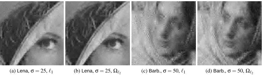
(a)Lena,σ=25,ℓ1 (b)Lena,σ=25,Ωℓ2 (c)Barb.,σ=50,ℓ1 (d)Barb.,σ=50,Ωℓ2

Figure 5: Visual comparison between the wavelet shrinkage model with theℓ1-norm and the tree-structured model, on cropped versions of the imagesLenaandBarb.. Haar wavelets are used.

This experiment does of course not provide state-of-the-art results for image denoising (see Mairal et al., 2009b, and references therein), but shows that the tree-structured regularization sig-nificantly improves the reconstruction quality for wavelets. In this experiment the convex set-ting Ωℓ2 andΩℓ∞ also outperforms the nonconvex one ℓ

tree

0 .21 We also note that the speed of our approach makes it scalable to real-time applications. Solving the proximal problem for an image with m=512_×512=262 144 pixels takes approximately 0.013 seconds on a single core of a 3.07GHz CPU ifΩis a sum ofℓ2-norms, and 0.02 seconds when it is a sum ofℓ_∞-norms. By con-trast, unstructured approaches have a speed-up factor of about 7-8 with respect to the tree-structured methods.

17. These images are used in classical image denoising benchmarks. See Mairal et al. (2009b).

18. For the convex formulations, i ranges in_{−15,−14, . . . ,15_}, while in the nonconvex case i ranges in_{−24, . . . ,48_}. 19. Denoting by MSE the mean-squared-error for images whose intensities are between 0 and 255, the PSNR is defined

as PSNR=10 log₁₀(2552_{/MSE)and is measured in dB. A gain of 1dB reduces the MSE by approximately 20%.}

20. Software available athttp://www.cns.nyu.edu/˜eero/steerpyr/.

5.4 Dictionaries of Natural Image Patches

This experiment studies whether a hierarchical structure can help dictionaries for denoising natural image patches, and in which noise regime the potential gain is significant. We aim at reconstructing corrupted patches from a test set, after having learned dictionaries on a training set of non-corrupted patches. Though not typical in machine learning, this setting is reasonable in the context of images, where lots of non-corrupted patches are easily available.22

noise 50 % 60 % 70 % 80 % 90 %

flat 19.3_±0.1 26.8_±0.1 36.7_±0.1 50.6_±0.0 72.1_±0.0 tree 18.6_±0.1 25.7_±0.1 35.0_±0.1 48.0_±0.0 65.9_±0.3

Table 2: Quantitative results of the reconstruction task on natural image patches. First row: percent-age of missing pixels. Second and third rows: mean square error multiplied by 100, respectively for classical sparse coding, and tree-structured sparse coding.

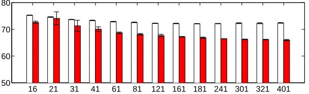
16 21 31 41 61 81 121 161 181 241 301 321 401 50

60 70 80

Figure 6: Mean square error multiplied by 100 obtained with 13 structures with error bars, sorted by number of dictionary elements from 16 to 401. Red plain bars represents the tree-structured dictionaries. White bars correspond to the flat dictionary model containing the same number of dictionary as the tree-structured one. For readability purpose, the y-axis of the graph starts at 50.

We extracted 100 000 patches of size m=8_×8 pixels from the Berkeley segmentation database of natural images (Martin et al., 2001), which contains a high variability of scenes. We then split this data set into a training set Xtr, a validation set Xval, and a test set Xte, respectively of size 50 000, 25 000, and 25 000 patches. All the patches are centered and normalized to have unitℓ2-norm.

For the first experiment, the dictionary D is learned on Xtr using the formulation of Equa-tion (10), with µ=0 for

D

µas defined in Equation (11). The validation and test sets are corrupted by removing a certain percentage of pixels, the task being to reconstruct the missing pixels from the known pixels. We thus introduce for each element x of the validation/test set, a vector ˜x, equal to x for the known pixel values and 0 otherwise. Similarly, we define ˜D as the matrix equal to D, except

for the rows corresponding to missing pixel values, which are set to 0. By decomposing ˜x on ˜D, we

obtain a sparse codeα, and the estimate of the reconstructed patch is defined as Dα. Note that this procedure assumes that we know which pixel is missing and which is not for every element x.

The parameters of the experiment are the regularization parameterλtrused during the training step, the regularization parameterλte used during the validation/test step, and the structure of the

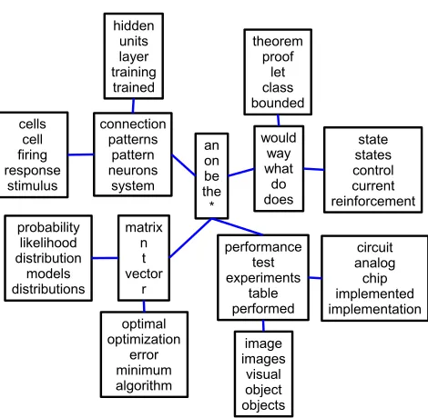
Figure 7: Learned dictionary with a tree structure of depth 5. The root of the tree is in the middle of the figure. The branching factors are p1=10, p2=2, p3=2, p4=2. The dictionary is learned on 50,000 patches of size 16×16 pixels.

tree. For every reported result, these parameters were selected by taking the ones offering the best performance on the validation set, before reporting any result from the test set. The values for the regularization parametersλtr,λte were selected on a logarithmic scale{2−10,2−9, . . . ,22}, and then further refined on a finer logarithmic scale with multiplicative increments of 2−1/4. For simplicity, we chose arbitrarily to use theℓ∞-norm in the structured normΩ, with all the weights equal to one. We tested 21 balanced tree structures of depth 3 and 4, with different branching factors p1,p2, . . . ,pd−1, where d is the depth of the tree and pk, k∈ {1, . . . ,d−1} is the number of children for the nodes at depth k. The branching factors tested for the trees of depth 3 where p1_{∈ {}5,10,20,40,60,80,100_}, p2_{∈ {}2,3_}, and for trees of depth 4, p1_{∈ {}5,10,20,40_}, p2_{∈ {}2,3_} and p3=2, giving 21 possible structures associated with dictionaries with at most 401 elements. For each tree structure, we evaluated the performance obtained with the tree-structured dictionary along with a non-structured dictionary containing the same number of elements. These experiments were carried out four times, each time with a different initialization, and with a different noise realization.