A Unified View on Multi-class Support Vector Classification
¨
Ur¨un Do˘gan [email protected]
Microsoft Research
Tobias Glasmachers [email protected]
Institut f¨ur Neuroinformatik
Ruhr-Universit¨at Bochum, Germany
Christian Igel [email protected]
Department of Computer Science University of Copenhagen, Denmark
Editor:Ingo Steinwart
Abstract
A unified view on multi-class support vector machines (SVMs) is presented, covering most prominent variants including the one-vs-all approach and the algorithms proposed by We-ston & Watkins, Crammer & Singer, Lee, Lin, & Wahba, and Liu & Yuan. The unification leads to a template for the quadratic training problems and new multi-class SVM formu-lations. Within our framework, we provide a comparative analysis of the various notions of multi-class margin and margin-based loss. In particular, we demonstrate limitations of the loss function considered, for instance, in the Crammer & Singer machine.
We analyze Fisher consistency of multi-class loss functions and universal consistency of the various machines. On the one hand, we give examples of SVMs that are, in a particular hyperparameter regime, universally consistent without being based on a Fisher consistent loss. These include the canonical extension of SVMs to multiple classes as proposed by Weston & Watkins and Vapnik as well as the one-vs-all approach. On the other hand, it is demonstrated that machines based on Fisher consistent loss functions can fail to identify proper decision boundaries in low-dimensional feature spaces.
We compared the performance of nine different multi-class SVMs in a thorough empir-ical study. Our results suggest to use the Weston & Watkins SVM, which can be trained comparatively fast and gives good accuracies on benchmark functions. If training time is a major concern, the one-vs-all approach is the method of choice.
Keywords: support vector machines, multi-class classification, consistency
1. Introduction
exist-ing approaches. It provides a thorough framework for analyzexist-ing, designexist-ing, and efficiently training multi-class SVMs.
There exist generic ways of doing multi-category classification based on arbitrary binary learning machines by combining hypotheses from independently trained binary classifiers. In contrast, the focus of this study is on multi-class extensions of SVMs that aim at gen-eralizing the notions of margin and large margin loss. These so-called all-in-one machines cast the learning problem into a single quadratic program, which allows them to take all class relationships into account simultaneously. The first of these all-in-one formulations was independently proposed by Weston and Watkins (1999), Vapnik (1998), and Breden-steiner and Bennett (1999). Crammer and Singer (2002) modified this machine, and their approach is frequently used, in particular when dealing with structured output. In addition to these popular methods, we consider the machine by Lee et al. (2004), a variant proposed by Liu and Yuan (2011), as well as multi-class maximum margin regression (Szedmak et al., 2006). The latter is equivalent to a multi-class SVM suggested by Zou et al. (2008). From a geometric point of view, the various approaches differ in the way they extend the concepts of margin and margin violation (or, to be more precise, margin-based loss) to multiple classes. Differentiating the machines form a learning-theoretical perspective is more difficult. Al-beit there have been extensions of generalization bounds derived for binary SVMs to the multi-class case (e.g., Guermeur, 2007; Do˘gan et al., 2012), these do not allow to deduce relative advantages or disadvantages of certain multi-class SVM formulations. But there are hints from theoretical analyzes of consistency. In particular, the loss function proposed by Lee et al. was the first multi-class large margin loss known to be Fisher consistent (Lee et al., 2004; Tewari and Bartlett, 2007; Liu, 2007). The only other loss functions we are aware of sharing this property are those proposed in the work of Liu and Yuan (2011). In practice, however, the decision of which multi-class SVM to use is most often not gov-erned by theoretical arguments, but by training-time considerations and the availability of efficient implementations. For instance, the canonical extension of binary SVMs to mul-tiple classes proposed by Weston and Watkins and the machine by Lee et al. are rarely used. These approaches are theoretically sound and experiments indicate that they lead to well-generalizing hypotheses, but efficient training algorithms have been lacking so far.
does not provide hints on how loss functions may affect the generalization performance of different machines. Finally, it is important to provide an extensive and unbiased empirical comparison.
This article is organized as follows. The next section presents our unifying framework, which categorizes multi-class SVMs according to their choice of multi-class loss function, margin function, and aggregation operator in subsections 2.1–2.3. Subsection 2.4 shows how the existing multi-class machines fit into our scheme. Then we derive new SVM variants suggested by the framework. Subsection 2.6 states a template for quadratic programs describing the learning problems induced by machines falling into our framework. Section 3 analyzes how different design choices affect the Fisher and universal consistency of the loss functions and the classifiers, respectively. The section closes with showcase experiments on synthetic test problems designed to highlight consequences of certain design choices. Section 4 presents an extensive experimental evaluation of various SVM variants, both with linear as well as Gaussian kernels. The theoretical as well as empirical findings finally lead us to conclusions including recommendations for the use of multi-class SVMs in practice.
2. A Framework for Multi-category SVM Classification
Multi-class SVMs construct hypothesesh:X→Y from training data (x1, y1), . . . ,(x`, y`)
∈
X×Y`
, whereX and Y are the input and label space, respectively. The data points are assumed to be sampled i.i.d. from a distributionP onX×Y. We restrict our considerations to the standard case of a finite label space and set Y = {1, . . . , d} (there exist extensions of multi-class SVMs to infinite label spaces, e.g., Bordes et al. e.g., 2008). The goal of training a multi-category SVM is to map the training data to a hypothesis minimizing the risk (generalization error) R(h) = R
X×Y
L(h(x), y) dP(x, y), where the loss function L is
typically the 0-1-loss, which is zero if both arguments are identical and one otherwise. For multi-category classification the binary SVM concept of thresholding a real-valued decision functionf :X →Rat zero is insufficient. The canonical extension tod >2 classes is to employ a vector-valued linear decision function f : X → Rd, where the maximal
component indicates the decision. Using a kernel-induced feature space, the corresponding hypothesis takes the form
h:X→Y ={1, . . . , d}; x7→arg max
c∈Y
fc(x) = arg max
c∈Y
hwc, φ(x)i+bc , (1)
where φ : X → H is a feature map into an inner product space H, w1, . . . , wd ∈ H are
class-wise weight vectors, and b1, . . . , bd∈ R are class-wise bias/offset values. The feature
map is defined by a positive definite kernel function k : X ×X → R with the property k(x, x0) =hφ(x), φ(x0)i. We presume that the arg max operator in Equation (1) returns a single class index (ties may, for example, be broken at random). To ease the notation, we define the riskR(f) to be equal to the corresponding R(h).
Adding the same function g:X→Rto all componentsfcof the decision function does
not change the decision as arg maxc∈Y n
fc(x) o
= arg maxc∈Y n
fc(x) +g(x) o
by enforcing the so-called sum-to-zero constraint
d X
c=1
fc(x) = 0 . (2)
At least for universal kernels (Steinwart, 2002a) the constraint is equivalent toPd
c=1wc= 0
and Pd
c=1bc = 0. With this constraint we have f2 = −f1 for the special case of binary classification, and the hypothesis h(x) = sign(f1(x)) maps the first class to +1 and the second to−1. Thus, the binary SVM can be recovered as a special case of the multi-class SVM, which is an important design criterion.
2.1 Multi-class Loss Functions
Support vector machines select a hypothesis by minimizing the regularized empirical risk functional
1 2kfk
2+C·
` X
i=1
L(f(xi), yi) , (3)
where L is a large-margin loss function and C > 0 is a user-defined regularization con-stant. The squared norm is defined as kfk2 = P
c∈Y kfck2 =
P
c∈Y kwck2. Most existing
approaches to multi-class large margin classification differ only in the type of loss function, which should typically be an upper bound on the 0-1-loss, lead to an optimization problem that can be solved efficiently, and vanish on an open set to allow for sparse solutions. The key observation for our unifying framework is that multi-class SVM loss functions can be decomposed into meaningful components, namely a set of margin functions for the different classes, a large-margin loss for binary problems, and an aggregation operator, combining the various target margin violations into a single loss value. This decomposition is found in all existing approaches to large margin multi-class classification. Given a labeled point (x, y)∈X×Y and the value f(x)∈Rd of the decision function, the general form of most
multi-class loss functions is
L f(x), y
= ∆Lbbin µ(f(x), y), y
,
or conceptually “L = ∆ ◦ Lbbin ◦ µ”. Here µ is a margin function, ∆ is an
aggrega-tion operator, and Lbin is a loss function for binary classification, such as the hinge loss
Lhinge(µ) = max{0,1−µ}, the squared hinge loss, or the Huber loss. With Lbbin we denote the component-wise application of this loss function to the margin values.
In the next two subsections, we formalize the concepts of margin functions and ag-gregation operators and give examples of how existing machines can be expressed in our framework.
2.2 Margin Functions
Definition 1 (margin function) A margin function is a non-constant function
µ:Rd×Y →Rd; µ= (µ1, . . . , µd)
of a prediction f(x) ∈Rd and a label y ∈Y that is linear in its first argument and fulfills
the properties:
1. ∀y∈Y : µy(f(x), y) is non-decreasing in fy(x),
2. ∀c, y ∈Y, c6=y: µc(f(x), y) is non-increasing infc(x),
3. h
∀c∈Y : µc(f(x), y)≥0 and ∃c∈Y : µc(f(x), y)>0 i
⇒
arg maxc∈Y
fc(x) =y
Due to linearity inf(x) margin functions are of the form
µc f(x), y
=
d X
m=1
νy,c,m·fm(xi)
and can thus be expressed in terms of coefficientsνy,c,m. Property 3 in the above definition
ensures that positive margins imply correct classification. Note that the reverse statement is not guaranteed, so, correct classification does not necessarily imply that all margin functions are non-negative. The definition is not as general as it may seem. If we assume an equal treatment of all classes, then the degrees of freedom in νy,c,m are drastically reduced.
The following types of margins are of primary interest:
Definition 2 (relative and absolute margins) The relative margin function is given by
µrelc (f(x), y) = 1
2 fy(x)−fc(x)
and the absolute margin function by
µabsc (f(x), y) = (
+fc(x) for c=y
−fc(x) for c∈Y \ {y} .
The corresponding coefficients are
νy,c,m=
1
2(δy,m−δc,m) (relative)
and
νy,c,m=δm,c·(2δc,y−1) =−(−1)δc,y·δm,c (absolute)
for the relative and the absolute margin, respectively, where δa,b = 1 ifa=b and δa,b = 0
otherwise denotes the Kronecker symbol. Both margin functions can be combined, as in the work of Liu and Yuan (2011). They have a number of interesting properties:
• The “own-class-margin” component µrely (f(x), y) of relative margins is always zero. For a two-class problem, the other component coincides with the margin y·f(x) of the binary SVM (with labelsy∈ {±1}and real-valued decision functionf).
• If the classification according to Equation (1) is correct, then no component of the relative margin function is negative. This implication does not necessarily hold for absolute margin functions regardless of whether the sum-to-zero constraint is enforced or not.
• It holds P
mνy,c,m = 0 for relative but not for absolute margins. Adding the same
function to all componentsfcof the decision function does not change the decision (1).
Hence it is reasonable to demand that adding the same value to all νy,c,m does not
change the margins. This property is violated for absolute margins. This renders both the sign and the absolute value of a single margin (i.e., a component of the margin function) meaningless. This issue could be addressed by enforcingP
mνy,c,m= 0 also
for absolute margins.
• In principle, the sum-to-zero constraint (2) can be avoided at the level of the decision function by shifting the coefficientsν such that they fulfill P
mνy,c,m = 0. However,
this would destroy the sparsity of the coefficients. Thus, it can be argued that the sum-to-zero constraintP
cfc= 0 is a preferable solution.
• A regularizer of the form Pd
c=1kwck2 has the effect that the optimal solution of a
relative margin SVM always fulfills the sum-to-zero constraint. This has been observed for particular machines by Guermeur (2007) and by Wu and Liu (2007), but can be shown to be true for all relative margin SVMs. Adding the same vector w to all weight vectors wc (or the same functiong(x) =hw, φ(x)i to all components fc) does
not affect relative margins and thus the empirical error term in the primal problem. Thus, to find the optimal wwe have to minimize the complexity term
d X
c=1
hwc+w, wc+wi= d X
c=1
hwc, wci+ 2· d X
c=1
hwc, wi+d· hw, wi
w.r.t. w. Setting the derivative 2·Pd
c=1wc+d·w
to zero givesw=−1dPd
c=1wc,
which results inPd
c=1(wc+w) = 0.
• Undesired situations can occur if the absolute margin function is applied without the sum-to-zero constraint. Consider, for instance, the case of all components off being negative. In this case the “own class” margin µy is negative while all “other class”
marginsµc,c6=y, are positive, and the example could still be classified correctly. This
2.3 Aggregation Operators
Definition 1 ensures that positive margins µcindicate correct classification. Therefore it is
natural to construct a large margin loss from target margin violations, defined as
vc(f(x), y) = max n
0, γy,c−µc f(x), y o
.
The target marginsγy,care typically chosen to beγy,c= 1, which we assume in the following
if not stated otherwise. The margin violations vc = Lhinge(µc(f(x), y) correspond to the
hinge loss applied to the different margin components. As indicated above, other binary SVM loss functions can be applied at this point. In this case the resulting multi-class SVMs will be compatible with the corresponding binary SVM based on that surrogate loss (e.g., the squared hinge loss is considered by Guermeur, 2012).
The dmargin violations need to be combined into a single cost value:
Definition 3 (aggregation operator) An aggregation operator is a non-constant func-tion
∆ : (R+0)d×Y →R + 0
of margin violations v= (v1, . . . , vd) and a label y∈Y with the properties
• ∆ (0, . . . ,0), y= 0, and
• ∆((v1, . . . , vd), y) is monotonically increasing in all components vi of the first argu-ment.
The following aggregation operators are employed in machines that have been proposed in the literature:
Definition 4 We define the following aggregation operators:
∆self (v1, . . . , vd), y
=vy (self operator)
∆t-max (v1, . . . , vd), y
= max
c∈Y
n vc
o
(total-max operator)
∆o-max (v1, . . . , vd), y
= max
c∈Y\{y}
n vc
o
(max-over-others operator)
∆t-sum (v1, . . . , vd), y
=X
c∈Y
vc , (total-sum operator)
∆o-sum (v1, . . . , vd), y
= X
c∈Y\{y}
vc . (sum-over-others operator)
2.4 Unification of Existing Machines
This study considers all-in-one approaches to SVM multi-class classification. These methods extend the SVM concept of large-margin classification to the multi-class case and cast the learning task as a single optimization problem. The first all-in-one methods proposed inde-pendently by Weston and Watkins (1999), Vapnik (1998, Section 10.10), and Bredensteiner and Bennett (1999) turned out to be equivalent, up to rescaling of the decision functions and the regularization parameterC >0. We refer to this method as WW or as WW-SVM. It is expressed within our framework as the machine relying on the sum operator1 applied to relative margins.
An alternative multi-class SVM was proposed by Crammer and Singer (2002). Like the WW-SVM, the CS machine takes all class relations into account simultaneously and solves a single optimization problem, however, with fewer slack variables in its primal optimization problem. It corresponds to combining relative margins with the max-over-others operator. There are two key differences between the WW- and CS-SVMs. First, the aggregation operators are different. Second, the CS-SVM has originally been defined only for hypotheses without bias term. The machine can be extended to hypotheses with bias (Hsu and Lin, 2002), but efficient training algorithms have been missing for this extension. In our frame-work we do not distinguish between hypothesis classes with and without bias; all machines are defined for both classes.
Lee, Lin and Wahba (2004) proposed a distinct approach to multi-class SVM classifica-tion. We refer to this approach as the LLW-SVM. It was the first machine to use absolute margins in an all-in-one approach. The absolute margin violations are combined under the sum-to-zero constraint by means of the sum-over-others operator.
The LLW machine was the first multi-class SVM with a classification calibrated loss function, which guarantees its Fisher consistency (Lee et al., 2004; Tewari and Bartlett, 2007; Liu, 2007; Liu and Yuan, 2011). That is, in the limit of infinite data minimal risk in the LLW sense implies minimal 0-1-risk and thus a Bayes-optimal decision rule.
The multi-class maximum margin regression (MMR) method proposed by Szedmak et al. (2006) is driven by the observation that the quadratic term
` X
i=1
` X
j=1
αiαjyiyjk(xi, xj)
in the Wolfe dual of the binary SVM (Cortes and Vapnik, 1995; Bottou and Lin, 2007) can be interpreted as the squared norm with respect to the product kernel k⊗ky, where
the “label kernel” ky : {±1} × {±1} → R is defined as ky(yi, yj) = yiyj. This is the
standard inner product on the label space Y ={−1,+1} ⊂ R. This idea is generalized to
multiple classes by considering the standard inner product onRdapplied to label prototype
vectors{yˆ1, . . . ,yˆd}=Y ⊂Rd representing the classes. This corresponds one-to-one to the
definition of a positive definite kernel ky(c, c0) = hyˆc,yˆc0i on the standardized label space Y ={1, . . . , d}. Two different sets of prototypes have been proposed, namely
ˆ yc=
r d−1
d
−1
d−1, . . . ,1, . . . , −1 d−1
and ˆyc= (0, . . . ,1, . . . ,0), where thec-th component equals 1. The first set corresponds to a
symmetric setup of unit vectors with maximal angles between prototypes, while the second setup relies on an orthonormal basis. We refer to these variants as MMR and MMR⊥, respectively. They correspond to the label kernels
ky(yi, yj) = (
1 foryi =yj
− 1
d−1 otherwise
and ky⊥(yi, yj) =δyi,yi .
Both of these machines are obtained by applying the self aggregation operator to absolute margins, where the MMR machine enforces the sum-to-zero constraint, while the MMR⊥ machine does not.
The MMR⊥ method applied to a two-class problem does typically not give the same decision function as the standard binary SVM. With its orthogonal label kernel, it explicitly ignores all interactions between classes, so that the machine effectively trainsdindependent machines, similar to one-class SVMs for the different classes.
The unique selling proposition of the MMR and MMR⊥ machines is their applicability to problems with large numbers of classes. By design, the optimization problem of the MMR machine has only`dual variables. Even better, in case of the MMR⊥ machine the problem decomposes intodindependent sub-problems. However, this means that the MMR⊥-SVM does not take any inter-class relationships in the data into account.
Our unification also captures the reinforced multicategory SVM (RM-SVM) recently proposed by Liu and Yuan (2011). This machine, or family of machines, weights two types of margin violations using a parameter γ ∈ [0,1]. In our framework, it can be viewed as relying on areinforced margin function defined as
µrc(f(x), y) = (
γfc(x) forc=y
−(1−γ)fc(x) forc∈Y \ {y}
and using the total-sum operator and the coefficients
γy,c= (
γ(d−1) forc=y
(1−γ) forc∈Y \ {y} (4)
for combining the margin violations. The sum-to-zero constraint is enforced. For γ = 0, RM equals LLW and for γ = 1 it equals MMR with a scaled target margin.
There exist several general techniques to build a multi-category classifier based on some binary classifiers, which can be chosen to be binary SVMs. The most prominent of these so-called sequential approaches are the one-versus-one (OVO) and the one-versus-all (OVA) scheme. As an OVO approach inevitably requires some additional non-canonical decision making procedure different from (1) (e.g., Hastie and Tibshirani, 1998; Platt et al., 2000; Chang and Lin, 2011) and the optimal choice of this procedure is highly task-dependent, OVO-type approaches are out of the scope of this study (error-correcting-output-codes, ECOC, provide a general framework covering OVA and many OVO methods, see Dietterich and Bakiri, 1995; Allwein et al., 2001; Passerini et al., 2004).
Usually this class is considered the “positive” class (y= +1) in the binary problem, and all other classes are mapped to the “negative” class (y=−1). The resulting decision function can be thought of as voting for the class under consideration. Let yic = +1 if c =yi and yic =−1 if c 6= yi denote the binary label of the i-th example when training the machine
separating class cfrom the rest. Then OVA constructs decision functionsfc according to
min
fc
1 2kfck
2+C·
` X
i=1
Lhinge yci ·fc(xi)
.
and plugs them into Equation (1). Solving these dindependent optimization problems at once results in a problem of type (3). This proceeding amounts to summing up the margin violations of all binary problems. Thus, OVA can be viewed as total-sum aggregation applied to absolute margins, without enforcing the sum-to-zero constraint.
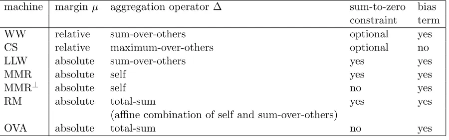
Our framework highlights the conceptual similarities and differences of the above-mentioned machines, summarized in Table 1.
machine marginµ aggregation operator ∆ sum-to-zero bias constraint term
WW relative sum-over-others optional yes
CS relative maximum-over-others optional no
LLW absolute sum-over-others yes yes
MMR absolute self yes yes
MMR⊥ absolute self no yes
RM absolute total-sum yes yes
(affine combination of self and sum-over-others)
OVA absolute total-sum no yes
Table 1: Properties of the various multi-category SVMs in terms of the unifying framework. The last column indicates the presence of the bias or offset term in the original formulation found in the literature; all machines can be formulated with or without bias term.
2.5 Completing the Picture: New Multi-class SVMs
Our unification makes it easy to construct novel loss functions based on the principles ex-tracted from existing approaches. From Table 1 it becomes obvious that some combinations of established margin functions and aggregation operators have not yet been explored. In the following, we define the corresponding machines and name them by a three-letter code, abbreviating the margin and loss types as indicated in bold in the following. The first of these new SVMs is the AMO machine, combining the absolute margin concept with the max-over-others operator. The machine can be understood as a combination of the LLW-SVM, from which it takes the margin concept, and the CS-SVM with its max-over-others aggregation.
ATS uses target margins of γy,c = 1 for y, c ∈ {1, . . . , d}, while RM-SVM uses the target
margins defined by (4) which differ depending on whether c equals y or not. The only difference between the OVA scheme and the ATS machine is the presence of the sum-to-zero constraint in the latter. Still, the ATS machine is an all-in-one machine, because its training problem is not a composition of independent (binary) problems.
2.6 Unified Dual Problem
Training SVMs amounts to solving convex quadratic optimization problems. The tradi-tional approach to solving these problems when using non-linear kernels is considering the corresponding dual formulations. In the following, we derive the Wolfe dual of the unified primal problem (3). The structure of the dual is often well-suited for the application of decomposition algorithms, which have proven to be a powerful choice for training SVMs with non-linear kernels.
For the case without sum-to-zero constraint, we arrive at the following dual problem (see supplement Section B for details):
max
α
X
i,p
γyi,p·αi,p−
1 2
X
i,p X
j,q
Myi,p,yj,q·k(xi, xj)·αi,p·αj,q (5)
s.t. ∀i, p: 0≤αi,p
∀i, r: X
p∈Pr
y
αi,p≤C
∀c:X
i,p
αi,pνyi,p,c= 0 (6)
with
Myi,p,yj,q =
X
c
νyi,p,cνyj,q,c .
The bias parametersbc can be obtained from the KKT optimality conditions.
If the sum-to-zero constraint is enforced, we obtain the same structure of the dual problem, but this time with
Myi,p,yj,q =
X
m,n
δm,n−
1 d
νyi,p,mνyj,q,n .
We call these auxiliary constants Myi,p,yj,q used in the formulation of the dual problems
kernel modifiers, because they appear as multipliers of the kernel in the dual problem. Let
the map I :{1, . . . , `} ×Py → {1, . . . , `|Py|}assign a unique index to each pair of training
pattern and constraint. We define Q∈R`|Py|×`|Py| by
QI(i,p),I(j,q) =Myi,p,yj,q·k(xi, xj) .
This matrix, together with the vector V ∈ R`|Py|, V
I(i,p) = γyi,p, defines the quadratic
objective function
W(α) =VTα−1 2α
of the dual problem, written in vector notation. The weight vectors are given by
wc= X
i,p
αi,pνyi,p,cφ(xi)−η (8)
withη=P
i,pαi,p 1dPcνyi,p,c
φ(xi) in case of a sum-to-zero constraint and zero otherwise.
For solving the problem with bias parameters, which lead to dequality constraints, we adopt the iterative problem alternation approach by Kienzle and Sch¨olkopf (2005).
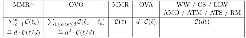
2.7 Training Complexity
Table 2 gives the asymptotic training times of various approaches. Under the assump-tion that the runtime bounds are tight, the table suggests that training MMR⊥ is faster than training OVO, which is slightly faster than MMR, which is again faster than training OVA, which is finally followed by the various all-on-one SVMs with O(d) dual variables per training example. The asymptotic nature of the runtime bounds hides factors con-siderably influencing training times in practice: Different machines often perform best for different hyper-parameters, and different concepts of separability (as discussed in Section 2 and Section 3) have an impact.
MMR⊥ OVO MMR OVA WW / CS / LLW
AMO / ATM / ATS / RM Pd
c=1C(`c)
P
1≤c<e≤dC(`c+`e) C(`) d· C(`) C(d`)
b
=d· C(`/d) =b d2· C(`/d)
Table 2: Asymptotic runtime of the training algorithms under the assumption that solving the different n-dimensional quadratic programs is in the complexity class C(n). There are good arguments to assume C(n) = O(nq) for some q between 2 and
3 (Joachims, 1998; Bottou and Lin, 2007). The number of training patterns is denoted by`, the number of examples per classcby`c, and the number of different
classes by d. In the second row the complexity is given under the assumption of (roughly) balanced classes, that is, `c∈Θ(`/d).
3. A Closer Look at Aggregation Operators and Margin Concepts
dependencyC(`) of the regularization parameterC on the data set size`, for any universal kernel, the SVM approaches the Bayes-optimal decision in the limit of infinite data. In addition to the theoretical analysis, we will empirically study the performance of the SVMs on artificial learning tasks that have been designed to highlight crucial differences between margin concepts and aggregation operators.
3.1 Fisher Consistency of Multi-class Loss Functions
In the following, we will analyze the Fisher consistency of the loss functions considered in this study. Let L(f(x), y) denote the loss function applied by a multi-class SVM for training. Letf∗:X →Rddenote a minimizer (among all measurable functions) of the risk
under the data generating distributionP. A loss function is Fisher consistent if
arg maxfc∗(x)c∈Y ⊂arg max
P(y|x)y∈Y .
In the following, we use the statements that a multi-class SVM variant and its training loss are Fisher consistent interchangeably.
The consistency of the LLW loss was established by Lee et al. (2004), and it was con-firmed by Liu (2007) that this is the only example of a Fisher consistent multi-class loss among the popular WW-, CS-, MMR-, and LLW-SVMs. The ATS machine can be viewed as belonging to the family of reinforced multicategory SVMs. Thus, the Fisher consistency of the ATS loss follows from the analysis by Liu and Yuan (2011).
We will investigate the consistency of the new machines AMO and ATM following the proceeding by Liu (2007). We adopt the short notationPy =P(y|x) for the probability of
observing class y givenx and define [t]+ = max{0, t}. It holds:
Theorem 5 Let L(f(x), y) denote either the loss function used by the AMO machine or the loss function used by the ATM machine, that is, the loss resulting from application of either the max-over-others or the total-max operator to absolute margins:
L(f(x), y) = max
c∈Y\{y}
n
vabsc (f(x), y) o
=1 + max
c∈Y\{y}
fc(x) + (AMO) or
L(f(x), y) = max
c∈Y
n
vcabs(f(x), y) o
= max (
1 + max
c∈Y\{y}{fc(x)}
+
,1−fy(x)
+ )
.
(ATM)
Then the minimizer f∗ of the corresponding risk R=E[L(f(x), y)], subject to the
sum-to-zero constraint P
c∈Y fc(x) = 0, satisfies:
• If there exists a majority class y ∈ Y such that Py >(d−1)/d, then fy∗(x) =d−1
and fc∗(x) =−1 for all c∈Y \ {y}.
• If Py <(d−1)/d for ally ∈Y, then f∗(x) = 0.
The proof, which is given in the supplementary material (Section C), works by analyzing the point-wise risk Rx=P
y∈Y P(y|x)L(f(x), y) and computing the function values fc(x)
minimizing Rx. Thus, the Fisher consistency of the loss functions used in the all-in-one
Corollary 1 It follows directly from the previous results that the AMO-loss and the ATM-loss are not Fisher consistent while the LLW-ATM-loss and the ATS-ATM-loss are Fisher consistent.
In light of the conceptual similarity between the ATS machine and the LLW-SVM, it is not surprising that the ATS-loss is Fisher consistent. However, combining margin violations by means of the maximum-operator appears to be problematic, since neither the AMO nor the ATM machine (the two “max-loss siblings” of the Fisher consistent LLW and ATS machines) share this property.
The question arises how Fisher consistency is related to (a) the margin type, (b) the aggregation of margins in the loss, and (c) the sum-to-zero constraint. Part (a) is easy to answer, since Liu (2007) has proved inconsistency of the relative margin machines (WW and CS). Thus, we focus on absolute margins in the following. We investigate the impact of the sum-to-zero constraint on the maximum and the sum of margin violations. It turns out that dropping the constraint destroys Fisher consistency:
Theorem 6 Let L(f(x), y) denote the maximum or the sum over absolute margin
viola-tions, and assume Py < 1/2 for all y ∈ Y. Then the unconstrained minimizer f∗ of the
corresponding risk R = E[L(f(x), y)] satisfies ∀c ∈ Y : fc∗(x) = −1 for the sum and
∀c∈Y :fc∗(x) = 0 for the maximum.
We do not prove this statement here; the proof is analog to the one of Theorem 5 using the techniques developed by Liu (2007). The optimal solution for the maximum operator is all zeros and satisfies the sum-to-zero constraint (cf. Theorem 5), and therefore dropping the constraint does not make any difference. However, the constraint is relevant when the sum operator is employed. The resulting solution does not sum to zero, and it is not Bayes-optimal. This result confirms the importance of the constraint for Fisher consistency. The ATS machine can be interpreted as the OVA machine with sum-to-zero constraint, and Theorem 6 covers the OVA machine, which is inconsistent in the absence of a majority class. Thus, adding the sum-to-zero constraint makes the OVA machine consistent, at the cost that the different weight vectorswc cannot be obtained independently anymore.
3.2 Universal Consistency
While Fisher consistency is just a property of the loss function, universal consistency consid-ers the whole machine including the regularizer and its impact relative to the data set size. Steinwart’s universal consistency analysis for binary SVMs builds on the fact that the hinge loss is classification calibrated for binary problems. It can be extended to multi-class SVMs with Fisher consistent losses under the assumption of the same training set size dependent choice C(`) of the regularization parameter as assumed for the binary SVMs. Thus, from Corollary 1 we get:
Theorem 7 The LLW-SVM and the ATS-SVM with universal kernel and regularization parameter chosen according to Theorem 2 by Steinwart (2002b) are universally consistent classifiers.
It can be shown that using the same rule forC(`) as in Theorem 2 from Steinwart (2002b) with a non-Fisher consistent loss does not yield a universally consistent classifier. However, this negative result does not exclude the existence of a different dependency of C on ` so that the resulting classifier is universally consistent. Thus, the question arises whether for an SVM surrogate loss function Lthere exists a dependency C(`) of the regularization parameter on the training set size such that the resulting classifier is universally consistent. In the following, we answer the question for all SVM variants covered in this study—with the surprising result that also the MMR-, WW-, and OVA-SVMs can be made consistent when operated with a completely different trade-offC(`):
Theorem 8 For the Gaussian kernel k(x, x0) = exp(−γkx−x0k2) on an input space X⊂
Rp, the machines MMR-SVM, WW-SVM, LLW-SVM, ATS-SVM, and OVA-SVM with
regularization parameterC(`)≤1/(d·`) and kernel parameterγ(`) fulfillinglim`→∞γ(`) =
∞ and lim`→∞`·γ(`)−p/2 =∞ are universally consistent classifiers.
Proof Let us first consider the all-in-one machines. The absolute values of all components of the quadratic matrixQin the dual problem (7) are upper bounded by one. All components of the dual solutionα are bounded by C(`) = 1/(d·`). The sum in the derivative
∂W(α) ∂αi,p
= 1−X
j,q
QI(i,p),I(j,q)·αj,q
runs over at most d·` summands, each of which is bounded by d1·`. Thus all gradient components are non-negative in the whole box-shaped feasible region. It follows that all dual variablesαi,p end up at the upper boundC. From Equation (8) and the definition of
the machines it can be seen that for the primal solution it holds wc= ˜wc−η˜with
• η˜=η and ˜wc=C·Pi|yi=cφ(xi) for the MMR machine,
• η˜=η−C·P
iφ(xi) and ˜wc=C·d/2· P
i|yi=cφ(xi) for the WW machine,
• η˜=η−C·P
iφ(xi) and ˜wc=C· P
i|yi=cφ(xi) for the LLW machine,
• η˜=η−C·P
iφ(xi) and ˜wc= 2C·Pi|yi=cφ(xi) for the ATS machine.
The weight vectors ˜wc are a scaled version of the kernel density estimator (KDE), which
is well known to be universally consistent. The above conditions on γ(`) translate into the preconditions of Theorem 10.1 by Devroye et al. (1996, p. 150) for the kernel width h=p1/γ(`). The KDE output fed into the arg max decision rule (1) ignores the additive constant ˜η and yields consistent classification predictions.
The OVA result can be proven in the same way. Again, all dual variables take the value C. It is easy to see that the primal SVM solution is then a scaled KDE plus a constant vector: wc = ˜wc−η˜, with ˜η = Piφ(xi) and ˜wc = 2·Pi|yi=cφ(xi). Thus, the resulting
classifier is universally consistent.
a much simpler proof than the famous universal consistency result by Steinwart (2002b). The core idea of Steinwart’s analysis is to carefully increase the modeling power of the SVM with growing number of training points so that the impact of regularizer decays to zero, while at the same time overfitting is avoided. In contrast, we keep the impact of the regu-larizer constantly high. When operating the SVM in this regime it loses its most important features, namely the large margin approach and the sparsity (Steinwart and Christmann, 2008). This may seem highly undesirable, but from the viewpoint of classification accuracy it does not matter much whether an SVM with a specific value of C works well because of a large margin or because of the consistency of KDE. Of course, KDE estimation is less sample and memory efficient than large-margin prediction. Sample efficiency is one of the primary arguments brought forward by Vapnik (1998) for preferring direct estimation of the decision boundary over a plug-in classifier based on KDE.
Theorem 8 establishes the consistency of the MMR, WW, and OVA machines, despite the Fisher inconsistency of their losses. This implies that an analysis of the loss func-tion in isolafunc-tion in terms of Fisher consistency is not sufficient for fully understanding the predictions made by these machines.
The simple trick of reverting to KDE-based prediction is not trivial, since it does not work for all large margin losses:
Theorem 9 There exists no function C(`) so that CS-SVM, AMO-SVM, or ATM-SVM become universally consistent.
Proof Consider a single-point input space X = {x0} with any kernel k(x0, x0) >0 (any positive kernel is universal on this space). Consider a problem with d = 3 classes. It is completely described by the class probabilities; w.l.o.g. they fulfill p1 ≥p2≥p3. Lemma 4 by Liu (2007) for the CS machine, and Theorem 5 for the AMO-SVM and the ATM-SVM, respectively, offer choices of these probabilities so that the minimizer of the empirical risk is f1(x0) = f2(x0) = f3(x0) = 0, with corresponding weight vectors w1 = w2 = w3 = 0. This inconsistent solution also minimizes the regularizer, and thus the regularized risk for all C >0.2
The proof lifts results on Fisher-(in)consistency from the level of the loss function to inconsistency of the actual SVM, taking the regularizer into account. The case of the MMR, WW and OVA machines treated above makes clear that this extension is non-trivial, since for these machines the regularizer makes the difference between consistency and inconsistency. We regard this type of analysis as highly relevant, since SVMs do not actually minimize the empirical risk, but instead a combination of empirical risk and a specific regularizer.
The present analysis covers the three losses involving the max-aggregation completely, since for no C (or C(`)) they result in a universally consistent SVM. On the other hand, there is a gap in our analysis of machines employing sum-aggregation losses: For`·C(`)→ ∞ Steinwart’s analysis applies, while the trivial reduction to a KDE works only for `·C(`) (asymptotically) bounded by a rather small constant, so that all target margins are always
violated. The question whether an SVM can be consistent for parameters in the gap in between these regimes is left open.
3.3 Artificial Benchmark Problems
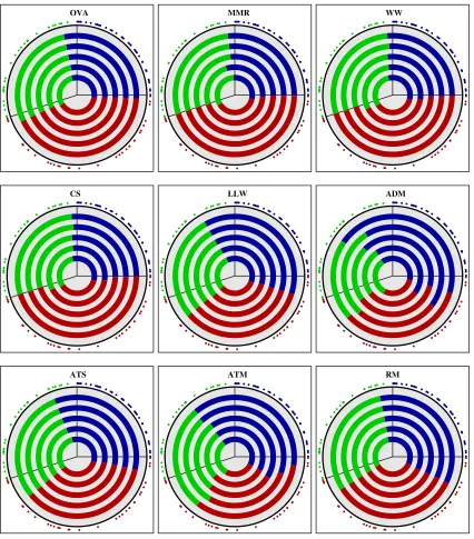
In the following, we will show experimental results on highly controlled problems with analytically defined distributions. This investigation complements and enriches the previous theoretical analysis. Some of the theoretical results on Fisher consistency of loss functions can be demonstrated in a non-asymptotic setting. The theoretical results on universal consistency require a universal kernel and thus an “arbitrarily rich” feature space. This is, however, not always the case in practice, where restricted and low-dimensional feature spaces can occur. We visualize the behavior of nine different multi-class SVMs over a range of values of the regularization parameter. The simple test problems serve as “counter examples” that help to understand when and why some of the machines deliver substantially sub-optimal solutions.
We define a basic test problem with two variants, one noise-free and one with label noise. The domain X = S1 =x ∈ R2
kxk = 1 of these test problems is the unit circle. The circle is parameterized by t∈[0,20[ through the curveβ(t) = cos(t·π/10),sin(t·π/10)
. The problem involves three classes Y = {1,2,3}, see Figure 1 and Figure 2. For the noiseless problem data points (x, y) ∈ X ×Y are generated as follows. First the label y∈Y is drawn from the uniform distribution on Y. Thenx is drawn uniformly at random from the sector Xy. The sectors have different sizes. They are defined as X1 = β([0,5)), X2 = β([5,11)), and X3 = β([11,20)). The only change for the noisy case is that 90% of the labels are reassigned uniformly at random. In other words the distribution of the x -component remains unchanged, and conditioned onx∈Xz the eventy=zhas probability
40%, while the other two cases have probabilities of 30%. In both variants of the problem it is Bayes-optimal to predict labely on sectorXy. This solution can be realized by a linear
model without offset term.
These problems are rather elementary. They are low-dimensional and thus easy to visualize. Their only difficulty lies in the uneven sector sizes. This also results in different densities of thex-components in the different sectors. This design avoids the exploitation of artificial symmetries. The construction is so that in the noisy variant there is no majority class at any point.
OVA MMR WW
CS LLW ADM
ATS ATM RM
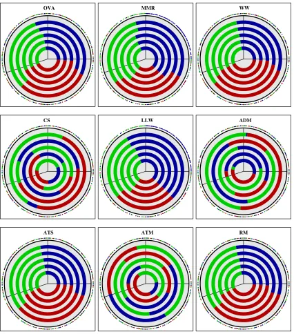
OVA MMR WW
CS LLW ADM
ATS ATM RM
Figure 1 shows that the relative margin machines WW and CS excel, in particular for high values of C. Also the MMR machine relying on the self-margin component performs well. In contrast, the absolute margin machines LLW, AMO, ATS, RM, and ATM all fail, over the whole range of parameters (despite the universal consistency of some of the approaches in rich enough feature spaces). The same defect can be observed for OVA, but in weaker form.
The reason for this failure is that the definition of absolute margins does not allow to solve the given problem without violation of the target margin. This holds even for the Bayes-optimal classifier. Thus, absolute margins are not compatible with the form of the decision function. This is obvious for the OVA approach on the circle problem, because one class cannot be separated from the others by a single linear hyperplane through the origin. It turns out that this effect is not a direct consequence of the OVA approach, but of absolute margins in general.
Figure 2 displays the performance in the presence of massive label noise. The perfor-mance of the WW machine remains good, but as expected it needs a much smaller value of C. The performance of MMR degrades a bit, while OVA does well in this case. The sub-optimal performance of the LLW machine is largely unchanged, while the closely related ATS and RM profit from the self-margin component (which by itself works well, as shown by the MMR results). Most strikingly, the CS machine with its relative margin as well as the AMO and ATM machines with their absolute margins give random predictions. All three approaches rely on maximum-based aggregation operators. This behavior is perfectly explained by the Fisher consistency results (also reflected in the proof of Theorem 5): Since there is no majority class, all losses favor the trivial solution w1 = w2 = w3 = 0. This solution is also optimal for the regularizer. Thus, it is attained for all values of C, and the figures show nothing but numerical noise. In the noisy case the combination of loss components with maximum-based aggregation operators results in guessing performance. Notably this includes the well established CS machine.
In low dimensional feature spaces we see absolute margin machines fail in the noiseless case and maximum-based aggregation operators in the noisy case.3 Despite the simplicity of the synthetic problems, only a single machine solves both cases, namely the WW approach. The simplistic OVA and MMR machines perform worse, but still satisfactory.
4. Empirical Comparison
This section empirically compares nine approaches to multi-category SVM learning, namely the sequential OVA scheme, the established all-in-one methods WW, CS, LLW, RM, and MMR, as well as the new methods called AMO, ATS, and ATM. All algorithms were implemented in theShark open source machine learning library (Igel et al., 2008). Source
code for reproducing the results can be found in the supplementary material. First, twelve standard benchmark data sets were considered for non-linear SVM learning, and careful model selection was conducted. This already makes our experiments the most extensive comparison of multi-class SVMs so far. Second, additional experiments for linear SVMs are presented later in this section.
4.1 Multi-class Benchmark Problems
The descriptive statistics of the twelve data sets used to evaluate the non-linear multi-class SVM methods are given in Section D of the supplementary material. All features of all data sets were pre-processed by rescaling to unit variance. This rescaling was done for each split into training and test data individually based on the statistics of the particular training set.
4.2 Model Selection
In all non-linear SVM experiments, Gaussian kernelskγ(x1, x2) = exp(−γ||x1−x2||2) were used. The bandwidth γ of the Gaussian kernel and the regularization parameterC of the machine were determined by nested grid search. Repeated cross-validation was employed as model selection criterion. Five-fold cross-validation was repeated ten times using ten independent random splits into five folds. This stabilizes the model selection procedure especially for small data sets. Candidate parameters were evaluated on the 5×10 validation subsets and the configuration yielding the best average performance was chosen. If any of the selected model parameters was at the grid boundary, then the grid was extended accordingly.
We set the initial grid to γ ∈ {2−12+3i|i= 0,1, . . . ,4} and C ∈ {23i|i= 0,1, . . . ,4}. Let (γ0, C0) denote the parameter configuration picked in the first stage. Then in the second stage the parameters were further refined on the gridγ ∈ {2i·γ0|i=−2,−1,0,1,2} and C ∈ {2i ·C
0|i = −2,−1,0,1,2}. For linear SVMs we applied the same approach restricted to the complexity control parameterC. The hyperparameters as determined by the grid-searches are given in Section E of the supplementary material.
Table 3 provides a comparison reflecting the computational demand of parameter tuning. It lists the total training time for computing the 5-fold cross validation error on a 5×5 grid of the outer grid search loop, centered on the optimal parameters. Training times differ by several orders of magnitude depending on the SVM variant.
Data set OVA MMR WW CS LLW AMO ATS ADS RM
Car 36.45 12.89 131.7 1027 6112 40231 2399 34046 4106
Glass 1.10 0.32 2.05 318.6 48.50 369.2 247.1 186.1 69.87
Iris 1.41 0.13 13.02 1.30 25.58 4.63 647.7 35.01 243.1 Red wine 53.87 10.51 57.68 2574 7354 75159 6486 67000 2235
Table 3: Time in seconds for computing the 5-fold cross validation error on a single core over a 5×5 grid around the optimal parameter values.
4.3 Evaluation
The multi-class SVMs were evaluated as follows. Using the best parameters found during model selection, 100 machines were trained on 100 random splits into training and test data (preserving the original set sizes).4 In this way properties of the test error distribution
can be estimated. We report empirical mean and standard deviation. Furthermore, the 100 repetitions allow to test results for significant differences. For each problem we have compared each machine to the best performing one with a paired U-test (at significance level α= 0.01). We are not interested in the test results per se; instead, the tests provide thresholds for judging performance as competitive or inferior. It must be noted that the 100 repetitions share the same data and are thus not independent. This means that the confi-dence level needs adjustment. However, the U-test still provides a meaningful thresholding mechanism.
4.4 Stopping Condition
For a fair comparison of training times of different SVMs, it is of importance to choose comparable stopping criteria for the quadratic programming. Unfortunately, this is hardly possible in the experiments presented in this study, because the quadratic programs differ. However, in the case of just two classes all machines solve the same problem. Therefore the stopping condition was selected such that for a binary problem these machines would give the same solution. The common threshold of ε= 10−3 on violations of the Karush-Kuhn-Tucker (KKT) conditions of optimality was used as stopping criterion (Bottou and Lin, 2007).
To rule out artifacts of this choice several experiments were repeated with an accuracy of ε= 10−5. These experiments did not result in improved performance. Thus, the choice of the stopping criterion may in the worst case influence training times, but not the test accuracies reported in Section 4.5 and Section 4.6.
For all non-linear machines, the maximum number of SMO iterations was limited to 10.000 times the number of dual variables. The limit for linear machines was 10 times higher.5 This was necessary to keep the grid searches computationally tractable. However, the few parameter configurations that had hit this limit corresponded to “degenerated” machines (i.e., bad solutions), typically with far too small γ and too large C. Thus, this proceeding did not influence the outcome of the model selection process.
4.5 Non-linear SVM Results
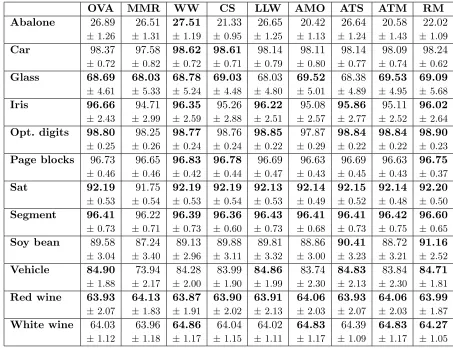
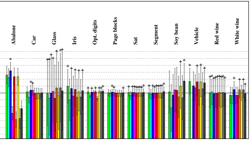
The test accuracies of all nine machines are listed in Table 4. The table also indicates whether a paired U-test judges the 100 test accuracies as significantly worse than the ma-chine with the best performance. The relative accuracies of the 9 mama-chines are represented graphically in Figure 3.
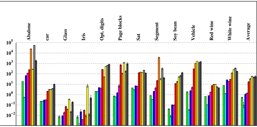
A similar plot in Figure 4 displays training times. The training times varied vastly with the choice of the hyper-parameters, that is, they were strongly dependent on the outcome of the model selection procedure. In some cases there exist configurations with similar prediction performance but different optimization times. Thus, the timing results were subject to non-negligible noise and should thus be interpreted with care.
OVA MMR WW CS LLW AMO ATS ATM RM
Abalone 26.89 26.51 27.51 21.33 26.65 20.42 26.64 20.58 22.02
±1.26 ±1.31 ±1.19 ±0.95 ±1.25 ±1.13 ±1.24 ±1.43 ±1.09 Car 98.37 97.58 98.62 98.61 98.14 98.11 98.14 98.09 98.24
±0.72 ±0.82 ±0.72 ±0.71 ±0.79 ±0.80 ±0.77 ±0.74 ±0.62
Glass 68.69 68.03 68.78 69.03 68.03 69.52 68.38 69.53 69.09
±4.61 ±5.33 ±5.24 ±4.48 ±4.80 ±5.01 ±4.89 ±4.95 ±5.68
Iris 96.66 94.71 96.35 95.26 96.22 95.08 95.86 95.11 96.02
±2.43 ±2.99 ±2.59 ±2.88 ±2.51 ±2.57 ±2.77 ±2.52 ±2.64 Opt. digits 98.80 98.25 98.77 98.76 98.85 97.87 98.84 98.84 98.90
±0.25 ±0.26 ±0.24 ±0.24 ±0.22 ±0.29 ±0.22 ±0.22 ±0.23 Page blocks 96.73 96.65 96.83 96.78 96.69 96.63 96.69 96.63 96.75
±0.46 ±0.46 ±0.42 ±0.44 ±0.47 ±0.43 ±0.45 ±0.43 ±0.37
Sat 92.19 91.75 92.19 92.19 92.13 92.14 92.15 92.14 92.20
±0.53 ±0.54 ±0.53 ±0.54 ±0.53 ±0.49 ±0.52 ±0.48 ±0.50
Segment 96.41 96.22 96.39 96.36 96.43 96.41 96.41 96.42 96.60
±0.73 ±0.71 ±0.73 ±0.60 ±0.73 ±0.68 ±0.73 ±0.75 ±0.65
Soy bean 89.58 87.24 89.13 89.88 89.81 88.86 90.41 88.72 91.16
±3.04 ±3.40 ±2.96 ±3.11 ±3.32 ±3.00 ±3.23 ±3.21 ±2.52
Vehicle 84.90 73.94 84.28 83.99 84.86 83.74 84.83 83.84 84.71
±1.88 ±2.17 ±2.00 ±1.90 ±1.99 ±2.30 ±2.13 ±2.30 ±1.81
Red wine 63.93 64.13 63.87 63.90 63.91 64.06 63.93 64.06 63.99
±2.07 ±1.83 ±1.91 ±2.02 ±2.13 ±2.03 ±2.07 ±2.03 ±1.87 White wine 64.03 63.96 64.86 64.04 64.02 64.83 64.39 64.83 64.27
±1.12 ±1.18 ±1.17 ±1.15 ±1.11 ±1.17 ±1.09 ±1.17 ±1.05
Table 4: Classification accuracies in percent of correctly classified test examples. The table lists mean values and standard deviations. In each row bold numbers indicate that the result is not significantly worse than the best one (paired U-test,α= 0.01).
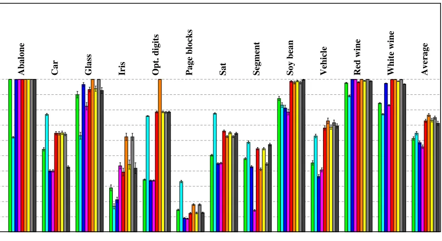
In many applications not only training times but also testing times are of relevance. The time it takes to compute the prediction of an SVM classifier is usually dominated by the kernel computations. In the multi-class case this means that sparsity in the dual variables is not enough: only variables that do not appear in any of the expansions of the weight vectorsw1, . . . , wdcan be dropped in the evaluation of the classifier. We count every
training example that is used in the construction of any of the weight vectors as a support vector. The fraction of support vectors is reported in Figure 5.
4.6 Linear SVM Results
Abalone
*
Car
*+
Glass
++++ + *+
Iris
* ++++
Opt. digits
+ + + ++*
Page blocks
*+ +
Sat
+ ++++++*
Segment
+ ++++++*
Soy bean
+ *
Vehicle
* + + +
Red wine
+*+++++++
White wine
* + + +
Figure 3: Relative accuracies of all nine machines. The average performance per data set defines the mid-line. Each dashed line marks 1% of deviation. The colored bars denote (relative) classification accuracy (higher is better). The error bars indicate the standard deviation across multiple training/test splits. The best result is indicated with a star (∗). Statistically insignificant differences to the best solution (U-test, α = 0.01) are marked with a plus sign (+). Colors represent models as follows: green (OVA), cyan (MMR), blue (WW), pink (CS), red (LLW), orange (AMO), yellow (ATS), light gray (ATM), and dark gray (RM).
Fan et al. (2008) and has been recently extended by Glasmachers and Do˘gan (2013, 2014). All linear SVM results reported in this section were obtained with an extension of the latter technique to the multi-class case.
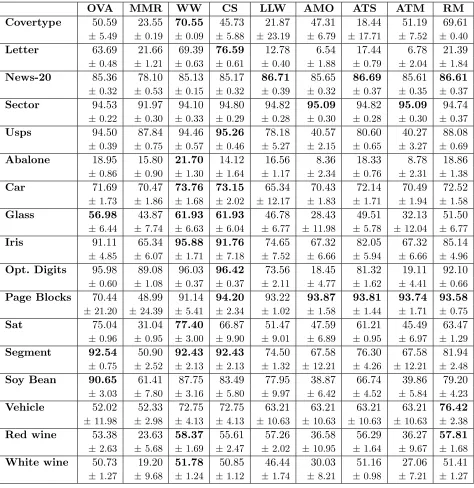
For the linear kernel case we have extended the testbed beyond the twelve problems to data sets with different characteristics, which are typically used to evaluate linear multi-class models, see supplementary material (Section E). These data sets are available from the libsvm data collection.6 We have included problems with rather low-dimenional as well as extremely high-dimensional input spaces. The test errors of the nine linear multi-class SVMs are summarized in Table 5.
10−2 10−1 100 101 102 103 104
105 Abalone car Glass Iris Opt. digits Page blocks Sat Segment Soy bean Vehicle Red wine White wine Average
Figure 4: Average training times (logarithmic scale) of all nine machines, in seconds (lower is better). Colors represent models as follows: green (OVA), cyan (MMR), blue (WW), pink (CS), red (LLW), orange (AMO), yellow (ATS), light gray (ATM), and dark gray (RM). The (geometric) average training time across all 12 problems is found on the right.
4.7 Discussion
Our results allow to compare the nine different machines from different angles. We generally view accuracy as a primary goal and training speed and prediction speed (related to sparsity of the solution) as secondary criteria.
Abalone Car Glass Iris Opt. digits Page blocks Sat Segment Soy bean Vehicle Red wine White wine Average
Figure 5: Average fraction of support vectors for all nine machines (lower is better). A bar hitting the top indicates that all points are support vectors, while a bar vanishing at the bottom indicates that no points were used as support vectors. Colors represent models as follows: green (OVA), cyan (MMR), blue (WW), pink (CS), red (LLW), orange (AMO), yellow (ATS), light gray (ATM), and dark gray (RM). The average fraction of support vectors across all 12 problems is found on the right.
calibrated LLW and RM approaches and the other absolute margin machines worked about as well as in the non-linear case. Most other problems have rather low-dimensional feature spaces. Thus, the setting comes conceptually closer to the synthetic circle problems pre-sented in Section 3. This explains the complete breakdown of some methods on some of the problems, for example, all absolute margin machines on the letter data. In accordance with the findings in Section 3, WW and CS outperformed the classification calibrated LLW, ATS and RM machines. The linear SVM results also clearly display the problems of the OVA and MMR approaches. While OVA works well at least in some cases, we have to dismiss the MMR machine completely for its consistently inferior performance. The WW and CS machines clearly performed best, again with a slight but insignificant edge for WW.
OVA MMR WW CS LLW AMO ATS ATM RM
Covertype 50.59 23.55 70.55 45.73 21.87 47.31 18.44 51.19 69.61
±5.49 ±0.19 ±0.09 ±5.88 ±23.19 ±6.79 ±17.71 ±7.52 ±0.40
Letter 63.69 21.66 69.39 76.59 12.78 6.54 17.44 6.78 21.39
±0.48 ±1.21 ±0.63 ±0.61 ±0.40 ±1.88 ±0.79 ±2.04 ±1.84
News-20 85.36 78.10 85.13 85.17 86.71 85.65 86.69 85.61 86.61
±0.32 ±0.53 ±0.15 ±0.32 ±0.39 ±0.32 ±0.37 ±0.35 ±0.37
Sector 94.53 91.97 94.10 94.80 94.82 95.09 94.82 95.09 94.74
±0.22 ±0.30 ±0.33 ±0.29 ±0.28 ±0.30 ±0.28 ±0.30 ±0.37 Usps 94.50 87.84 94.46 95.26 78.18 40.57 80.60 40.27 88.08
±0.39 ±0.75 ±0.57 ±0.46 ±5.27 ±2.15 ±0.65 ±3.27 ±0.69
Abalone 18.95 15.80 21.70 14.12 16.56 8.36 18.33 8.78 18.86
±0.86 ±0.90 ±1.30 ±1.64 ±1.17 ±2.34 ±0.76 ±2.31 ±1.38 Car 71.69 70.47 73.76 73.15 65.34 70.43 72.14 70.49 72.52
±1.73 ±1.86 ±1.68 ±2.02 ±12.17 ±1.83 ±1.71 ±1.94 ±1.58
Glass 56.98 43.87 61.93 61.93 46.78 28.43 49.51 32.13 51.50
±6.44 ±7.74 ±6.63 ±6.04 ±6.77 ±11.98 ±5.78 ±12.04 ±6.77 Iris 91.11 65.34 95.88 91.76 74.65 67.32 82.05 67.32 85.14
±4.85 ±6.07 ±1.71 ±7.18 ±7.52 ±6.66 ±5.94 ±6.66 ±4.96
Opt. Digits 95.98 89.08 96.03 96.42 73.56 18.45 81.32 19.11 92.10
±0.60 ±1.08 ±0.37 ±0.37 ±2.11 ±4.77 ±1.62 ±4.41 ±0.66
Page Blocks 70.44 48.99 91.14 94.20 93.22 93.87 93.81 93.74 93.58
±21.20 ±24.39 ±5.41 ±2.34 ±1.02 ±1.58 ±1.44 ±1.71 ±0.75 Sat 75.04 31.04 77.40 66.87 51.47 47.59 61.21 45.49 63.47
±0.96 ±0.95 ±3.00 ±9.90 ±9.01 ±6.89 ±0.95 ±6.97 ±1.29
Segment 92.54 50.90 92.43 92.43 74.50 67.58 76.30 67.58 81.94
±0.75 ±2.52 ±2.13 ±2.13 ±1.32 ±12.21 ±4.26 ±12.21 ±2.48
Soy Bean 90.65 61.41 87.75 83.49 77.95 38.87 66.74 39.86 79.20
±3.03 ±7.80 ±3.16 ±5.80 ±9.97 ±6.42 ±4.52 ±5.84 ±4.23
Vehicle 52.02 52.33 72.75 72.75 63.21 63.21 63.21 63.21 76.42
±11.98 ±2.98 ±4.13 ±4.13 ±10.63 ±10.63 ±10.63 ±10.63 ±2.38
Red wine 53.38 23.63 58.37 55.61 57.26 36.58 56.29 36.27 57.81
±2.63 ±5.68 ±1.69 ±2.47 ±2.02 ±10.95 ±1.64 ±9.67 ±1.68
White wine 50.73 19.20 51.78 50.85 46.44 30.03 51.16 27.06 51.41
±1.27 ±9.68 ±1.24 ±1.12 ±1.74 ±8.21 ±0.98 ±7.21 ±1.27
Table 5: Classification accuracies of the linear machines in percent of correctly classified test examples. The table lists mean values and standard deviations. In each row, bold numbers indicate that the result is not significantly worse than the best one (paired U-test, α= 0.01).
it was slightly faster on average in our experiments.7 Finally, the various absolute margin machines took at least an order of magnitude longer to train than WW and CS.
At least for expensive kernel functions prediction speed is governed by the sparsity of the resulting model. Figure 5 reveals that sparsity is primarily a property of the problem, while the chosen loss function has only a minor impact. Overall, multi-class models are expected to be less sparse than, for instance, binary SVMs since a training point can be dropped only if it does not appear in any of the dweight vectors. We observed significant sparsity only for the page blocks data. In comparison relative margin machines gave slightly more sparse models than absolute margin machines. The MMR self-margin machine did not stand out in this category. However, only few problems had sparse solutions at all, and inter-problem spread was much higher than differences between methods. Hence we do not see good reasons to reject any machine based on these data.
In summary, the WW and CS machines showed robust performance across all disciplines, with WW slightly ahead of CS. The MMR machine performed worst in terms of accuracy, but was fastest to train. In most cases there are no good reasons for absolute margin machines.
The results have an interesting interpretation in the unified view presented in Sec-tion 2. Differences between self, relative and absolute machine machines were much more pronounced than differences between aggregation operators. Relying only on the single self-margin component (MMR) is computationally attractive but results in rather poor prediction accuracy. Relative margins give strong machines. Consistent absolute margin machines with sum-aggregation are a viable alternative in sufficiently high-dimensional fea-ture spaces, although they are usually costly to train.
It is questionable whether a connection between asymptotic consistency and practical performance exists. This is partially observable in sum-aggregation absolute margin ma-chines performing well only in high-dimensional feature spaces. However, this condition does not seem to be necessary, since the other absolute margin machines show the same trend and also the inconsistent CS machine performs well, except for the noisy circle prob-lem (see Section 3.3). Overall, prediction performance seems to be more closely related to the applied margin concept than to uniform consistency.
Based on our empirical findings, we can recommend relative margin machines for almost all applications. We prefer the WW machine over the CS approach for its slightly more stable performance and its theoretical properties (consistency of WW with Gaussian kernel, see Theorem 8, and breakdown of CS on the noisy circle problem).
5. Conclusion
the components of the decision function sum to zero or not. All machines can be formulated with and without bias term (i.e., for linear and affine hypotheses in feature space), and we derived a unified formulation of the corresponding dual optimization problems in terms of margin concepts and aggregation operators.
Our unifying view pointed at three combinations of these features that had not been investigated. These missing machines were derived and evaluated. The new classifiers, named AMO-, ATS- and ATM-SVM, all use the absolute margin concept but consider different aggregates of the margin violations. The ATS machine, which can be viewed as one-vs-all classification with imposed sum-to-zero constraint and is closely related to RM SVMs, turns out to be Fisher consistent.
The LLW, RM, and ATS SVMs rely on a classification calibrated loss function. However, we have shown that a non-classification calibrated training loss function does not need to be a principal problem for an SVM, since the overall regularized empirical risk minimizer can still be consistent. This is the case for the maximum margin regression (MMR), one-vs-all (OVA), and Weston & Watkins (WW) machines. One may argue that for large enough amounts of data one should prefer consistent models over inconsistent large margins. It is provably impossible to “repair” the inconsistency of the Crammer & Singer (CS) multi-class SVM, AMO and ATM losses by means of SVM-style regularization.8 The MMR and WW machines, and even the OVA scheme (lacking the sum-to-zero property), turn out to be consistent classifiers when regularized properly. We argue that these results are best understood in the context of our unified view. All inconsistent machines apply the maximum operator for aggregation, while none of the consistent machines relies on this operator. Thus, our results hint at a fundamental difference between the sum and maximum aggregation operators.
Our unified learning problems lend themselves to efficient optimization algorithms. These allowed us to perform a thorough empirical comparison of the various multi-class SVMs and to draw conclusions about training times and generalization performance. We considered the LLW and RM machines in our experiments, which are typically omitted in comparison studies for training time reasons (e.g., Ding and Dubchak, 2001; Rifkin and Klautau, 2004; Statnikov et al., 2005), and we could perform proper model selection. We compared nine different multi-class SVM with Gaussian and linear kernel on a large col-lection of benchmark problems. The unified view enables a meaningful interpretation of the results by relating them to margin concepts and aggregation operators. We find that relative margin machines are superior for the linear kernel, and that sum-based aggrega-tion generally outperforms the maximum approach. Our empirical and theoretical results support the following recommendations:
The standard all-in-one multi-class WW SVM should be used as the default since it gives robust performance at moderate training times. It can be trained at least as fast as the popular CS SVM while giving at least as good generalization results and having nicer theoretical properties (which can matter in practice as shown on artificial test problems and when using a linear kernel). The simplistic OVA method can be a viable alternative; it delivers slightly worse results on average while being a little faster to train. If training time is a major concern then the MMR machine may seem like the best option. However,
its performance can be so poor that even sub-sampling the data in combination with WW or OVA may be a better approach.
With universal kernels and in general in extremely high-dimensional feature spaces the LLW and RM machines with their classification calibrated losses are usually on par with WW and CS and thus promising candidates. However, training may be infeasible for large data sets, for its more than ten times longer training times compared to WW and CS.
Acknowledgments
Tobias Glasmachers acknowledges support by the Mercator Research Center Ruhr (MER-CUR), project Pr-2013-0015, and Christian Igel from The Danish Council for Independent Research (DFF) through the project Surveying the sky using machine learning (SkyML).
References
E. L. Allwein, R. E. Schapire, and Y. Singer. Reducing multiclass to binary: A unifying approach for margin classifiers. Journal of Machine Learning Research, 1:113–141, 2001.
A. Bordes, N. Usunier, and L. Bottou. Sequence labelling SVMs trained in one pass. In W. Daelemans, B. Goethals, and K. Morik, editors, Machine Learning and Knowledge
Discovery in Databases, volume 5211 ofLNCS, pages 146–161. Springer, 2008.
B. E. Boser, I. M. Guyon, and V. N. Vapnik. A training algorithm for optimal margin classifiers. In Proceedings of the Fifth Annual Workshop on Computational Learning
Theory (COLT 1992), pages 144–152. ACM, 1992.
L. Bottou and C. J. Lin. Support vector machine solvers. In L. Bottou, O. Chapelle, D. DeCoste, and J. Weston, editors, Large Scale Kernel Machines, pages 1–28. MIT Press, 2007.
E. J. Bredensteiner and K. P. Bennett. Multicategory classification by support vector machines. Computational Optimization and Applications, 12(1):53–79, 1999.
C.-C. Chang and C.-J. Lin. LIBSVM: a library for support vector machines. ACM
Trans-actions on Intelligent Systems and Technology, 2(3):27, 2011.
C. Cortes and V. Vapnik. Support-vector networks.Machine Learning, 20(3):273–297, 1995.
K. Crammer and Y. Singer. On the algorithmic implementation of multiclass kernel-based vector machines. Journal of Machine Learning Research, 2:265–292, 2002.
L. Devroye, L. Gyorfi, and G. Lugosi. A probabilistic theory of pattern recognition. Springer Verlag, 1996.
T. G. Dietterich and G. Bakiri. Solving multiclass learning problems via error-correcting output codes. Journal of Artificial Intelligence Research, 2(263):286, 1995.
¨
U. Do˘gan, T. Glasmachers, and C. Igel. A note on extending generalization bounds for binary large-margin classifiers to multiple classes. In P. A. Flach, T. De Bie, and N. Cris-tianini, editors, European Conference on Machine Learning and Principles and Practice
of Knowledge Discovery in Databases (ECML-PKDD 2012), volume 7523 ofLNCS, pages
122–129. Springer, 2012.
R. E. Fan, K.W. Chang, C. J. Hsieh, X.R. Wang, and C. J. Lin. LIBLINEAR: A library for large linear classification. Journal of Machine Learning Research, 9:1871–1874, 2008.
T. Glasmachers and ¨U. Do˘gan. Accelerated coordinate descent with adaptive coordinate frequencies. InProceedings of the Fifth Asian Conference on Machine Learning (ACML), JMLR W&CP, 2013.
T. Glasmachers and ¨U. Do˘gan. Coordinate Descent with Online Adaptation of Coordinate Frequencies. Technical Report arXiv:1401.3737, arxiv.org, 2014.
Y. Guermeur. VC theory for large margin multi-category classifiers. Journal of Machine
Learning Research, 8:2551–2594, 2007.
Y. Guermeur. A generic model of multi-class support vector machine.International Journal
of Intelligent Information and Database Systems (IJIIDS), 6:555–577, 2012.
T. Hastie and R. Tibshirani. Classification by pairwise coupling. Annals of Statistics, 26 (2):451–471, 1998.
S. I. Hill and A. Doucet. A framework for kernel-based multi-category classification.Journal
of Artificial Intelligence Research, 30(1):525–564, 2007.
C. J. Hsieh, K.W. Chang, C. J. Lin, S.S. Keerthi, and S. Sundararajan. A dual coordinate descent method for large-scale linear SVM. In Proceedings of the 25th International
Conference on Machine learning (ICML), pages 408–415. ACM, 2008.
C. W. Hsu and C. J. Lin. A comparison of methods for multiclass support vector machines.
IEEE Transactions on Neural Networks, 13(2):415–425, 2002.
C. Igel, T. Glasmachers, and V. Heidrich-Meisner. Shark. Journal of Machine Learning
Research, 9:993–996, 2008.
T. Joachims. Making large-scale SVM learning practical. In B. Sch¨olkopf, C. Burges, and A. Smola, editors, Advances in Kernel Methods – Support Vector Learning, chapter 11, pages 169–184. MIT Press, 1998.
W. Kienzle and B. Sch¨olkopf. Training support vector machines with multiple equality constraints. In Machine Learning: ECML 2005, volume 3720 of LNCS, pages 182–193. Springer, 2005.
Y. Lee, Y. Lin, and G. Wahba. Multicategory support vector machines: Theory and appli-cation to the classifiappli-cation of microarray data and satellite radiance data. Journal of the