Sparse Single-Index Model

Sparse Single-Index Model

Pierre Alquier [email protected]

School of Mathematical Sciences University College Dublin James Joyce Library, Belfield Dublin 4, Ireland

G´erard Biau∗ [email protected]

LSTA, LPMA and Institut universitaire de France Universit´e Pierre et Marie Curie – Paris VI Boˆıte 158, Tour 15-25, 2`eme ´etage

4 place Jussieu, 75252 Paris Cedex 05, France

Editor:John Shawe-Taylor

Abstract

Let(X,Y)be a random pair taking values inRp×R. In the so-called single-index model, one has Y=f⋆(θ⋆T_{X) +W, where f}⋆_{is an unknown univariate measurable function,θ}⋆_{is an unknown} vec-tor inRd, andW denotes a random noise satisfyingE[W|X] =0. The single-index model is known to offer a flexible way to model a variety of high-dimensional real-world phenomena. However, de-spite its relative simplicity, this dimension reduction scheme is faced with severe complications as soon as the underlying dimension becomes larger than the number of observations (“plarger than n” paradigm). To circumvent this difficulty, we consider the single-index model estimation prob-lem from a sparsity perspective using a PAC-Bayesian approach. On the theoretical side, we offer a sharp oracle inequality, which is more powerful than the best known oracle inequalities for other common procedures of single-index recovery. The proposed method is implemented by means of the reversible jump Markov chain Monte Carlo technique and its performance is compared with that of standard procedures.

Keywords: single-index model, sparsity, regression estimation, PAC-Bayesian, oracle inequality, reversible jump Markov chain Monte Carlo method

1. Introduction

Let

D

n={(X1,Y1), . . . ,(Xn,Yn)}be a collection of independent observations, distributed as a generic independent pair(X,Y)taking values inRp_{×Rand satisfyingEY}2_{<∞. Throughout, we letPbe} the distribution of (X,Y), so that the sample

D

n is distributed according to P⊗n. In the regres-sion function estimation problem, the goal is to use the data

D

n in order to construct an estimate

rn:Rp→Rof the regression functionr(x) =E[Y|X=x]. In the classical parametric linear model, one assumes

Y =θ⋆T_X+W,

whereθ⋆_{= (θ}⋆

1, . . . ,θ⋆p)T ∈RpandE[W|X] =0. Here

r(x) =θ⋆T_x=

p

∑

j=1 θ⋆_jxj

is a linear function of the components ofx= (x1, . . . ,xp)T. More generally, we may define

Y = f⋆(θ⋆TX) +W, (1)

where f⋆is an unknown univariate measurable function. This is the celebrated single-index model, which is recognized as a particularly useful variation of the linear formulation and can easily be interpreted: The model changes only in the directionθ⋆, and the way it changes in this direction is described by the function f⋆. This model has applications to a variety of fields, such as discrete choice analysis in econometrics and dose-response models in biometrics, where high-dimensional regression models are often employed. There are too many references to be included here, but the monographs of McCullagh and Nelder (1983) and Horowitz (1998) together with the references H¨ardle et al. (1993), Ichimura (1993), Delecroix et al. (2006), Dalalyan et al. (2008) and Lopez (2009) will provide the reader with good introductions to the general subject area.

One of the main advantages of the single-index model is its supposed ability to deal with the problem of high dimension (Bellman, 1961). It is known that estimating the regression function is especially difficult whenever the dimensionpofXbecomes large. As a matter of fact, the optimal mean square convergence raten−2k/(2k+p) for the estimation of ak-times differentiable regression function converges to zero dramatically slowly if the dimension p is large compared to k. This leads to an unsatisfactory accuracy of estimation for moderate sample sizes, and one possibility to circumvent this problem is to impose additional assumptions on the regression function. Thus, in particular, ifr(x) = f⋆(θ⋆T_{x)holds for everyx∈R}p_{, then the underlying structural dimension of the} model is 1 (instead of p) and the estimation ofr can hopefully be performed easier. In this regard, it is shown in Ga¨ıffas and Lecu´e (2007) that the optimal rate of convergence over the single-index model class isn−2k/(2k+1)(instead ofn−2k/(2k+p)), thereby answering a conjecture of Stone (1982). Nevertheless, practical estimation of the link function f⋆ and the index θ⋆ still requires a de-gree of statistical smoothing. Perhaps the most common approach to reach this goal is to use a nonparametric smoother (for instance, a kernel or a local polynomial method) to construct an ap-proximation ˆfnof f⋆, then substitute ˆfninto an empirical version Rn(θ) of the mean square error

R(θ) =E[Y₋f(θT_X)]2_{, and finally choose ˆθ}

n to minimize Rn(θ) (see, e.g., H¨ardle et al., 1993; Delecroix et al., 2006, where the procedure is discussed in detail). The rationale behind this type of two-stage approach, which is asymptotic in spirit, is that it produces a√n-consistent estimate ofθ, thereby devolving the difficulty to the simpler problem of computing a good estimate for the one-dimensional function f⋆. However, the relative simplicity of this strategy is accompanied by severe difficulties (overfitting) when the dimension pbecomes larger than the number of observations n. Estimation in this setting (called “plarger thann” paradigm) is generally acknowledged as an im-portant challenge in contemporary statistics, see, for example, the recent monograph of B¨uhlmann and van de Geer (2011). In fact, this drawback considerably reduces the ability of the single-index model to behave as an effective dimension reduction technique.

the original image. Such signals have few nonzero coefficients and can therefore be described as sparse in the signal domain (see, for instance, Bruckstein et al., 2009). Similarly, recent advances in high-throughput technologies—such as array comparative genomic hybridization—indicate that, despite the huge dimensionality of problems, only a small number of genes may play a role in deter-mining the outcome and be required to create good predictors (van’t Veer et al., 2002, for instance). Sparse estimation is playing an increasingly important role in the statistics and machine learning communities, and several methods have recently been developed in both fields, which rely upon the notion of sparsity (e.g., penalty methods like the Lasso and Dantzig selector, see Tibshirani, 1996; Cand`es and Tao, 2005; Bunea et al., 2007; Bickel et al., 2009, and the references therein).

In the present document, we consider the single-index model (1) from a sparsity perspective, that is, we assume thatθ⋆_{has only a few coordinates different from 0. In the dimension reduction} scenario we have in mind, the ambient dimensionpcan be very large, much larger than the sample sizen, but we believe that the representation is sparse, that is, that very few coordinates ofθ⋆ _are nonzero. This assumption is helpful at least for two reasons: Ifpis large and the number of nonzero coordinates is small enough, then the model is easier to interpret and its efficient estimation becomes possible. Our setting is close in spirit of the approach of Cohen et al. (2012), who study approxi-mation from queries of functions of the form f(θT_{x), whereθis approximately sparse (in the sense} that it belongs to a weak-ℓpspace). However, these authors do not provide any statistical study of their model. Our modus operandi will rather rely on the so-called PAC-Bayesian approach, origi-nally developed in the classification context by Shawe-Taylor and Williamson (1997), McAllester (1998) and Catoni (2004, 2007). This strategy was further investigated for regression by Audibert (2004) and Alquier (2008) and, more recently, worked out in the sparsity framework by Dalalyan and Tsybakov (2008, 2012) and Alquier and Lounici (2011). The main message of Dalalyan and Tsybakov (2008, 2012) and Alquier and Lounici (2011) is that aggregation with a properly chosen prior is able to deal nicely with the sparsity issue. Contrary to procedures such as the Lasso, the Dantzig selector and other penalized least square methods, which achieve fast rates under rather restrictive assumptions on the Gram matrix associated to the predictors, PAC-Bayesian aggregation requires only minimal assumptions on the model. Besides, it is computationally feasible even for a large pand exhibits good statistical performance.

The paper is organized as follows. In Section 2, we first set out some notation and introduce the single-index estimation procedure. Then we state our main result (Theorem 2), which offers a sparsity oracle inequality more powerful than the best known oracle inequalities for other common procedures of single-index recovery. Section 3 is devoted to the practical implementation of the estimate via a reversible jump Markov chain Monte Carlo (MCMC) algorithm, and to numerical experiments on both simulated and real-life data sets. In order to preserve clarity, proofs have been postponed to Section 4 and the description of the MCMC method in its full length is given in the Appendix Section 5.

Note finally that our techniques extend to the case of multiple-index models, of the form

Y = f⋆(θ⋆₁TX, . . . ,θ⋆_mTX) +W,

2. Sparse Single-index Estimation

We start this section with some notation and basic requirements.

2.1 Notation

Throughout the document, we suppose that the recorded data

D

n is generated according to the single-index model (1). More precisely, for eachi=1, . . . ,n,

Yi= f⋆(θ⋆TXi) +Wi,

where f⋆ is a univariate measurable function, θ⋆ _{is a p-variate vector, andW}

1, . . . ,Wn are inde-pendent copies ofW. We emphasize that it is implicitly assumed that the observations are drawn according to the true model under study.

Recall that, in model (1),E[W_|X] =0 and, consequently, thatEW=0. However, the distribution ofW(in particular, the variance) may depend onX. We shall not precisely specify this dependence, and will rather require the following condition on the distribution ofW.

Assumption N.There exist two positive constantsσandLsuch that, for all integersk_≥2,

Eh|W_|k_|Xi_≤k! 2σ

2_Lk−2_.

Observe that AssumptionNholds in particular ifW=Φ(X)ε, whereεis a standard Gaussian random variable independent ofXandΦ(X)is almost surely bounded.

Let_kθ_k1denote theℓ1-norm of the vectorθ= (θ1, . . . ,θp)T, that is,kθk1=∑p_j=1|θj|. Without loss of generality, it will be assumed throughout the document that the indexθ⋆ belongs to

S

_1,+p , where

S

_1,+p is the set of all θ_∈Rp such that _kθ_k1 =1 and the first nonzero coordinate of θ is positive.

Denoting by _kX_k∞ the supremum norm of X, we will also require that the random variable

kX_k∞is almost surely bounded by a constant which, without loss of generality, can be taken equal to 1. Moreover, it will also be assumed that the link function f⋆is bounded by some known positive constantC. Thus, letting_kf⋆_k∞be the functional supremum norm of f⋆over[−1,1], we set: Assumption B.The condition_kX_k∞≤1 holds almost surely and there exists a positive constantC larger than 1 such that_kf⋆_k∞≤C.

Remark 1 To keep a sufficient degree of clarity, no attempt was made to optimize the constants.

In particular, the requirement C_≥1 is purely technical. It is always satisfied by taking C =

max(_kf⋆_k∞,1).

In order to approximate the link function f⋆, we shall use the vector space

F

spanned by a given countable dictionary of measurable functions_{ϕj}∞j=1. Put differently, the approximation space

F

is the set of (finite) linear combinations of functions of the dictionary. Eachϕj of the collection is assumed to be defined on[₋1,1]and to take values in[₋1,1]. To avoid getting into too much tech-nicalities, we will also assume that eachϕjis differentiable and such that, for some positive constant

ℓ,_kϕ′

jk∞≤ℓ×j. This assumption is satisfied by the (non-normalized) trigonometric system

Finally, for any measurable f:_Rp_→Randθ∈

_S

p

1,+, we let

R(θ,f) =E

h

Y₋f(θT_X)2i

and denote by

Rn(θ,f) =

1

n

n

∑

i=1

Yi−f(θTXi)

2

the empirical counterpart ofR(θ,f)based on the sample

D

n.

2.2 Estimation Procedure

We are now in a position to describe our estimation procedure. The method which is presented here is inspired by the approach developed by Catoni (2004, 2007). It strongly relies on the choice of a probability measureπon

S

_1,+p ×

F

, called the prior, which in our framework should enforce the sparsity properties of the target regression function. With this objective in mind, we first let

dπ(θ,f) =dµ(θ)dν(f),

that is, we assume that the distribution over the indexes is independent of the distribution over the link functions. With respect to the parameterθ, we put

dµ(θ) =

p

∑

i=1

10−i

∑

I_⊂{1,...,p_},|I_|=i

p i

−1

dµI(θ)

1₋(₁₀1)p , (2)

where_|I_|denotes the cardinality ofI and dµI(θ)is the uniform probability measure on the set

S

_1,+p (I) =_{θ= (θ1, . . . ,θp)∈

S

1,+p :θj=0 if and only if j∈/I}.

We see that

S

_1,+p (I) may be interpreted as the set of “active” coordinates in the single-index re-gression ofY onX, and note that the prior on

S

_1,+p is a convex combination of uniform probability measures on the subsets

S

_1,+p (I). The weights of this combination depend only on the size of the active coordinate subsetI. As such, the value_|I_|characterizes the sparsity of the model: The smaller

|I_|, the smaller the number of variables involved in the model. The factor 10−i penalizes models of high dimension, in accordance with the sparsity idea.

The choice of the prior νon

F

is more involved. To begin with, we define, for any positive integerM_≤nand allΛ>0,

B

M(Λ) =

(

(β1, . . . ,βM)∈RM: M

∑

j=1

j|βj| ≤ΛandβM6=0

)

.

Next, we let

F

M(Λ)⊂

F

be the image of

B

M(Λ)by the map

ΦM :RM →

F

It is worth pointing out that, roughly, Sobolev spaces are well approximated by

F

M(Λ)asMgrows (more on this in Section 2.3). Finally, we defineνM(df)on the set

F

M(C+1)as the image of the uniform measure on

B

M(C+1)induced by the mapΦM, and take

dν(f) =

n

∑

M=1

10−MdνM(f)

1₋(₁₀1)n . (3)

Some comments are in order here. First, we note that the priorπ is defined on

S

_1,+p _×

F

n(C+1) endowed with its canonical Borelσ-field. The choice ofC+1 instead ofCin the definition of the prior support is essentially technical. This bound ensures that when the target f⋆belongs to

F

n(C), then a small ball around it is contained in

F

n(C+1). It could be safely replaced byC+un, where

{un}∞_n=1is any positive sequence vanishing sufficiently slowly asn→∞. Next, the integerMshould be interpreted as a measure of the “dimension” of the function f—the largerM, the more complex the function—and the prior ν adapts again to the sparsity idea by penalizing large-dimensional functions f. The coefficients 10−i and 10−M which appear in (2) and (3) show that more complex models have a geometrically decreasing influence. Note however that the value 10, which has been chosen because of its good practical results, is somehow arbitrary. It could be, in all generality, replaced by a more general coefficient α at the price of a more technical analysis (and with no consequences on the rates of convergence). Finally, we observe that, for each f =∑Mj=1βjϕj ∈

F

M(C+1),

kf_k∞≤ M

∑

j=1

|βj| ≤C+1.

Now, let λbe a positive real number, called the inverse temperature parameter hereafter. The estimates ˆθ_λand ˆf_λofθ⋆_{and f}⋆_{, respectively, are simply obtained by randomly drawing}

(θˆλ,fˆλ)∼ρˆλ,

where ˆρ_λis the so-called Gibbs posterior distribution over

S

_1,+p ×

F

n(C+1), defined by the proba-bility density

d ˆρλ

dπ(θ,f) =

exp[₋λRn(θ,f)]

Z

exp[₋λRn(θ,f)]dπ(θ,f)

.

[The notation d ˆρ_λ/dπmeans the density of ˆρ_λwith respect toπ.] The estimate(_θˆ_λ,fˆ_{λ)has a simple} interpretation. Firstly, the level of significance of each pair(θ,f)is assessed via its least square error performance on the data

D

n. Secondly, a Gibbs distribution with respect to the priorπenforcing those pairs(θ,f) with the most empirical significance is assigned on the space

S

_1,+p ×

F

n(C+1). Finally, the resulting estimate is just a random realization (conditional to the data) of this Gibbs posterior distribution.

2.3 Sparsity Oracle Inequality

For anyI_{⊂ {}1, . . . ,p_}and any positive integerM_≤n, we set

θ⋆_I,M,f_I⋆_,M∈arg min (θ,f)∈S₁p_,+(I)×FM(C)

At this stage, it is very important to note that, for eachM, the infimum f_I⋆_,M is defined on

F

M(C), whereas the prior charges a slightly bigger set, namely

F

M(C+1).

The main result of the paper is the following theorem. Here and everywhere, the wording “with probability 1₋δ” means the probability evaluated with respect to the distributionP⊗n_{of the} data

D

n andthe conditional probability measure ˆρλ. Recall thatℓis a positive constant such that

kϕ′_jk∞≤ℓ×j.

Theorem 2 Assume that AssumptionNand AssumptionBhold. Set

w=8(2C+1)max[L,2C+1]

and take

λ= n

w+2[(2C+1)2_+4σ2_]. (4)

Then, for allδ_∈]0,1[, with probability at least1₋δwe have

R(θˆλ,fˆλ)−R(θ⋆,f⋆)≤Ξ inf

I⊂ {1, . . . ,p}

1≤M≤n

(

R(θ⋆_I,M,f_I⋆_,M)₋R(θ⋆,f⋆)

+Mlog(Cn) +|I|log(pn) +log 2 δ

n

)

,

whereΞis a positive constant, depending on L, C,σandℓonly.

Remark 3 Interestingly enough, analysis of the estimate(θˆλ,fˆλ)is still possible when Assumption

Nis not satisfied. Indeed, even if Bernstein’s inequality (see Lemma 5) is not valid, a recent

pa-per by Seldin et al. (2011) provides us with a nice alternative inequality assuming less restrictive assumptions. However, we would then suffer a loss in the upper bound of Theorem 2. It is also in-teresting to note that recent results by Audibert and Catoni (2011) allow the study of PAC-Bayesian

estimates without AssumptionN. However, the results of these authors are valid for linear models

only, and it is therefore not clear to what extent their technique can be transposed to our setting.

Theorem 2 can be given a simple interpretation. Indeed, we see that if there is a “small”Iand a “small”Msuch that R(θ⋆

I,M,fI⋆,M) is close toR(θ⋆,f⋆), thenR(θˆλ,fˆλ) is also close toR(θ⋆,f⋆) up to terms of order 1/n. However, if no suchI orMexists, then one of the termsMlog(Cn)/n

and_|I_|log(pn)/nstarts to dominate, thereby deteriorating the general quality of the bound. A good approximation with a “small”I is typically possible whenθ⋆_{is sparse or, at least, when it can be} approximated by a sparse parameter. On the other hand, a good approximation with a “small”Mis possible if f⋆has a sufficient degree of regularity.

To illustrate the latter remark, assume for instance that_{ϕj}∞j=1is the (non-normalized) trigono-metric system and suppose that the target f⋆belongs to the Sobolev ellipsoid, defined by

W

k,6C

2 π2

=

(

f_∈L2([−1,1]): f=

∞

∑

j=1

βjϕj and ∞

∑

j=1

j2kβ2_{j ≤}6C

2 π2

)

for some unknown regularity parameter k_≥2 (see, e.g., Tsybakov, 2009). Observe that, in this context, the approximation sets

F

M(C+1)take the form

F

M(C+1) =

(

f_∈L2([−1,1]): f=

M

∑

j=1 βjϕj,

M

∑

j=1

j_|βj| ≤C+1 andβM6=0

)

It is important to note that the regularity parameterkis assumed to be unknown, and this casts our results in the so-called adaptive setting. The following additional assumption will be needed:

Assumption D. The random variable θ⋆T_{X has a probability density on [−1,1], bounded from} above by a positive constantB.

Last, we letI⋆be the setI such thatθ⋆_∈

_S

p

1,+(I)and setkθ⋆k0=|I⋆|.

Corollary 4 Assume that AssumptionN, AssumptionBand AssumptionDhold. Suppose also that

f⋆ belongs to the Sobolev ellipsoid

W

(k,6C2/π2_{), where the real number k≥2is an (unknown)}

regularity parameter. Set w=8(2C+1)max[L,2C+1]and takeλas in (4). Then, for allδ_∈]0,1[,

with probability at least1₋δwe have

R(θˆ_λ,fˆλ)−R(θ⋆,f⋆)≤Ξ′

(

log(Cn)

n

_2k2₊k₁

+kθ ⋆_k

0log(pn)

n +

log 2_δ

n

)

, (5)

whereΞ′is a positive constant, depending on L, C,σ,ℓand B only.

As far as we are aware, all existing methods achieving rates of convergence similar to the ones provided by Corollary 4 are valid in an asymptotic setting only (pfixed andn_→∞). The strength of Corollary 4 is to provide a finite sample bound and to show that our estimate still behaves well in a nonasymptotic situation if the intrinsic dimension (i.e., the sparsity) is small with respect ton. To understand this remark, just assume that pis a function ofnsuch that p_→∞asn_→∞. Whereas a classical asymptotic approach cannot say anything useful about this situation, our bounds still provide some information, provided the model is sparse enough (i.e., _kθ⋆_k

0 is sufficiently small with respect ton).

We see that, asymptotically (p fixed andn_→∞), the leading term on the right-hand side of inequality (5) is(log(n)/n)2k2+k1_{. This is the minimax rate of convergence over a Sobolev class, up}

to a log(n)factor. However, whennis “small” andθ⋆is not sparse (i.e.,_kθ⋆_k0is not “small”), the term_kθ⋆_k

0log(pn)/nstarts to emerge and cannot be neglected. Put differently, in large dimension, the estimation ofθ⋆ _{itself is a problem—this phenomenon is not taken into account by asymptotic} studies.

It is worth mentioning that the approach developed in the present article does not offer any guar-antee on the point of view of variable (feature) selection. To reach this objective, an interesting route to follow is the sufficient dimension reduction (SDR) method proposed by Chen et al. (2010), which can be applied to the single-index model to estimate consistently the parameterθ⋆_{and perform} vari-able selection in a sparsity framework. Note however that such results require strong assumptions on the distribution of the data.

Finally, it should be stressed that the choice ofλin Theorem 2 and Corollary 4 is not the best possible and may eventually be improved, at the price of a more technical analysis however.

3. Implementation and Numerical Results

3.1 Implementation via Reversible Jump MCMC

The use of MCMC methods has become a popular way to compute Bayesian estimates. For an introduction to the domain, one should refer to the comprehensive monograph of Marin and Robert (2007) and the references therein. Importantly, in this computational framework, an adaptation of the well-known Hastings-Metropolis algorithm to the case where the posterior distribution gives mass to several models of different dimensions was proposed by Green (1995) under the name Re-versible Jump MCMC (RJMCMC) method. In the PAC-Bayesian setting, MCMC procedures were first considered by Catoni (2004), whereas Dalalyan and Tsybakov (2008, 2012) and Alquier and Lounici (2011) explore their practical implementation in the sparse context using Langevin Monte Carlo and RJMCMC, respectively. Regarding the single-index model, MCMC algorithms were used to compute Bayesian estimates by Antoniadis et al. (2004) and, more recently, by Wang (2009), who develop a fully Bayesian method to analyze the single-index model. Our implementation technique is close in spirit to the one of Wang (2009).

As a starting point for the approximate computation of our estimate, we used the RJMCMC method of Green (1995), which is in fact an adaptation of the Hastings-Metropolis algorithm to the case where the objective posterior probability distribution (here, ˆρλ) assigns mass to several different models. The idea is to start from an initial given pair(θ(0)_,f(0)_)∈

_S

p

1,+×

F

n(C+1)and then, at each step, to iteratively compute(θ(t+1)_,f(t+1)_)from(θ(t)_,f(t)_{)via the following chain of} rules:

• Sample a random pair (τ(t)_,h(t)_{) according to some proposal conditional density}

kt(.|(θ(t),f(t)))with respect to the priorπ;

• Take

(θ(t+1)_,f(t+1)_{) =}

(τ(t)_,h(t)_{) with probabilityα}

t

(θ(t)_,f(t)_{) with probability 1−α}

t,

where

αt=min 1,

dρˆλ

dπ(τ(t),h(t))×kt (θ(t),f(t))|(τ(t),h(t))

dρˆλ

dπ(θ(t),f(t))×kt (τ(t),h(t))|(θ(t),f(t))

!

.

This protocol ensures that the sequence_{(θ(t)_,f(t)_)}∞

t=0is a Markov chain with invariant probability distribution ˆρλ (see, e.g., Marin and Robert, 2007). A usual choice is to take kt ≡k, so that the Markov chain is homogeneous. However, in our context, it is more convenient to let kt =k1 ift is odd and kt =k2 iftis even. Roughly, the effect of k1 is to modify the indexθ(t) whilek2 will essentially act on the link function f(t). While the ideas underlying the proposal densitiesk1andk2 are quite simple, a precise description in its full length turns out to be more technical. Thus, in order to preserve the readability of the paper, the explicit construction ofk1andk2has been postponed to the Appendix Section 5.

Besides, the time for the Markov chains to converge depends strongly on the ambient dimension

p and the starting point of the simulations. When the dimension is small (typically, p_≤10), the chains converge fast and any value may be chosen as a starting point. In this case, we let the MCMC run 1000 steps and obtained satisfying results. On the other hand, when the dimension is larger (typically, p>10), the convergence is very slow, in the sense thatRn(θ(t),f(t))takes a very long time to stabilize. However, using as a starting point for the chains the preliminary estimate

ˆ

θ_HHI(see below) significantly reduces the number of steps needed to reach convergence—we let the chains run 5000 steps in this context. Nevertheless, as a general rule, we encourage the users to inspect the convergence of the chains by checking ifRn(θ(t),f(t)) is stabilized, and to run several chains starting from different points to avoid their attraction into local minima.

3.2 Simulation Study

In this subsection, we illustrate the finite sample performance of the presented estimation method on three synthetic data sets and compare its predictive capabilities with those of three standard statis-tical procedures. In all our experiments, we took as dictionary the (non-normalized) trigonometric system_{ϕj}∞j=1and denote accordingly the resulting regression function estimate defined in Section 2 by ˆF_Fourier. In accordance with the order of magnitude indicated by the theoretical results, we set λ=4n. This choice can undoubtedly be improved a bit but, as the numerical results show, it seems sufficient for our procedure to be fairly competitive.

The tested competing methods are the Lasso (Tibshirani, 1996), the standard regression kernel estimate (Nadaraya, 1964, 1970; Watson, 1964; Tsybakov, 2009), and the estimation strategy dis-cussed in H¨ardle et al. (1993). While the procedure of H¨ardle et al. (1993) is specifically tailored for single-index models, the Lasso is designed to deal with the estimation of sparse linear models. On the other hand, the nonparametric kernel method is one of the best options when no obvious assumption (such as the single-index one) can be made on the shape of the targeted regression function.

We briefly recall that, for a linear model of the formY =θ⋆T_{X+W, the Lasso estimate takes} the form ˆFLasso(x) =θˆTLassox, where

ˆ

θ_Lasso∈arg min

θ∈Rp

(

1

n

n

∑

i=1

Yi−θTXi

2

+ξ

p

∑

j=1

|θj|

)

andξ>0 is a regularization parameter. Theoretical results (see, e.g., Bunea et al., 2007) indicate thatξshould be of the orderξ⋆_=σp

log(p)/n. Throughout,σis assumed to be known, and we let ξ=ξ⋆/3, since this choice is known to give good practical results. The Nadaraya-Watson kernel estimate will be denoted by ˆF_NW. It is defined by

ˆ

FNW(x) =∑

n

i=1YiKh(x−Xi)

∑ni=1Kh(x−Xi)

et al. (1993) takes the form

ˆ

FHHI(x) =

∑_in₌₁YiG_hˆ θˆT_HHI(x−Xi)

∑ni=1G_hˆ θˆT_HHI(x−Xi)

for some kernelGonR, withGh(z) =G(z/h)/hand

ˆ

h,θˆ_HHI

∈arg min

h>0,θ_∈Rp n

∑

i=1

"

Yi−

∑j6=iYjGh θT(Xj−Xi)

∑j6=iGh(θT(Xj−Xi))

#2

.

All calculations were performed with the Gaussian kernel. We used the grid

G

for the optimiza-tion with respect toh, whereas the best search forθwas implemented via a pathwise coordinate optimization.

The various methods were tested for the general regression model

Yi=F(Xi) +Wi, i=1, . . . ,n,

for three different choices ofF(single-index or not) and two values ofn, namelyn=50 andn=100. In each of these models, the observations Xi take values in Rp, with p=10 and p=50, and have independent components uniformly distributed on[₋1,1]. The noise variablesW1, . . . ,Wnare independently distributed according to a Gaussian

N

(0,σ2_{), with σ=0.2. It is worth pointing} out that for n=50 and p=50, p and n are of the same order, which means that the setting is nonasymptotic. It is essentially in this case that the use of estimates tailored to sparsity, which reduce the variance, is expected to improve the performance over generalist methods. On the other hand, the situationn=100 andp=10 is less difficult and mimics the asymptotic setting.

The three examined functionsF(x), forx= (x1, . . . ,xp), were the following ones: [Model 1] A linear modelF_Linear(x) =2θ⋆T_x.

[Model 2] A single-index functionF_SI(x) =2(θ⋆T_x)2_+θ⋆T_x. [Model 3] A purely nonparametric modelFNP(x) =2|x2|

p

|x1| −x33,

where, in the first and second model,θ⋆_{= (0.5,0.5,0, . . . ,0)}T_{. Thus, in [Model 1] and [Model 2],} even if the ambient dimension is large, the intrinsic dimension of the model is in fact equal to 2.

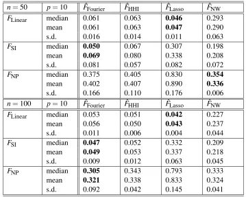
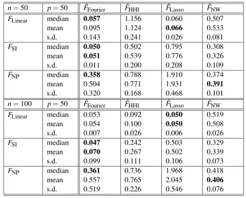
For each experiment, a learning set of sizenwas generated to compute the estimates and their performance, in terms of mean square prevision error, was evaluated on a separate test set of the same size. The results are shown in Table 1 (p=10) and Table 2 (p=50). As each experiment was repeated 20 times, these tables report the median, the mean and the standard deviation (s.d.) of the prevision error of each procedure.

Some comments are in order. First, we note without surprise that:

1. The Lasso performs well in the linear setting [Model 1].

2. The single-index methods ˆFFourier and ˆFHHI are the best ones when the targeted regression

function really involves a single-index model [Model 2].

n=50 p=10 FˆFourier FˆHHI FˆLasso FˆNW

FLinear median 0.061 0.063 0.046 0.293

mean 0.061 0.063 0.047 0.290

s.d. 0.016 0.014 0.011 0.063

F_SI median 0.050 0.067 0.307 0.198

mean 0.069 0.080 0.338 0.208

s.d. 0.081 0.057 0.082 0.072

FNP median 0.375 0.405 0.830 0.354

mean 0.402 0.407 0.890 0.336

s.d. 0.166 0.110 0.176 0.006

n=100 p=10 FˆFourier FˆHHI FˆLasso FˆNW

FLinear median 0.053 0.051 0.042 0.227

mean 0.056 0.050 0.043 0.237

s.d. 0.011 0.006 0.004 0.044

FSI median 0.047 0.052 0.332 0.209

mean 0.049 0.053 0.337 0.218

s.d. 0.009 0.012 0.063 0.045

FNP median 0.305 0.343 0.793 0.333

mean 0.321 0.338 0.833 0.324

s.d. 0.092 0.042 0.145 0.041

Table 1: Numerical results for the simulated data, withn=50 andn=100,p=10. The characters in bold indicate the best performance.

Interestingly, ˆFFourier provides slightly better results than the single-index-tailored estimate ˆFHHI,

especially for p=50. This observation can be easily explained by the fact that ˆFHHI does not

integrate any sparsity information regarding the parameterθ⋆_{, whereas ˆF}

Fouriertries to focus on the

dimension of the active coordinates, which is equal to 2 in this simulation. As a general finding, we retain that ˆFFourier is the most robust of all the tested procedures.

3.3 Real Data

The real-life data sets used in this second series of experiments are from two different sources. The first one, called AIR-QUALITYdata (n=111, p=3), has been first used by Chambers et al. (1983) and has been later considered as a benchmark in the study and comparison of single-index models (see, for example, Antoniadis et al., 2004; Wang, 2009, , among others). This data set originated from an environmental study relatingn=111 ozone concentration measures at p=3 meteorological variables, namely wind speed, temperature and radiation. The data is available as a package in the software R(R Development Core Team, 2008), which we employed in all the numerical experiments. The programs are available upon request from the authors.

The second category of data arises from the UC Irvine Machine Learning Repository http://archive.ics.uci.edu/ml, where the following packages have been downloaded from:

n=50 p=50 FˆFourier FˆHHI FˆLasso FˆNW

FLinear median 0.057 1.156 0.060 0.507

mean 0.095 1.124 0.066 0.533

s.d. 0.143 0.241 0.026 0.081

F_SI median 0.050 0.502 0.795 0.308

mean 0.051 0.539 0.776 0.326

s.d. 0.011 0.200 0.208 0.109

FNP median 0.358 0.788 1.910 0.374

mean 0.504 0.771 1.931 0.391

s.d. 0.320 0.168 0.468 0.101

n=100 p=50 FˆFourier FˆHHI FˆLasso FˆNW

FLinear median 0.053 0.092 0.050 0.519

mean 0.054 0.100 0.050 0.508

s.d. 0.007 0.026 0.006 0.026

FSI median 0.047 0.242 0.503 0.329

mean 0.070 0.267 0.502 0.339

s.d. 0.099 0.111 0.106 0.073

FNP median 0.361 0.736 1.968 0.418

mean 0.557 0.765 2.045 0.406

s.d. 0.519 0.226 0.546 0.076

Table 2: Numerical results for the simulated data, withn=50 andn=100,p=50. The characters in bold indicate the best performance.

• CONCRETE(Yeh, 1998,n=1030,p=8).

• HOUSING(Harrison and Rubinfeld, 1978,n=508,p=13).

• SLUMP-1, SLUMP-2 and SLUMP-3, which correspond to the concrete slump test data introduced by Yeh (2007) (n=51, p=7). Since there are 3 different output variablesY in the original data set, we created a single experiment for each of these variables (1 refers to the output “slump”, 2 to the output “flow” and 3 to the output “28-day Compressive Strength”).

• WINE-REDandWINE-WHITE(Cortez et al., 2009,n=1599,n=4898,p=11). We refer to the above-mentioned references for a precise description of the meaning of the variables involved in these data sets. For homogeneity reasons, all data were normalized to force the input variables to lie in [₋1,1]—in accordance with the setting of our method—and to ensure that all output variables have standard deviation 0.5. In two data sets (AIR-QUALITYandAUTO-MPG) there were some missing values and the corresponding observations were simply removed.

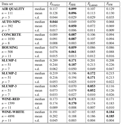
For each method and each of the nine data sets, we randomly split the observations in a learning and a test set of equal sizes, computed the estimate on the learning set, evaluated the prediction error on the test set, and repeated this protocol 20 times. The results are summarized in Table 3.

Data set FˆFourier FˆHHI Fˆ_Lasso FˆNW

AIR QUALITY median 0.117 0.099 0.107 0.129

n=111 mean 0.128 0.096 0.113 0.130

p=3 s.d. 0.044 0.029 0.029 0.035

AUTO-MPG median 0.044 0.049 0.070 0.068

n=392 mean 0.051 0.050 0.072 0.069

p=7 s.d. 0.017 0.006 0.011 0.009

CONCRETE median 0.089 0.087 0.106 0.094

n=1030 mean 0.091 0.087 0.107 0.094

p=8 s.d. 0.008 0.003 0.005 0.004

HOUSING median 0.074 0.059 0.086 0.086

n=508 mean 0.076 0.061 0.085 0.088

p=11 s.d. 0.015 0.013 0.012 0.016

SLUMP-1 median 0.289 0.171 0.201 0.208

n=51 mean 0.244 0.187 0.213 0.226

p=7 s.d. 0.062 0.050 0.049 0.047

SLUMP-2 median 0.219 0.196 0.172 0.215

n=51 mean 0.216 0.194 0.171 0.213

p=7 s.d. 0.053 0.025 0.019 0.022

SLUMP-3 median 0.065 0.070 0.053 0.116

n=51 mean 0.073 0.079 0.052 0.126

p=7 s.d. 0.033 0.027 0.010 0.026

WINE-RED median 0.173 0.171 0.183 0.171

n=1599 mean 0.174 0.170 0.174 0.183

p=11 s.d. 0.009 0.008 0.007 0.010

WINE-WHITE median 0.191 0.187 0.185 0.184

n=4898 mean 0.202 0.188 0.186 0.185

p=11 s.d. 0.045 0.003 0.004 0.004

Table 3: Numerical results for the real-life data sets. The characters in bold indicate the best per-formance.

offers outcomes which are similar to the ones of ˆF_HHI, with a slight advantage for the latter method however. Altogether, ˆFFourierand ˆFHHIprovide the best performance in terms of prediction error in

6 out of 9 experiments. Besides, when it is not the best, the method ˆFFourieris close to the best one,

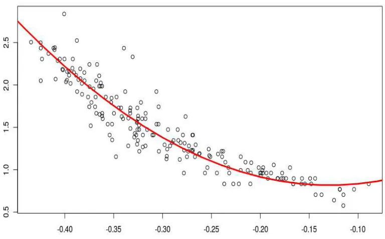
as for example inSLUMP-3andWINE-RED. As an illustrative example, the plot of the resulting fit of our procedure to the data setAUTO-MPGis shown in Figure 1.

Figure 1:AUTO-MPGexample: Estimated link function by the method ˆFFourier.

for sparsity—collapses, whereas ˆFFourier takes a clear advantage over its competitors. In fact, it

provides the best results in 3 out of 9 experiments (AUTO-MPG,CONCRETEandHOUSING). Besides, when it is not the best, the method ˆF_Fourieris very close to the best one, as for example in SLUMP-3andWINE-RED.

Thus, as a general conclusion to this experimental section, we may say that our PAC-Bayesian oriented procedure has an excellent predictive ability, even in nonasymptotic/high-dimensional situ-ations. It is fast, robust, and exhibits performance at the level of the gold standard Lasso. Moreover, as seen in the artificial data analysis, it is expected to perform better than the Lasso if the data cannot be explained approximately by a linear model.

4. Proofs

We start with some preliminary results that will play an important role throughout this section.

4.1 Preliminary Results

Throughout this section, we letπbe the prior probability measure onRp_×

_F

n(C+1)equipped with its canonical Borelσ-field. Recall that

F

n(C+1)⊂

F

and that, for each f ∈

F

n(C+1), we have

Augmented data set FˆFourier FˆHHI Fˆ_Lasso FˆNW

AIR QUALITY median 0.172 0.272 0.164 0.281

n=111 mean 0.244 0.291 0.163 0.291

p=12 s.d. 0.163 0.116 0.038 0.046

AUTO-MPG median 0.043 0.062 0.085 0.202

n=392 mean 0.044 0.072 0.086 0.203

p=28 s.d. 0.009 0.018 0.008 0.014

CONCRETE median 0.087 0.093 0.113 0.245

n=1030 mean 0.087 0.094 0.112 0.094

p=32 s.d. 0.007 0.008 0.005 0.009

HOUSING median 0.071 0.199 0.092 0.226

n=508 mean 0.075 0.181 0.095 0.227

p=44 s.d. 0.023 0.084 0.013 0.018

SLUMP-1 median 0.270 0.426 0.276 0.271

n=51 mean 0.290 0.409 0.274 0.262

p=28 s.d. 0.101 0.079 0.055 0.042

SLUMP-2 median 0.276 0.332 0.195 0.253

n=51 mean 0.285 0.349 0.198 0.254

p=28 s.d. 0.075 0.063 0.043 0.034

SLUMP-3 median 0.079 0.371 0.061 0.372

n=51 mean 0.082 0.361 0.058 0.279

p=28 s.d. 0.025 0.079 0.013 0.031

WINE-RED median 0.178 0.222 0.172 0.245

n=1599 mean 0.176 0.226 0.174 0.246

p=44 s.d. 0.085 0.033 0.006 0.029

WINE-WHITE median 0.199 0.239 0.187 0.252

n=4898 mean 0.204 0.256 0.188 0.260

p=44 s.d. 0.091 0.041 0.005 0.019

Table 4: Numerical results for the real-life data sets augmented with noise variables. The characters in bold indicate the best performance.

Besides, sinceE[Y_|X] = f⋆(θ⋆T_{X)almost surely, we note once and for all that for all(θ,f)∈}

S

_1,+p ×

F

n(C+1),

R(θ,f)₋R(θ⋆,f⋆) =EY₋f(θT_X)2

−EY₋f⋆(θ⋆T_X)2

=Ef(θT_X)−f⋆_(θ⋆T_X)2

Lemma 5 Let T1, . . . ,Tnbe independent real-valued random variables. Assume that there exist two

positive constants v and w such that, for all integers k_≥2,

n

∑

i=1

E

h

(Ti)k+

i

≤k₂!vwk−2.

Then, for anyζ_∈]0,1/w[,

E

"

exp ζ

n

∑

i=1

[Ti−ETi]

!#

≤exp

vζ2

2(1₋wζ)

.

Given a measurable space(E,

E

)and two probability measuresµ1andµ2on(E,

E

), we denote by

K

(µ1,µ2)the Kullback-Leibler divergence ofµ1with respect toµ2, defined by

K

(µ1,µ2) =

 



Z

log

dµ1 dµ2

dµ1 ifµ1≪µ2,

∞ otherwise.

(Notation µ1≪µ2 means “µ1 is absolutely continuous with respect to µ2”.) In the next lemma, notation_◦stands for the function composition operator.

Lemma 6 Let(E,

E

) be a measurable space. For any probability measure µ on (E,

E

)and any

measurable function h:E_→Rsuch thatR(exp_◦h)dµ<∞, we have

log

Z

(exp_◦h)dµ=sup m

Z

hdm₋

K

(m,µ)

, (6)

where the supremum is taken over all probability measures on(E,

E

)and, by convention,∞₋∞=

−∞. Moreover, as soon as h is bounded from above on the support of µ, the supremum with respect

to m on the right-hand side of (6) is reached for the Gibbs distribution g given by

dg

dµ(e) =

exp[h(e)]

Z

(exp_◦h)dµ

, e_∈E.

Lemma 7 Assume that AssumptionNholds. Set w=8(2C+1)max[L,2C+1]and take

λ_∈

0, n

w+ [(2C+1)2_+4σ2_]

.

Then, for all δ_∈]0,1[and any data-dependent probability measure ρˆ absolutely continuous with

respect toπwe have, with probability at least1₋δ,

R(θˆ,fˆ)₋R(θ⋆,f⋆)

≤ 1

1₋λ[(2C_n+1)_−w2_λ+4σ2] Rn

(_θˆ_,fˆ_)−Rn(θ⋆_,f⋆_{) +}log

d ˆρ dπ(θˆ,fˆ)

+log 1_δ

λ

!

,

Proof Fixθ_∈

S

_1,+p and f ∈

F

n(C+1). The proof starts with an application of Lemma 5 to the random variables

Ti=− Yi−f(θTXi)

2

+ Yi−f⋆(θ⋆TXi)

2

, i=1, . . . ,n.

Note that these random variables are independent, identically distributed, and that

n

∑

i=1

ETi2= n

∑

i=1

En

2Yi−f(θTXi)−f⋆(θ⋆TXi)

2

f(θT_X

i)−f⋆(θ⋆TXi)

2o

=

n

∑

i=1

En2Wi+f⋆(θ⋆TXi)−f(θTXi)

2

f(θT_X

i)−f⋆(θ⋆TXi)

2o ≤ n

∑

i=1 E n

4W_i2+ (2C+1)2 f(θTXi)−f⋆(θ⋆TXi)

2o

(sinceE[Wi|Xi] =0).

Thus, by AssumptionN, n

∑

i=1

ET_i2_≤(2C+1)2+4σ2 n

∑

i=1

Ef(θTXi)−f⋆(θ⋆TXi)

2

≤v,

where we set

v=2n[(2C+1)2_+4σ2_{] [R(θ,f)−R(θ}⋆_,f⋆_{)]. (7)}

More generally, for all integersk_≥3,

n

∑

i=1

E

h

(Ti)k+

i ≤ n

∑

i=1 E n

2Y_i−f(θTX_i)−f⋆(θ⋆TX_i)

k

f(θTX_i)−f⋆(θ⋆TX_i) ko = n

∑

i=1 E n

2W_i+f⋆(θ⋆TX_i)−f(θTX_i)

k

f(θTX_i)−f⋆(θ⋆TX_i)

ko

≤2k−1 n

∑

i=1

E

nh

2k_|Wi|k+ (2C+1)k

i

(2C+1)k−2f(θTX_i)−f⋆(θ⋆TX_i)

2o

.

In the last inequality, we used the fact that_|a+b_|k_≤2k−1(_|a_|k+_|b_|k)together with

f(θTX_i)−f⋆(θ⋆TX_i)

k

=f(θTX_i)−f⋆(θ⋆TX_i)

k−2

×f(θTX_i)−f⋆(θ⋆TX_i)

2

≤(2C+1)k−2f(θTX_i)−f⋆(θ⋆TX_i)

Therefore, by AssumptionN, n

∑

i=1

E

h

(Ti)k+

i

≤

n

∑

i=1

h

22k−2k!σ2Lk−2+2k−1(2C+1)ki(2C+1)k−2[R(θ,f)₋R(θ⋆,f⋆)]

=v_×

22k−2k!σ2_Lk−2₊₂k−1_(2C+1)k

(2C+1)k−2 [(2C+1)2_+4σ2_]

≤v_×8

k₋2_{k! max}

Lk−2,(2C+1)k₋2

(2C+1)k₋2 2

=k!

2vw k−2_,

withw=8(2C+1)max[L,2C+1].

Thus, for any inverse temperature parameter λ_∈]0,n/w[, taking ζ=λ/n, we may write by Lemma 5

Enexp[λ(R(θ,f)₋R(θ⋆,f⋆)₋Rn(θ,f) +Rn(θ⋆,f⋆))]

o

≤exp vλ

2 2n2₍₁₋wλ

n )

!

.

Therefore, using the definition ofv, we obtain

E

(

exp

"

λ₋λ 2

(2C+1)2_+4σ2

n(1₋w_nλ)

!

(R(θ,f)₋R(θ⋆,f⋆))

+λ(₋Rn(θ,f) +Rn(θ⋆,f⋆))−log

1 δ

#)

≤δ.

Next, we use a standard PAC-Bayesian approach (Catoni, 2004, 2007; Audibert, 2004; Alquier, 2008). Let us remind the reader thatπis a prior probability measure on the set

S

_1,+p ×

F

n(C+1). We have

Z E

(

exp

"

λ₋λ 2

(2C+1)2_+4σ2

n(1₋w_nλ)

!

(R(θ,f)₋R(θ⋆,f⋆))

+λ(₋Rn(θ,f) +Rn(θ⋆,f⋆))−log

1 δ

#)

dπ(θ,f)_≤δ

and consequently, using Fubini’s theorem,

E

(Z

exp

"

λ₋λ 2

(2C+1)2_+4σ2

n(1₋w_nλ)

!

(R(θ,f)₋R(θ⋆,f⋆))

+λ(₋Rn(θ,f) +Rn(θ⋆,f⋆))−log

1 δ

#

dπ(θ,f)

)

Therefore, for any data-dependent posterior probability measure ˆρabsolutely continuous with re-spect toπ, adopting the convention∞_×0=0,

E

(Z

exp

"

λ₋λ 2

(2C+1)2_+4σ2

n(1₋w_nλ)

!

(R(θ,f)₋R(θ⋆,f⋆))

+λ(₋Rn(θ,f) +Rn(θ⋆,f⋆))

−log

d ˆρ dπ(θ,f)

−log

1 δ

#

d ˆρ(θ,f)

)

≤δ.

Recalling thatP⊗n stands for the distribution of the sample

D

n, the latter inequality can be more conveniently written as

EDn∼P⊗nE(θˆ,fˆ)∼ρˆ

(

exp

"

λ₋λ 2

(2C+1)2_+4σ2

n(1₋w_nλ)

!

R(θˆ,fˆ)₋R(θ⋆,f⋆)

+λ ₋Rn(θˆ,fˆ) +Rn(θ⋆,f⋆)

−log

d ˆρ dπ(θˆ,fˆ)

−log

1 δ

#)

≤δ.

Thus, using the elementary inequality exp(λx)_≥1_R+(x)we obtain, with probability at mostδ,

1₋λ

(2C+1)2_+4σ2

n(1₋w_nλ)

!

R(θˆ,_fˆ_)−R(θ⋆_,f⋆₎

≥Rn(θˆ,fˆ)−Rn(θ⋆,f⋆)

+

log

_dˆ

ρ dπ(θˆ,fˆ)

+log 1_δ

λ ,

where the probability is evaluated with respect to the distributionP⊗n_{of the data}

_D

nandthe condi-tional probability measure ˆρ. Put differently, letting

λ_∈

0, n

w+ [(2C+1)2_+4σ2_]

,

we have, with probability at least 1₋δ,

R(θˆ,fˆ)₋R(θ⋆,f⋆)

≤ 1

1₋λ[(2C_n+1)_−w2_λ+4σ2]

Rn(θˆ,fˆ)−Rn(θ⋆,f⋆) +

log

_d

ˆ ρ dπ(θˆ,fˆ)

+log 1_δ λ

!

.

Lemma 8 Under the conditions of Lemma 7 we have, with probability at least1₋δ, Z

Rn(θ,f)d ˆρ(θ,f)−Rn(θ⋆,f⋆)

≤ 1+λ

(2C+1)2_+4σ2

n₋wλ

! Z

R(θ,f)d ˆρ(θ,f)₋R(θ⋆,f⋆)

+

K

(ρˆ,π) +log 1 δ

λ .

Proof The beginning of the proof is similar to the one of Lemma 7. More precisely, we apply Lemma 5 with Ti = (Yi−f(θTXi))2−(Yi−f⋆(θ⋆TXi))2 and obtain, for any inverse temperature parameterλ_∈]0,n/w[,

Enexp[λ(R(θ⋆,f⋆)₋R(θ,f)₋Rn(θ⋆,f⋆) +Rn(θ,f))]

o

≤exp vλ

2 2n2₍₁₋wλ

n )

!

(see (7) for the definition ofv). Thus, using the definition ofv,

E

(

exp

"

λ+λ 2

(2C+1)2_+4σ2

n(1₋w_nλ)

!

(R(θ⋆,f⋆)₋R(θ,f))

+λ(Rn(θ,f)−Rn(θ⋆,f⋆))−log

1 δ

#)

≤δ.

Integrating with respect toπleads to

Z E

(

exp

"

λ+λ 2

(2C+1)2_+4σ2

n(1₋w_nλ)

!

(R(θ⋆,f⋆)₋R(θ,f))

+λ(Rn(θ,f)−Rn(θ⋆,f⋆))−log

1 δ

#)

dπ(θ,f)_≤δ

whence, by Fubini’s theorem,

E

(Z

exp

"

λ+λ 2

(2C+1)2_+4σ2

n(1₋w_nλ)

!

(R(θ⋆,f⋆)₋R(θ,f))

+λ(Rn(θ,f)−Rn(θ⋆,f⋆))−log

1 δ

#

dπ(θ,f)

)

≤δ.

Thus, for any data-dependent posterior probability measure ˆρabsolutely continuous with respect to π,

E

(Z

exp

"

λ+λ 2

(2C+1)2_+4σ2

n(1₋w_nλ)

!

(R(θ⋆,f⋆)₋R(θ,f))

+λ(Rn(θ,f)−Rn(θ⋆,f⋆))

−log

d ˆρ dπ(θ,f)

−log 1 δ #

d ˆρ(θ,f)

)

Therefore, by Jensen’s inequality,

E

(

exp

Z "

λ+λ 2

(2C+1)2_+4σ2

n(1₋w_nλ)

!

(R(θ⋆,f⋆)₋R(θ,f))

+λ(Rn(θ,f)−Rn(θ⋆,f⋆))

−log

d ˆρ dπ(θ,f)

−log

1 δ

#

d ˆρ(θ,f)

)

=E

(

exp

"

λ+λ 2

(2C+1)2_+4σ2

n(1₋w_nλ)

!

R(θ⋆,f⋆)₋

Z

R(θ,f)d ˆρ(θ,f)

+λ

Z

Rn(θ,f)d ˆρ(θ,f)−Rn(θ⋆,f⋆)

−

K

(ρˆ,π)₋log

1 δ

#)

≤δ.

Consequently, by the elementary inequality exp(λx)_≥1_R+(x), we obtain, with probability at most δ,

Z

Rn(θ,f)d ˆρ(θ,f)−Rn(θ⋆,f⋆)

≥ 1+λ

(2C+1)2_+4σ2

n−wλ

! Z

R(θ,f)d ˆρ(θ,f)₋R(θ⋆,f⋆)

+

K

(ρˆ,π) +log 1 δ

λ .

Equivalently, with probability at least 1₋δ,

Z

Rn(θ,f)d ˆρ(θ,f)−Rn(θ⋆,f⋆)

≤ 1+λ

(2C+1)2_+4σ2

n₋wλ

! Z

R(θ,f)d ˆρ(θ,f)₋R(θ⋆,f⋆)

+

K

(ρˆ,π) +log 1 δ

4.2 Proof of Theorem 2

The proof starts with an application of Lemma 7 with ˆρ=ρˆ_λ(the Gibbs distribution) as posterior distribution. More precisely, we know that, with probability larger than 1₋δ,

R(θˆ_λ,_fˆ_λ)−R(θ⋆_,f⋆_)≤ 1

1₋λ[(2C_n+1)_−w2_λ+4σ2]

Rn(θˆλ,fˆλ)−Rn(θ⋆,f⋆)

+

log

_dˆ

ρλ

dπ(θˆλ,fˆλ)

+log 1_δ λ

!

,

where the probability is evaluated with respect to the distributionP⊗n_{of the data}

_D

nandthe condi-tional probability measure ˆρλ. Observe that

log

d ˆρ_λ

dπ(θˆλ,fˆλ)

=log



 

exp

−λRn(θˆλ,fˆλ)

Z

exp[₋λRn(θ,f)]dπ(θ,f)



 

=₋λRn(θˆλ,fˆλ)−log

Z

exp[₋λRn(θ,f)]dπ(θ,f).

Consequently, with probability at least 1₋δ,

R(θˆλ,fˆλ)−R(θ⋆,f⋆)≤

1

λ1₋λ[(2C_n+1)_−w2_λ+4σ2]

−log

Z

exp[₋λRn(θ,f)]dπ(θ,f)

−λRn(θ⋆,f⋆) +log

1 δ

!

.

Next, using Lemma 6 we deduce that, with probability at least 1₋δ,

R(θˆλ,fˆλ)−R(θ⋆,f⋆)≤

1

1₋λ[(2C_n+1)_−w2_λ+4σ2] inf

ˆ ρ

(Z

Rn(θ,f)d ˆρ(θ,f)−Rn(θ⋆,f⋆)

+

K

(ρˆ,π) +log 1 δ

λ

)

,

where the infimum is taken over all probability measures on

S

_1,+p ×

F

n(C+1). In particular, letting

M

(I,M)be the set of all probability measures on

S

_1,+p (I)_×

F

M(C+1), we have, with probability at least 1₋δ,

R(θˆλ,fˆλ)−R(θ⋆,f⋆)

≤ 1

1₋λ[(2C_n+1)_−w2_λ+4σ2] I⊂ {inf1, . . . ,p}

1≤M≤n

inf ˆ ρ∈M(I,M)

(Z

Rn(θ,f)d ˆρ(θ,f)−Rn(θ⋆,f⋆)

+

K

(ρˆ,π) +log 1 δ

λ

)

Next, observe that, for ˆρ_∈

M

(I,M),

K

(ρˆ,π) =

K

(ρˆ,µ⊗ν) =

K

(ρˆ,µI⊗νM) +log





1_{− 10}1p

1_{− 10}1n p |I_|

10−|I|−M





≤

K

(ρˆ,µI⊗νM) +log

" p |I|

10−|I|−M

#

. (8)

Therefore, with probability at least 1₋δ,

R(_θˆ_λ,fˆ_λ)−R(θ⋆_,f⋆₎

≤ 1

1₋λ[(2C_n+1)_−w2_λ+4σ2] inf I⊂ {1, . . . ,p}

1≤M≤n

inf ˆ

ρ∈M(I,M)

(Z

Rn(θ,f)d ˆρ(θ,f)−Rn(θ⋆,f⋆)

+

K

(ρˆ,µI⊗νM) +log

(p |I|) 10−|I|−M

+log 1_δ λ

)

. (9)

By Lemma 8 and inequality (8), for any data-dependent distribution ˆρ_∈

M

(I,M), with probability at least 1₋δ,

Z

Rn(θ,f)d ˆρ(θ,f)−Rn(θ⋆,f⋆)

≤ 1+λ

(2C+1)2_+4σ2

n₋wλ

! Z

R(θ,f)d ˆρ(θ,f)₋R(θ⋆,f⋆)

+

K

(ρˆ,µI⊗νM) +log

(p |I|) 10−|I|−M

+log 1_δ

λ . (10)

Thus, combining inequalities (9) and (10), we may write, with probability at least 1₋2δ,

R(θˆ_λ,_fˆ_λ)−R(θ⋆_,f⋆₎

≤ 1

1₋λ[(2C_n+1)_−w2_λ+4σ2] inf I⊂ {1, . . . ,p}

1≤M≤n

inf ˆ

ρ∈M(I,M)

(

1+λ

(2C+1)2_+4σ2

n₋wλ

! Z

R(θ,f)d ˆρ(θ,f)₋R(θ⋆,f⋆)

+2

K

(ρˆ,µI⊗νM) +log

(p |I|) 10−|I|−M

+log 1_δ λ

)

. (11)

For any subsetI of_{1, . . . ,p_}, any positive integerM_≤nand anyη,γ_∈]0,1/n], let the probability measureρI,M,η,γbe defined by

with

dρ1

I,M,η dµI

(θ)∝1_[kθ−θ⋆ I,Mk1≤η]

and

dρ2

I,M,γ dνM

(f)∝1_[kf−f⋆ I,MkM≤γ]

where, for f=∑Mj=1βjϕj∈

F

M(C+1), we put

kf_kM= M

∑

j=1

j_|βj|.

With this notation, inequality (11) leads to

R(θˆ_λ,fˆλ)−R(θ⋆,f⋆)

≤ 1

1₋λ[(2C_n+1)_−w2_λ+4σ2] inf I⊂ {1, . . . ,p}

1≤M≤n inf η,γ>0

(

1+λ

(2C+1)2_+4σ2

n₋wλ

! Z

R(θ,f)dρI,M,η,γ(θ,f)−R(θ⋆,f⋆)

!

+2

K

(ρI,M,η,γ,µI⊗νM) +log

(p |I|) 10−|I|−M

+log 1_δ λ

)

. (12)

To finish the proof, we have to control the different terms in (12). Note first that

log

p |I_|

≤ |I_|log

pe |I_|

and, consequently,

log

" p |I|

10−|I|−M

#

≤ |I_|log

pe |I_|

+ (_|I_|+M)log 10. (13)

Next,

K

(ρI,M,η,γ,µI⊗νM) =

K

(ρ1I,M,η⊗ρ2I,M,γ,µI⊗νM)

=

K

(ρ1

I,M,η,µI) +

K

(ρ2I,M,γ,νM). By technical Lemma 9, we know that

K

(ρ1_I,M,η,µI)≤(|I| −1)log

max

|I_|,4 η

.

Similarly, by technical Lemma 10,

K

(ρ2

I,M,γ,νM) =Mlog

C+1

γ

Putting all the pieces together, we are led to

K

(ρI,M,η,γ,µI⊗νM)≤(|I| −1)log

max

|I_|,4 η

+Mlog

C+1

γ

. (14)

Finally, it remains to control the term

Z

R(θ,f)dρI,M,η,γ(θ,f).

To this aim, we write

Z

R(θ,f)dρI,M,η,γ(θ,f)

=

Z E

h

Y₋f(θTX)2i

dρI,M,η,γ(θ,f)

=

Z

E Y₋f_I⋆_,M(θ⋆T

I,MX) +fI⋆,M(θI⋆,TMX)−f(θ⋆I,TMX)

+f(θ⋆_I,T_MX)₋f(θTX)2

dρI,M,η,γ(θ,f)

=R(θ⋆_I,M,f_I⋆_,M)

+

Z E

h

f_I⋆_,M(θ⋆T

I,MX)−f(θ⋆I,TMX)

2

+ f(θ⋆T

I,MX)−f(θTX)

2

+2 Y−f_I⋆_,M(θ⋆T I,MX)

f_I⋆_,M(θ⋆T

I,MX)−f(θ⋆I,TMX)

+2 Y₋f_I⋆_,M(θ⋆T I,MX)

f(θ⋆T

I,MX)−f(θTX)

+2 f_I⋆_,M(θ⋆T

I,MX)−f(θ⋆I,TMX)

f(θ⋆T

I,MX)−f(θTX)

i

dρI,M,η,γ(θ,f)

:=R(θ⋆_I,M,f_I⋆_,M) +A+B+C+D+E.

4.2.1 COMPUTATION OFC

By Fubini’s theorem,

C=E

Z

2 Y₋f_I⋆_,M(θ⋆T I,MX)

f_I⋆_,M(θ⋆T

I,MX)−f(θ⋆I,TMX)

dρI,M,η,γ(θ,f)

=E

(Z "

2 Y₋f_I⋆_,M(θ⋆T I,MX)

× Z

f_I⋆_,M(θ⋆_I,T_MX)₋f(θ⋆_I,T_MX)

dρ2_I,M,γ(f)

#

dρ1_I,M,η(θ)

)

.

By the triangle inequality, for f=∑Mj=1βjϕj and fI⋆,M=∑Mj=1(β⋆I,M)jϕj, it holds

M

∑

j=1

j_|βj| ≤

M

∑

j=1

jβ_j−(β⋆_I,M)_j

+

M

∑

j=1

Since f_I⋆_,M ∈

F

M(C), we have ∑Mj=1j|(βI⋆,M)j| ≤C, so that ∑Mj=1j|βj| ≤C+1 as soon as kf−

f_I⋆_,MkM≤1. This shows that the set

(

f =

M

∑

j=1

βjϕj:kf−fI⋆,MkM≤γ

)

is contained in the support of νM. In particular, this implies that ρ2I,M,γ is centered at fI⋆,M and, consequently,

Z

f_I⋆_,M(θ⋆T

I,MX)−f(θ⋆I,TMX)

dρ2

I,M,γ(f) =0.

This proves thatC=0.

4.2.2 CONTROL OFA

Clearly,

A_≤

Z

sup y∈R

(f_I⋆_,M(y)₋f(y)2

dρ2

I,M,γ(f)≤γ2.

4.2.3 CONTROL OFB

We have

B=

Z

Eh f(θ⋆T

I,MX)−f(θTX)

2i

dρI,M,η,γ(θ,f)

≤ Z

E

h

ℓ(C+1)(θ_I⋆_,T_M−θT)X2

i

dρ1_I,M,η(θ) (by the mean value theorem)

≤ℓ2(C+1)2EkX_k2_∞

Z

kθ⋆_I,M−θ_k2₁dρ1_I,M,η(θ)

4.2.4 CONTROL OFE

Write

|E_{| ≤}2

Z

Ehf_I⋆_,M(θ_I⋆_,T_MX)−f(θ⋆_I,T_MX)

×

f(θ⋆_I,T_MX)−f(θTX) i

dρI,M,η,γ(θ,f)

≤2

Z

Ehf_I⋆_,M(θ_I⋆_,T_MX)−f(θ⋆_I,T_MX)

×ℓ(C+1)

(θ⋆_I,T_M−θT)X i

dρI,M,η,γ(θ,f)

≤2

Z

E

h

f_I⋆_,M(θ⋆_I,T_MX)₋f(θ⋆_I,T_MX)2i

dρI,M,η,γ(θ,f)

1₂

Z

E

h

ℓ(C+1)(θ⋆T

I,M−θT)X

2i

dρI,M,η,γ(θ,f)

1₂

(by the Cauchy-Schwarz inequality)

≤2 γ21₂

ℓ2(C+1)2η21₂

=2ℓ(C+1)γη.

4.2.5 CONTROL OFD

Finally,

D=2

Z

E

Y−f_I⋆_,M(θ⋆T

I,MX)

f(θ⋆T

I,MX)−f(θTX)

dρI,M,η,γ(θ,f)

=2

Z

E Y₋f_I⋆_,M(θ⋆_I,T_MX)

f_I⋆_,M(θ⋆_I,T_MX)₋f_I⋆_,M(θTX)

dρ1_I,M,η(θ) (since

Z

fdρ2_I,M,γ(f) = f_I⋆_,M)

=2E

Y₋f_I⋆_,M(θ⋆T

I,MX)

Z

f_I⋆_,M(θ⋆T

I,MX)−fI⋆,M(θTX)

dρ1

I,M,η(θ)

≤2 s E

Y₋f_I⋆_,M(θ⋆T

I,MX)

2 × s E Z

f_I⋆_,M(θ⋆T

I,MX)−fI⋆,M(θTX)

dρ1

I,M,η(θ)

2

(by the Cauchy-Schwarz inequality)

=2qR(θ⋆

I,M,fI⋆,M)

s

E

Z

f_I⋆_,M(θ⋆T

I,MX)−fI⋆,M(θTX)

dρ1

I,M,η(θ)

2

.

The inequality

f_I⋆_,M(θ⋆_I,T_MX)−f_I⋆_,M(θTX)

≤ℓ(C+1)

(θ⋆_I,T_M−θT)X

leads to

Z

f_I⋆_,M(θ⋆T

I,MX)−fI⋆,M(θTX)

dρ1

I,M,η(θ)

2

≤ℓ2(C+1)2

Z

kθ⋆_I,M−θ_k1dρ1I,M,η(θ)

2

.

Consequently,

Z

f_I⋆_,M(θ⋆_I,T_MX)₋f_I⋆_,M(θTX)

dρ1_I,M,η(θ)

2

≤ℓ2(C+1)2η2,

and therefore

D_≤2ℓ(C+1)ηpR(0,0)/2

≤√2ℓ(C+1)ηpC2_+σ2_. Thus, takingη=γ=1/nand putting all the pieces together, we obtain

A+B+C+D+E_≤Ξ1

n ,

whereΞ1is a positive constant, depending onC,σandℓ. Combining this inequality with (12)-(14) yields, with probability larger than 1₋2δ,

R(θˆλ,fˆλ)−R(θ⋆,f⋆)

≤ 1

1₋λ[(2C_n+1)_−w2_λ+4σ2] I⊂ {inf1, . . . ,p}

1≤M≤n

(

1+λ

(2C+1)2_+4σ2

n₋wλ

!

R(θ⋆_I,M,f_I⋆_,M)

−R(θ⋆,f⋆) +Ξ1

n

!

+2Mlog(10(C+1)n) +|I|log(40epn) +log 1 δ

λ

)

.

Choosing finally

λ= n

w+2[(2C+1)2_+4σ2_],

we obtain that there exists a positive constantΞ2, function ofL,C,σandℓsuch that, with probability at least 1₋2δ,

R(θˆ_λ,fˆλ)−R(θ⋆,f⋆)≤Ξ2 inf

I⊂ {1, . . . ,p}

1≤M≤n

(

R(θ⋆_I,M,f_I⋆_,M)₋R(θ⋆,f⋆)

+Mlog(10Cn) +|I|log(40epn) +log 1 δ

n

)

.