R E S E A R C H A R T I C L E
Open Access
Meta-analysis of binary outcomes via
generalized linear mixed models: a simulation
study
Ilyas Bakbergenuly
*and Elena Kulinskaya
Abstract
Background: Systematic reviews and meta-analyses of binary outcomes are widespread in all areas of application. The odds ratio, in particular, is by far the most popular effect measure. However, the standard meta-analysis of odds ratios using a random-effects model has a number of potential problems. An attractive alternative approach for the meta-analysis of binary outcomes uses a class of generalized linear mixed models (GLMMs). GLMMs are believed to overcome the problems of the standard random-effects model because they use a correct binomial-normal
likelihood. However, this belief is based on theoretical considerations, and no sufficient simulations have assessed the performance of GLMMs in meta-analysis. This gap may be due to the computational complexity of these models and the resulting considerable time requirements.
Methods: The present study is the first to provide extensive simulations on the performance of four GLMM methods (models with fixed and random study effects and two conditional methods) for meta-analysis of odds ratios in comparison to the standard random effects model.
Results: In our simulations, the hypergeometric-normal model provided less biased estimation of the heterogeneity variance than the standard random-effects meta-analysis using the restricted maximum likelihood (REML) estimation when the data were sparse, but the REML method performed similarly for the point estimation of the odds ratio, and better for the interval estimation.
Conclusions: It is difficult to recommend the use of GLMMs in the practice of meta-analysis. The problem of finding uniformly good methods of the meta-analysis for binary outcomes is still open.
Keywords: Generalized linear mixed-effects models, Random effects, Hypergeometric-normal likelihood, Transformation bias, Meta-analysis
Background
Meta-analysis is a statistical technique for synthesiz-ing outcomes from several studies. Since the individ-ual studies might differ in populations and structure [1, 2], their effects are often assumed to be heteroge-neous, and the use of methods based on random-effects models is recommended. When the outcome of interest is a transformation of a binomial outcome such as the logit transformation, the standard random-effects model assumes that within-study variability can be described by an approximate normal likelihood, i.e. the estimates
*Correspondence:[email protected]
School of Computing Sciences, University of East Anglia, NR4 7TJ Norwich, UK
of effects θˆi ∼ Nθi,σi2 in each study i, i = 1. . .,K. Combining this assumption with a normal distribution of
true effects between studies, θi ∼ Nθ,τ2, the
result-ing marginal random-effects model isθˆi ∼N
θ,σi2+τ2. However, the standard REM has several potential prob-lems. It makes the strong assumption that the estimated
within-study variances σˆi2 can be used in place of the
unknown true variancesσi2(without accounting for their
variability), and it does not account for the correlation
between the estimated within-study variancesσˆi2and the
effect measuresθˆi [3–5]. Additionally, the standard REM
suffers from transformation bias ([6]) and bias in the
estimation of the random-effect varianceτ2.
An attractive alternative approach for the meta-analysis of binary outcomes uses a class of generalized linear mixed models (GLMMs). These models can be fitted in
SAS [3] and in R using themetaforpackage by Viechtbauer
[7]. Generalized linear mixed models are believed to over-come the problems of the standard random-effects model [3] because they use a binomial-normal likelihood. How-ever, this belief is based on theoretical considerations, and no sufficient simulations have assessed the performance of methods based on GLMMs in meta-analysis. This gap may be due to the computational complexity of these models and the resulting considerable time requirements for simulations.
We concentrate on the meta-analysis of odds ratios (OR), by far the most popular effect measure, with
normally-distributed true effects θi between studies.
Other mixing distributions for random effects are possible [8]. A natural alternative is a beta-binomial model, which assumes a beta mixing distribution for the event proba-bilities. This model was recommended for use with sparse data by Kuss [9] and studied in much detail in [10].
The relative risk (RR) is often a more appropriate measure of effect than the odds ratio, and it has a direct interpretation. Reasons for choosing RR instead of OR and the ease with which OR can be misinterpreted are discussed in [11–15]. However, perhaps due to the math-ematical convenience and to the widely available software implementations, the odds ratio is by far the most popular effect measure.
Our simulations have used all four GLMM methods
available inmetafor: GLMM with fixed or random study
effects [16]; the noncentral-hypergeometric-normal
model (NCHGN) discussed by Van Houwelingen et al. [17], Liu and Pierce [18], Sidik and Jonkman [19] and Stijnen et al. [3]; and an approximation of noncentral-hypergeometric-normal model by a binomial-normal
model, method CM.AL in metafor. For comparison, we
also included two standard inverse-variance weights based methods, DerSimonian-Laird (DL) [20] and restricted maximum likelihood (REML), routinely used in random-effects meta-analysis.
Among the GLMMs available for the meta-analysis of binary outcomes, we are particularly interested in the NCHGN. The exact distribution for the number of events conditional on marginal totals is the noncentral hyperge-ometric distribution. The NCHGN model also includes a normally distributed random effect (log odds ratio) for studies. However, the performance of this model is not well known. The simulation study on GLMMs in meta-analysis by Kuss [9] compared several methods for
analysing sparse 2× 2 data but excluded the NCHGN
model and its approximation by the binomial-normal dis-tribution as they exclude double-zero studies, i.e. studies with zero events in both arms. The recent simulation
study by Jackson et al. [21] examined the use of seven GLMMs for summary odds ratio, including the NCHGN model and the other models considered in our study. However, Jackson et al. [21] considered only 15 config-urations of the parameters, limited almost exclusively to
K = 10 studies, the baseline probability of 0.2 and the
small value ofτ2 = 0.024. We provide extensive
simula-tions for 880 configurasimula-tions of the parameters, including
K = 3, 5, 10 and 30 studies, the baseline probabilities
from 0.1 to 0.4, and the heterogeneity varianceτ2from 0
to 1. The span of our simulations is instrumental in detect-ing important trends in performance of GLMMs for the meta-analysis of odds ratios.
Our simulation results demonstrate that the GLMM models including the NCHGN do not outperform the standard DL and REML methods in point and interval estimation of overall effect measure. Possible reasons to the unexpected inferior performance of GLMM methods are pointed out in the discussion. The structure of the rest of this paper is as follows.
“Methods” section reviews the GLMMs for binary out-comes and discusses likelihood-based models for log odds ratio. It also describes the simulation study. “Results” section presents the results of simulations and provides an illustrative example. “Discussion” section summa-rizes our results. “Conclusions” section provides further recommendations.
Methods
General formulation of generalized linear mixed models for meta-analysis of binary outcomes
The generalized linear mixed effects model (GLMM) extends the generalized linear model by including random effects in addition to fixed effects (hence mixed-effects model). The inference in GLMMs is based on the likeli-hood.
For the general case, let the univariate observation in
the ith study beyi, and the vectors of covariates xi and
zi of dimensions p and q stand for fixed and random
effects, respectively, for i = 1,. . .,K. The responses yi
are assumed to be independent with conditional means E(yi|bi)=μi(bi)and variances Var(yi|bi)=aiυ(μi(bi)),
whereis the dispersion parameter,aiis a known
con-stant,biis a random effect andυ(·)is a variance function
[22]. The conditional mean and variance have a mean-variance relation, and both of them depend on a
ran-dom effectbi. Given the q-dimensional vector of random
effectsb, the generalized linear mixed model has the form
ηib(b)=xitβ+ztib, (1)
where β is the vector of regression parameters and tis
Inverting the link function,H = g−1, and denoting the
design matrices with rows xti and zti by X and Z, the
conditional mean satisfies
E(y|b)=H(Xβ+Zb),
where y = (y1,. . .,yK). The random effect b follows a
(usually multivariate normal) distribution with zero mean
and with variance-covariance matrixD = D(ζ ), for an
unknown vector of variance componentsζ. Breslow and
Clayton [22] consider models with binomial, Poisson, and hypergeometric specifications for the conditional
distri-bution ofyi and the dispersion parameter = 1 in the
conditional variance. The value of >1 is often used to
model overdispersion, andis estimated jointly with the
parametersζ inD=D(ζ ).
In generalized linear mixed models, the parame-ters are estimated by maximum likelihood. However, because of nonlinearity of the model and the pres-ence of random effects, the marginal distribution for the maximum-likelihood approach includes a cumber-some integration with respect to unobservable ran-dom effects. Usually, the integration does not have a closed form, and therefore no analytic solution is possible. Numerical methods such as adaptive Her-mite quadrature (GHQ) and Laplace’s method have to be applied to evaluate the integral, approximation of the log-likelihood function, score equations, and infor-mation matrix [22]. Alternative estiinfor-mation techniques include penalized quasi-likelihood method (PQL) [22], equivalent pseudo-likelihood method, and higher order Laplace approximations, see [23] for review. Alter-natively, a Bayesian approach uses stochastic inte-gration by Markov chain Monte Carlo (MCMC) or Gibbs sampling to fit GLMMs. Hybrid methods are also available [24]. The moment-based generalized esti-mation equation (GEE) method can also be used for population-average parameter estimation in the marginal models.
GLMMs for the meta-analysis of odds ratios
For binary outcomes yi and the logit link functiong(·),
the model (1) is a logistic regression model with random effects. In a meta-analysis, the study effects correspond to the intercept, and the treatment effect to the slope of treatment/control indicator in the logistic regression; the log odds ratio (LOR) is the difference between the log odds of the treatment and control groups. Platt et al. [25] and Gao [26] considered a generalized linear mixed model with a fixed treatment effect and a random intercept term for each study and provided some simulations on the use of a PQL, GHQ and a linear model fitted by weighted least squares. The use of this model for sparse data was further studied in the extensive simulation study by Kuss [9], who compared a large number of available fitting
methods including a PQL, GHQ, MCMC, beta-binomial model, GEE, and conditional logistic regression. However, GLMMs with random treatment effect are more tradi-tional in meta-analysis. These models may include fixed intercepts (study effects) and random treatment effect, or both intercept and treatment effect are assumed to be random [16].
In the meta-analysis of binary outcomes, the distri-butions of the fixed effects are based on a binomial or noncentral hypergeometric distribution, and the random effects are assumed to follow normal distribution, result-ing in a binomial-normal or hypergeometric-normal like-lihood, respectively. The standard REM is based on the normal approximation to the distribution of log-odds, this is the normal-normal model. For incidence rates, an example of a GLMM is the Poisson-normal model.
Turner et al. [16] introduced a mixed effects logistic regression model with random treatment effect as a mul-tilevel model for meta-analysis of binary outcomes in a frequentist setting. Stijnen et al. [3] proposed to use a con-ditional logistic model with an exact noncentral hyperge-ometric distribution and its approximation by a binomial distribution. The difference between the standard random effects model and a mixed effects logistic regression is that the standard random effects model directly models an effect measure that reflects the contrast between the two groups (e.g., log odds ratio). The conditional logis-tic (hypergeometric) model deals with the OR directly as the study effects are conditioned out. The parameters in these models can be estimated by maximum likelihood or restricted maximum likelihood methods using iterative generalized least squares.
Standard inverse-variance random effects model for the meta-analysis of binary outcomes (REM)
Consider K comparative studies reporting summary
binary outcomes. The data from each studyi = 1,· · ·,K
constitutes a pair of independent binomial variables yi1
andyi2, numbers of events out ofni1andni2subjects for
the treatment and control arms. The risks in the
treat-ment and the control arms are denoted byπijforj=1, 2,
respectively. The log odds ratio for individual studyi is
θi=log(πi1(1−πi2)/(πi2(1−πi1))).
The standard REM is a two-level model. At the first
level, conditionally on the study effectsθi, empirical LORs
ˆ
θi are assumed to be normally distributed with unknown
meansθiand within-study variancesσi2,θˆi ∼ Nθi,σi2. The variances σi2 =[ni1πi1(1 − πi1)]−1+[ni2πi2(1 −
πi2)]−1 are estimated from the data, but their estimates
ˆ
σi2 are assumed to be known. At the second level, the
true within-study effects θi are assumed to have a
nor-mal distribution with meanθand unknown between study
variance τ2, i.e. θi ∼ N
θ,τ2, where θ is the overall
ˆ
θi = θ + νi + i with νi ∼ N
0,τ2, i ∼ N
0,σi2
and Cov(νi,i) = 0. The between-study variance τ2 is
usually estimated by DL [20] or REML, and the overall
LOR θ is estimated using the inverse variance weights
wi=
ˆ
σi2+ ˆτ2−1asθˆ=wiθˆi/
wi.
GLMMs with fixed intercept (FIM)
GLMM with fixed intercept is a special case of mixed effects logistic regression model [16]. The model also accounts for heterogeneity between studies on the log odds scale. The model is written as:
yij|πij∼Binomial(nij,πij) j=1, 2; i=1,. . .,K,
log
πij 1−πij
=φi+(θ+vi)xij, (2)
whereπijare the probabilities of an event in each arm,θis
the overall effect (log odds ratio), and the random effects vi∼N
0,τ2are the deviations of theithstudy treatment
effect (log odds ratio) from the overall effectθ, with τ2
being the between-study variance. The fixed interceptsφi
are the log-odds in the control arms. Thexijis the group
dummy variable. Whenxij = 0/1, then model (2) can be
written as:
log
πi1 1−πi1
=φi+θ+vi and log
πi2 1−πi2
=φi,
for the treatment and control groups, respectively, so that ⎛
⎝log
πi2 1−πi2
log πi1
1−πi1
⎞
⎠∼N
φi φi+θ
,
0 0
0 τ2
. (3)
We will refer to this model as FIM1.
This model assumes higher variability in the treatment
groups. In order to avoid this asymmetry, a coding of+1/2
and−1/2 was suggested for the group dummyxijin [16].
Whenxij = ±1/2 and after reparametrizationφi∗= φi−
θ/2, the model (2) can be written as:
log
πi1 1−πi1
=φi∗+θ+0.5vi and
log
πi2 1−πi2
=φi∗−0.5vi,
for the treatment and control groups, so that ⎛
⎝log 1−πi2πi2
log πi1
1−πi1
⎞
⎠∼N
φi∗ φi∗+θ
,
τ2/4 −τ2/4 −τ2/4 τ2/4
.
(4)
We will refer to this model as FIM2. In [21], the models FIM1 and FIM2 are referred to as models 2 and 4, respectively. They are logistic regression models with
φi = log(πi2/(1−πi2))as the study-specific fixed
inter-cepts that have to be estimated. The unknown
parame-tersφi,θ andτ2are estimated iteratively using marginal
quasi-likelihood, penalized quasi-likelihood, or first- and second-order Taylor-expansion approximation. In order to remove the bias of the between-study variance esti-mates from penalized quasi-likelihood methods, a two-step bootstrap procedure can be used [16]. Jackson et al. [21] demonstrated in simulations and provided a theoret-ical explanation for the inferiority of FIM1 in comparison to FIM2 in respect to considerable underestimation of the
heterogeneity varianceτ2. We further study FIM2 but not
FIM1 in our simulations.
GLMMs with random intercept (RIM)
A GLMM with a random intercept is a mixed effects logis-tic regression model with a random intercept and random treatment effect [16]. The model can be written as:
yij∼Binomial(nij,πij); j=1, 2, i=1,. . .,K,
log
π
ij 1−πij
=φ+ui+(θ+vi)xij, (5)
where φ is the baseline log-odds,θ is the overall effect
(log-odds-ratio), the random effects are random variables
from a bivariate normal distributionvi ∼ N
0,τ2,ui ∼
N0,σ2and Cov(ui,vi) = ωσ τ. This general bivariate
normal random effects model was introduced in [17] and
further discussed in [3]. Whenxij = 0/1, and assuming
Cov(ui,vi)=0, the model (5) can be written as:
log
πi1 1−πi1
=φ+ui+θ+vi and log
πi2 1−πi2
=φ+ui,
so that ⎛
⎝log 1−πi2πi2
log πi1
1−πi1
⎞
⎠∼N
φ φ+θ
,
σ2 σ2 σ2 σ2+τ2
.
(6)
We will refer to this model as RIM1.
Similarly to FIM2, when xij = ±1/2 and assuming
Cov(ui,vi)=0, model (5) can be reparametrized as:
log
πi1 1−πi1
=φ∗+ui+θ+0.5vi and
log
πi2 1−πi2
=φ∗+ui−0.5vi,
for the treatment and control groups, so that ⎛
⎝log 1−πi2πi2
log πi1
1−πi1
⎞ ⎠∼N
φ∗ φ∗+θ
,
σ2+τ2/4 σ2−τ2/4 σ2−τ2/4 σ2+τ2/4
.
(7)
We will refer to this model as RIM2.
The RIM models include two or three (when ω =
Cov(ui,vi) =0) heterogeneity parameters
σ2, τ2, ωin contrast to the standard random effects model with a
φ,θ, σ2,τ2andωcan be estimated similarly to estima-tion in a GLMM with fixed study effects [16]. In [21], the models RIM1 and RIM2 are referred to as models 3 and 5, respectively, and appear to have very similar proper-ties, whereas our general model (5) is their Model 6. The properties of a logistic regression model with a random intercept for the meta-analysis of proportions were also studied by Hamza et al. [27], and for the case of scarce data by Kuss [9]. We further study RIM2 in our simulations.
A GLMM with exact noncentral hypergeometric-normal likelihood (NCHGN)
The hypergeometric-normal model was initially proposed for meta-analysis by Van Houwelingen et al. [17] and Liu and Pierce [18]. Later, Stijnen et al. [3] and Sidik and Jonkman [19] implemented the model. Some simulation results are given in [21], their model 7.
The data may be generated from either FIM or RIM.
Conditioning on the total number of events for studyi,
only the number of events in the treatment groupyi1is
random. NCHGN is a two-level model. Given the
study-specific log odds ratio θi, the distribution of yi1 is the
noncentral hypergeometric distribution. Next, the LORs
θiare normally distributedθi ∼N
θ,τ2. The exact
like-lihood function of the hypergeometric-normal model for
studyican be written as:
hyi1;θ,τ2
=
∞
−∞f(yi1|θi)φ
θi|θ,τ2dθi = (8)
∞
−∞
ni1 yi1
ni2 yi2
exp(yi1θi) P(θi)
1 √
2π τ2exp
−(θi−θ )2 2τ2
dθi,
f(yi1|θi) is the noncentral hypergeometric probability
function for the number of events in the treatment arm
Yi1givenYi1+Yi2= Yi, and the normalizing constant is
defined as:
P(θi)=
min(ni1,ni2)
i=max(0,ni−ni2)
ni1 i
ni2 Yi−i
exp(Yiθi).
The density of the distribution of log odds ratios between
the studies, denoted byφθi|θ,τ2, is normal with meanθ
and varianceτ2. The densityhyi1|θ,τ2
is the density of the marginal distribution after integrating out unobserved
study-specific effects. Whenf(·)is a noncentral
hyperge-ometric andφ (·)is a normal density, the model is referred
to as a hypergeometric-normal model [3]. According to Stijnen et al. [3], this approach should solve issues related to the adjustments to zero cells and the existence of
cor-relation betweenσˆi2andθˆiin the standard random effects
model. This model is a mixed effects logistic model. Liang [28] have shown that inferences based on the noncentral hypergeometric likelihood are sensitive to misspecifica-tion of the dependence structure, see also [18] for
approx-imations tohyi1;θ,τ2and [22] for the full likelihood
analysis for generalized linear mixed models such as the penalized quasi-likelihood and marginal quasi-likelihood methods.
The unknown parameters θ and τ2 can be
esti-mated by using the EM algorithm [17] or the numerical Newton-Raphson iterative algorithm [19], or by
maximiz-ing log-likelihood of NCHGN [3,29]. Liu and Pierce [18]
approximated the integrand by a mixture of noncentral hypergeometric and normal densities based on Laplace’s method. However, the most recent approximations for the marginal likelihood of noncentral hypergeometric-normal distribution are based on adaptive Gauss-Hermite quadrature. The noncentral hypergeometric distribu-tion is based on the binomial distribudistribu-tions in the treatment and control arms. When that assumption is
invalid,yi1no longer follows a noncentral hypergeometric
distribution [30].
A GLMM with an approximate binomial-normal likelihood (ABNM)
For small total numbers of events relative to the total group sizes, the noncentral hypergeometric distribution can be approximated by a binomial distribution [3]:
yi1|(yi1+yi2)∼Binomial
yi1+yi2,Pyi1|(yi1+yi2)
with
log
Pyi1|(yi1+yi2) 1−Pyi1|(yi1+yi2)
=log
ni1 ni2
+θi and
θi∼Nθ,τ2,
(9)
where Pyi1|(yi1+yi2) is the probability of events yi1 condi-tioned on assumption of binomial distribution with the
total sample sizes yi1 + yi2. This approximation holds
because the sample odds ratio can be rewritten via
exp(θˆi)=
yi1(ni2−yi2) yi2(ni1−yi1) =
ˆ
Pyi1|(yi1+yi2)
1− ˆPyi1|(yi1+yi2)
(ni2−yi2) (ni1−yi1) .
Ifyi1andyi2are small relative toni1andni2, then
(ni2−yi2) (ni1−yi1) ≈
ni2 ni1 .
Thus,
exp(θˆi)= ˆ
Pyi1|(yi1+yi2)
1− ˆPyi1|(yi1+yi2)
(ni2−yi2) (ni1−yi1)≈
ˆ
Pyi1|(yi1+yi2)
1− ˆPyi1|(yi1+yi2) ni2 ni1
and
ˆ θi=log
ˆ
Pyi1|(yi1+yi2) 1− ˆPyi1|(yi1+yi2)
+log
ni2 ni1
=log
ˆ
Pyi1|(yi1+yi2) 1− ˆPyi1|(yi1+yi2)
−log
ni1 ni2
The parameters of this model can be estimated by maximizing a logistic regression model with a random intercept and offset log(ni1/ni2).
Fitting the GLMMs for log odds in metafor
Procedure rma.glmm in the R package metafor can be
used to fit four of the models discussed in this section: FIM2, RIM2, NCHGN and ABNM (R code is given in
Additional file1). To avoid the problem of having lower
variance in the control group than in the treatment group, metafor uses the coding +1/2 and −1/2 for the group indicator. Viechtbauer [7] and Turner et al. [16] provide more details. GLMMs with fixed and random intercepts
are fitted by specifying the options model=“UM.FS” and
model=“UM.RS”, respectively.
The noncentral hypergeometric-normal model pro-posed by Stijnen et al. [3] is fitted by specifying the option
model=“CM.EL”. R provides two methods for obtaining
the probability mass function of the noncentral
hyperge-ometric distribution: “dFNCHypergeo” in theBiasedUrn
package [31] and “dnoncenhypergeom” in the
MCM-Cpack package [32]. Both methods can be used with
the rma.glmm function of metafor. The
“dFNCHyper-geo” is the default distribution in rma.glmm for fitting the NCHGN model, but “dnoncenhypergeom” can also be specified. The two methods should perform similarly, however, switching to “dnoncenhypergeom” may help to resolve the convergence problems which might occur when trying to fit a saturated model.
rma.glmm also allows a choice of an optimization method for fitting a fixed effects or a saturated model
when the option model=“CM.EL” is specified. The
general-purpose optimization algorithms include the default quasi-Newton method (option “BFGS”) imple-mented in the “optim” function, or the choice of “nlminb”
function using the PORT library, [33], both instats
pack-age. Alternatively, derivative-free optimization algorithms using quadratic approximation routines due to Powell [34] are available in the functions “bobyqa”, “newuoa”, or
“uobyqa” fromminqua2package. We studied both
spec-ifications of noncentral hypergeometric probability mass function and all five optimizers in our simulations.
We also studied the performance of the ABNM which uses the binomial-normal approximation to the hypergeometric distribution and therefore is less computer-intensive. This model is specified as the option
model=“CM.AL” in rma.glmm. More details are given
in [7,16].
Simulation study
We carried out a simulation study to assess the perfor-mance of the point and interval estimators of the overall
log odds ratio θ and the between-study variance τ2 for
binary outcomes generated from a REM. The estimators
of θ andτ2 are obtained from the four generalized
lin-ear mixed models FIM2, RIM2, NCHGN and ABNM. We also included the estimates from the REM using the DL [20] and the restricted maximum likelihood methods for comparison.
We generated the data as follows:
yi1∼Binom(ni1,f(pi2,θi)) and yi2∼Binom(ni2,pi2),
whereθi∼N(θ,τ2)andf(pi2,θi)=pi2exp(θi)/(1−pi2+
exp(θi)pi2)). This scenario is similar to the approach in
[35]. No continuity corrections are added to the numbers of events. The studies withyi1=0 andyi2=0 oryi1=ni1
andyi2=ni2were omitted from the modelling.
The sample sizes are assumed to be the same within the
two arms and across allK studies. Procedure rma.glmm
from metafor version 1.9-2 with the default control parameters was used to fit the GLMM models, unless stated otherwise.
For the simulations where the convergence was achieved, we assessed the bias of the maximum likelihood
estimators ofτ2andθ and the coverage of the 95%
con-fidence intervals forθ. The default normal critical values
were used for the confidence intervals.
We used the University of East Anglia 334 node High Performance Computing (HPC) Cluster, providing a total of 4784 cores, including parallel processing and large memory resources. For each configuration, our simula-tions were subdivided into 100 parallel parts with 100 replications in each part, resulting in 10,000 replications in total. The total time per combination of a value of
the baseline riskpi2and a value ofθ, was approximately
120 hours.
Configurations
The simulations used the following configurations of the
parameters. The number of studies wasK =(3, 5, 10, 30);
the sample sizes in each arm acrossK studies weren =
(50, 100, 250, 1000); the between-study variance wasτ2= (0, 0.1, 0.2, 0.3, 0.4, 0.5, 0.6, 0.7, 0.8, 0.9, 1). The values of
the LORθ were either 0 or 1. The probability in the
con-trol group waspi2 =(0.1, 0.2 , 0.4)(onlypi2= 0.1 value
was studied forK=3.). The resulting probabilities in the
treatment group are given in Table1. A total of 10,000
rep-etitions were produced for each configuration. However,
Table 1Probabilities in the Control (pi2) and the Treatment arm (pi1) used in simulations
C\T θ=0 θ=1
pi2 pi1 pi1
0.1 0.1 0.232
0.2 0.2 0.405
not all the simulations converged due to problems of fitting the saturated model, and the actual number of repetitions may be much smaller, “Computational issues” section. The denominators were then adjusted
accord-ingly. The probability in control grouppi2 = 0.1 was of
primary interest, since we were mostly interested in sparse
data. The results forpi2 = 0.2 and 0.4 are given in the
Additional file2.
Results
We generated 10,000 repetitions at each configuration of the parameters using the default optimizer “optim” to fit the GLMMs. The results of the bias and coverage of the parameters when using this optimizer are reported in
“Simulation results for default settings” section forK≥5.
Additional results forK=3 are reported and discussed in
Additional file3. The convergence of this and alternative
optimizers, “nlminb”, “bobyqa”, “newuoa”, and “uobyqa” are reported in “Computational issues” section. The results for the bias and coverage of the parameters when using these alternative optimizers are considered in “Simulation results for alternative optimizers” section. An example is given in “Example: effects of diuretics on pre-eclampsia” section.
Simulation results for default settings
The results of our simulations for various values ofK≥5
andnare given in Figs.1,2and3for the true LORθ =0,
pi2=0.1, and 0≤τ2≤1. This scenario produces sparse
data in the treatment and control arms. The results for
θ = 1,pi2 = 0.1 and for higher probabilitiespi2 = 0.2
andpi2=0.4 are shown in Figure A4 - Figure A18 in the
Additional file 2. The results were very similar for the
GLMM with exact noncentral hypergeometric-normal likelihood (NCHGN method) regardless of the used programme for hypergeometric distribution, see Figure
A1 - Figure A3 in the Additional file4. Only the results
with the default dFNCHypergeo option are shown in
Figs.1,2and3for the NCHGN method. The default
opti-mizer “optim” was used throughout this Section unless stated otherwise.
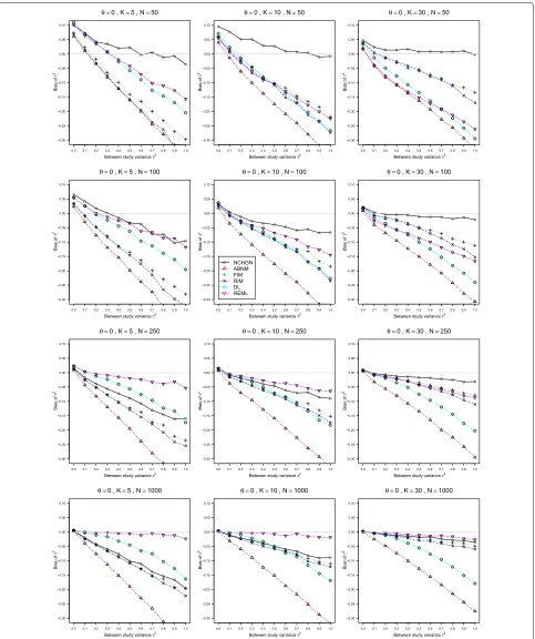
For all methods, the bias in the estimation of τ2
(Fig. 1 and Figure A4, Figure A7, Figure A8, Figure
A13, Figure A14 in the Additional file 2), is almost
lin-ear over the range of τ2, K and n. The bias is positive
for smaller values of τ2, where the GLMM with exact
noncentral hypergeometric-normal likelihood (NCHGN
method) provides the highest values whenn ≤ 100, but
otherwise is negative. The results for smaller sample sizes
(n≤ 100) differ from those for larger values ofn ≥250,
where the REML performs the best across the board, and always better than the DL [20] method. The bias of the
DL method is especially pronounced whenK ≥ 10. For
smaller sample sizes, the two main contenders for the
best estimation ofτ2are the exact NCHGN method and
the REML. The REML is always the best choice when
K = 5 but for the case of pi2 = 0.1, θ = 0,n = 50,
where the NCHGN is better for largeτ2. Similarly, when
K = 10, the NCHGN method is better than the REML
for larger τ2 and smaller n values when both
probabil-ities are small. The NCHGN method is always a good
choice when K = 30, and is the best for sparse data.
However, the REML is better for larger probabilities, see
Additional file 2: Figure A13 and Figure A14, and the
NCHGN behaves erratically for large sample sizes, as
can be seen in Fig. 4and is discussed in more detail in
“Computational issues” section. Bias of all the other
methods generally decreases with larger n and with
largerK, but for the GLMM with approximate
binomial-normal likelihood (ABNM), which performs the worst and appears to be asymptotically biased.
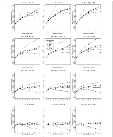
In respect to the estimation of the overall LORθˆ, all
methods perform well for larger probabilities (from 0.4)
in at least one arm, Additional file2: Figure A10 - Figure
A16, although the NCHGN behaves erratically forn =
1000, Additional file2: Figure A16. The distinctions are
clear only for relatively small probabilities in both arms, Fig. 2, Additional file 2: Figure A5 and Figure A9. The
estimates of the overall LOR θˆ are mostly considerably
positively biased. The only exceptions are the DL and
the REML based inverse variance methods for smallτ2,
and the conditional GLMM with approximate binomial-normal likelihood (ABNM) which often has large negative
bias. Overall, the ABNM has the lowest values ofθˆ, which
is an unexpected advantage for sample sizes up to 250
when pi2 ≤ 0.2, where the conditional GLMM with
exact likelihood, NCHGN, provides the second lowest
but still positively biased, values ofθˆ. The GLMM model
with random intercept, RIM, has the largest positive bias.
Bias increases with larger τ2, and may be considerable
for large values of τ2 and moderatenwhen pi2 ≤ 0.2.
For relatively sparse data and large values of τ2, the
NCHGN performs somewhat better than the standard methods DL and REML, which are very similar to each
other. Overall, the biases of the LORθˆare smaller when
piC > 0.1 in comparison to the case of sparse data in
both arms.
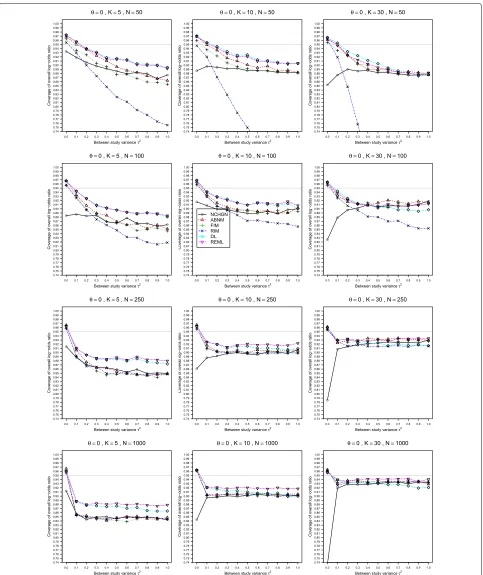
The coverage ofθ, Fig. 3 and Figure A6, Figure A11,
Figure A12, Figure A17, Figure A18 in the Additional file2, is closely related to the bias of its estimation. The coverage is typically lower than nominal, always for the
NCHGN, and for all but the smallest values ofτ2, below
0.1 or even lower whennis large, for all the other
meth-ods. The RIM has exceptionally low coverage for sparse
data. The coverage is strikingly better whenθ =1, where
it is above 90% for all methods except the NCHGN, but
it is unacceptably low whenθ = 0 where it deteriorates
Fig. 1Bias ofτ2in the REM whenp
i2=0.1,θ=0, 0≤τ2≤1 andn=50, 100, 250, 1000. Estimation methods are: pluses - unconditional
Fig. 2Bias ofθin the REM whenpi2=0.1,θ=0, 0≤τ2≤1 andn=50, 100, 250, 1000. Estimation methods are: pluses - unconditional
Fig. 3Estimated coverage ofθin the REM whenpi2=0.1,θ=0, 0≤τ2≤1 andn=50, 100, 250, 1000. The coverages are given at the nominal
95% level. Estimation methods are: pluses unconditional generalized linear mixedeffects model with fixed study effects (FIM), crosses
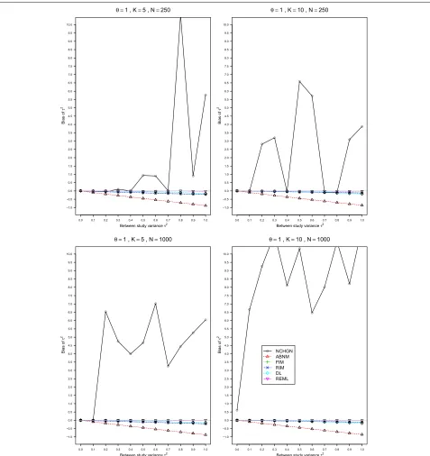
Fig. 4Bias ofτ2in the REM whenpi2=0.4,θ=1, 0≤τ2≤1 andn=50, 100, 250, 1000. Estimation methods are: pluses - unconditional
generalized linear mixed-effects model with fixed study effects (FIM), crosses - unconditional generalized linear mixed-effects model with random study effects (RIM), circles - a conditional generalized linear mixed-effects model with exact likelihood (NCHGN), triangles - a conditional generalized linear mixed-effects model with approximate likelihood (ABNM), rhombs - DerSimonian and Laird method (DL) and reverse triangles - restricted maximum likelihood method (REML). Light grey line at 0.95
NCHGN demonstrated the worst coverage at low values
of τ2, and a relatively stable, but still too low, coverage
under large heterogeneity. The coverage is very low, even
for large sample sizes, when the number of trialsK = 5
and improves for larger values of K, where increase in
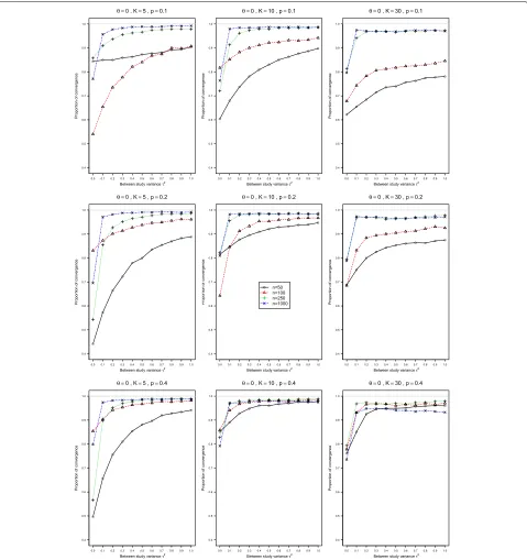
Fig. 5Proportion of convergence in the conditional generalized linear mixed-effects model with exact likelihood. These proportions of convergence are forpi2=0.1,pi2=0.2,pi2=0.4,θ=0, and 0≤τ2≤1 for sample sizesn=50, 100, 250, 1000 in each arm
Computational issues
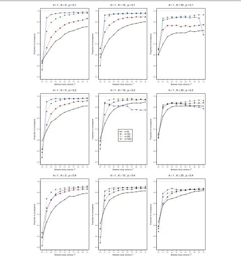
The convergence rates of the conditional GLMM with exact noncentral hypergeometric-normal likelihood (NCHGN) and the random intercept GLMM (RIM) methods implemented in the procedure rma.glmm in metaforwere rather low, see Figs.5and6for the NCHGN,
and Figure A19 and Figure A20 in the Additional file 5
for the RIM method. For the NCHGN method, the
convergence is the lowest atτ2 = 0, where it can be as
low as 40%, whereas for the RIM it is the lowest atτ2=1.
For both methods, the convergence is the worst for small probabilities, and improves for large sample sizes.
Fig. 6Proportion of convergence in the conditional generalized linear mixed-effects model with exact likelihood. These proportions of convergence are forpi2=0.1,pi2=0.2,pi2=0.4,θ=1, and 0≤τ2≤1 for sample sizesn=50, 100, 250, 1000 in each arm
sizes when the default “optim” optimizer is used. Some datasets result in anomalously large estimated values
of τ2 and, consequently, θ. This behavior is illustrated
by Fig. 4 (this is a blow-out of Figure A14 in the
Additional file2).
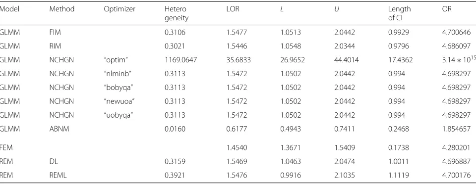
We provide an example of a simulated dataset causing
this problematic behaviour in Table2. The results of the
NCHGN with all the available optimizers in rma.glmm and also of the standard REM methods are provided in
Table3 and R code is given in Additional file6. All the
GLMMs except the ABNM and NCHGN with “optim”
result in very similar estimates of τˆ2 = 0.31, and the
LOR θˆ ≈ 1.55. The standard REM methods provide
Table 2Simulated data from REM withpiC=0.4,θ=1, τ2=0.6,K=5 andn1i=n2i=1000
y1i n1i−y1i n1i p1i y2i n2i−y2i n2i p2i θ OR
1 726 274 1000 0.726 401 599 1000 0.401 1.376 3.958
2 741 259 1000 0.741 406 594 1000 0.406 1.432 4.186
3 892 108 1000 0.892 378 622 1000 0.378 2.609 13.591
4 630 370 1000 0.63 415 585 1000 0.415 0.876 2.400
5 745 255 1000 0.745 404 596 1000 0.404 1.461 4.310
results inτˆ2 = 1169.06 and θˆ = 35.68. Such high
val-ues of biases even for one observation would considerably
increase the mean biases as can be seen in Fig.4. The
rea-son for this has to do with a bug in “optim” as the other optimizers provide consistent results. We also tried to reduce sample sizes in this simulated data by considering
datasets with all the values of yji and nji reduced by a
factor of a (and taking an integer part if needed), for
a=1.1, 1.2, 2, 3, 4, 5, 6, 9, 10. For all these smaller datasets, the NCHGN method with the “optim” optimizer either
has not converged (fora = 2, 6, 8 and 10), or resulted
in consistent estimates. We also tested other available in rma.glmm optimizers on these smaller datasets. They all converge every time, although the optimizer
“uobyqa” provides very different estimates of τ2 and θ
whena=6.
To check whether the results of our simulations are affected by the use of the default optimizer “optim”, we performed additional simulations (1000 repetitions per
configuration) for the problematic combination ofpi2 =
0.4, θ = 1, and also forpi2 = 0.1, θ = 1 forK = 5 and
10 andτ2∈[ 0, 1] using all the other available optimizers.
However, we discovered that the optimizer “uobyqa” just hangs when the other optimizers report non-convergence,
and we did not obtain further results from it. See the
Additional file7for an example.
For the first combination of parameters,pi2=0.4, θ =1,
the results on the convergence are summarised in
Addi-tional file 5: Figure A21, and for pi2 = 0.1, θ = 1 in
Additional file5: Figure A25. Results on the convergence
are similar for both configurations. The convergence is
always the worst atτ2=0 and slowly improves for higher
τ2 and for larger sample sizes. The convergence rates of
the “nlminb” are similar to that of the “optim”, about 40% at zero, but the “bobyqa” and “newbyqa” converge con-siderably more often, with 60 to 70% rates at zero. We
report the results on the bias ofτ2, and the bias and
cover-age ofθfor these two configurations when the alternative
optimizers are used in the next Section.
Simulation results for alternative optimizers
This Section summarises the results for the alternative
optimizers whenK=5 andK=10. Forpi2=0.4, θ =1
the results on the bias of τ2 and θ, and on the
cover-age ofθ are summarised in Figure A22 - Figure A24 in
the Additional file 5. When the sample sizes are 50 or
100, the “optim” behaves similarly to all the other
opti-mizers in respect to the bias of the estimation ofτ2, but
only this optimizer is unstable for larger sample sizes. For
all the other optimizers, the bias of the estimation ofτ2
is very similar, and does not much depend on the
sam-ple size n. The same is mostly true for the estimation
of θ, although the “nlminb” is not stable atτ2 = 0 for
n=1000.
However, the results of the coverage of θ, Additional
file 5: Figure A24, are strikingly different from those
obtained when using the “optim” (Additional file 2:
Figure A18). The coverage is approximately 85% with
the “optim”, but is considerably lower, especially for τ2
Table 3Meta-analysis of simulated data
Model Method Optimizer Hetero LOR L U Length OR
geneity of CI
GLMM FIM 0.3106 1.5477 1.0513 2.0442 0.9929 4.700646
GLMM RIM 0.3021 1.5446 1.0548 2.0344 0.9796 4.686097
GLMM NCHGN “optim” 1169.0647 35.6833 26.9652 44.4014 17.4362 3.14∗1015
GLMM NCHGN “nlminb” 0.3113 1.5472 1.0502 2.0442 0.994 4.698297
GLMM NCHGN “bobyqa” 0.3113 1.5472 1.0502 2.0442 0.994 4.698297
GLMM NCHGN “newuoa” 0.3113 1.5472 1.0502 2.0442 0.994 4.698297
GLMM NCHGN “uobyqa” 0.3113 1.5472 1.0502 2.0442 0.994 4.698297
GLMM ABNM 0.0160 0.6177 0.4943 0.7411 0.2468 1.854657
FEM 1.4540 1.3671 1.5409 0.1738 4.280201
REM DL 0.3159 1.5469 1.0463 2.0474 1.0011 4.696887
REM REML 0.3921 1.5476 0.9916 2.1035 1.1119 4.700176
near zero, for all the other optimizers. Examining the individual simulated datasets, we discovered that often, even when the NCHGN converges, the output includes
reasonable estimates ofτ2 andθ, but anomalously
pro-vides low values of the standard error ofθ, and therefore
extremely narrow confidence intervals. This finding is also discussed by [21].
The results for pi2 = 0.1, θ = 1 are provided in
Additional file 5: Figure A26 - Figure A28. The bias in
the estimation of τ2 is somewhat improved for large
sample sizes by the “newbyqa”, but both the “bobyqa” and
“nlminb” are worse at smalln and small τ2values. The
estimation ofθ using all the optimizers results in
some-what higher biases for smalln. Once more, the confidence
intervals for θ have very low coverage for small values
ofτ2.
We, therefore, believe that the results of the NCHGN
in respect to the bias of the estimation ofτ2 and θ for
n≤100 are not considerably affected by the choice of the
optimizer. The same is true for the results for larger sam-ple sizes whenever the “optim” behaves consistently. The
“optim” also appears to be the best optimizer whenτ2is
low. The coverage ofθ is the best with the “optim”.
Over-all, we agree with the choice of the “optim” as the default optimizer.
Example: effects of diuretics on pre-eclampsia
Data from nine trials that reported the effect of diuret-ics on pre-eclampsia [36] were studied by Hardy and Thompson [37], Biggerstaff and Tweedie [38], Turner et al. [16], Viechtbauer [35], Kulinskaya and Olkin [39], and Bakbergenuly and Kulinskaya [10].
The data are shown in Table 4 and were re-analysed
here in order to compare the results from the four GLMM models and additionally, the standard fixed effect and ran-dom effects models with inverse-variance weights. Except for the studies 3, 4 and 9, the incidence of pre-eclampsia in
both arms is below 0.15. The results are shown in Table5.
Table 4Data for meta-analysis on effects of diuretics on pre-eclampsia, [36]
study yi1 yi2 ni1 ni2 pi1 pi2
1 14 14 131 136 0.1068 0.1029
2 21 17 385 134 0.0545 0.1268
3 14 24 57 48 0.2456 0.5000
4 6 18 38 40 0.1579 0.4500
5 12 35 1011 760 0.0118 0.0460
6 138 175 1370 1336 0.1007 0.1310
7 15 20 506 524 0.0296 0.0382
8 6 2 108 103 0.0555 0.0194
9 65 40 153 102 0.4248 0.3921
The first two models are the GLMMs with fixed and ran-dom study effects given by (2) and (5), respectively. The second two models are the conditional GLMMs with exact and approximate likelihood given by (8) and (9). Both the DL [20] and REML estimation results are provided for the REM.
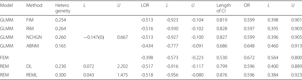
The first three GLMMs give very similar estimates of
the between-study variance τ2, varying from 0.254 to
0.264. The GLMM with approximate likelihood (ABNM) resulted in a noticeably lower value, 0.165. The standard REM results in 0.230 for the DerSimonian-Laird (DL), and
0.300 for the REML estimate ofτ2, respectively. The use of
the REML in the REM was recommended by Viechtbauer [40] as the least biased and the most efficient estimate of
τ2. However, Turner et al. [16] analysed the current
exam-ple and showed thatτˆREML2 is biased downward. We agree
with their view and believe that all these estimates ofτ2
are too low, on the basis of the results of our simulations. For the estimation of the LOR, the first three GLMMs
give very similar estimates,−0.513 and−0.516, and these
estimates are very close to those from the REM,−0.517
and −0.518. Once more, the estimate from the
condi-tional GLMM with approximate likelihood is very
dif-ferent,−0.434. However, this estimate may well be very
close to the true value. In our simulations, this model pro-vided a consistently lower estimate of the LOR than the three other GLMMs, and for the similar sample sizes (an average arm size 386) and heterogeneity of approximately 0.25 in this example, the ABNM was almost unbiased in the estimation of the LOR. The widths of the confi-dence intervals for the LOR correspond to the estimated
τ2values; the REM with the REML has the widest
confi-dence interval, followed by the GLMM with random study effects (RIM) and the conditional GLMM with exact like-lihood (NCHGN). The approximate ABNM model gives the narrowest confidence interval, however, our simula-tions suggest that it may well have the best coverage when
θ =0 and the worst coverage whenθ =0.
Discussion
We examined by simulation the performance of gener-alized linear mixed models with exact and approximate likelihood, when applied to the meta-analysis of log odds ratios. The models were applied to data simulated from a binomial-normal model; that is, from a pair of binomial distributions within each study, with the logarithm of odds ratio normally distributed across studies.
When the sample sizes are small and binary out-comes are sparse, it is well known that the standard methods of meta-analysis have considerable bias in the
estimation of both τ2 and θ. This is also
Table 5Meta-analysis of diuretics in pre-eclampsia
Model Method Hetero L U LOR L U Length OR L U
geneity of CI
GLMM FIM 0.254 -0.513 -0.923 -0.104 0.819 0.599 0.398 0.901
GLMM RIM 0.264 -0.516 -0.930 -0.102 0.828 0.597 0.395 0.903
GLMM NCHGN 0.260 −0.147(0) 0.667 -0.513 -0.927 -0.100 0.827 0.599 0.396 0.905
GLMM ABNM 0.165 -0.434 -0.777 -0.091 0.686 0.648 0.460 0.913
FEM -0.398 -0.573 -0.223 0.530 0.672 0.564 0.800
REM DL 0.230 0.072 2.202 -0.517 -0.916 -0.117 0.799 0.596 0.400 0.889
REM REML 0.300 0.043 1.475 -0.518 -0.956 -0.080 0.876 0.596 0.384 0.923
Estimates and confidence intervals (CIs) for the heterogeneity parameterτ2, for the overall log-odds-ratio (LOR) and for the overall odds ratios (OR); GLMM is the generalized
linear mixed model, REM is the random-effects model and FEM is the fixed-effect model.LandUare the lower and upper limits of the respective 95% confidence intervals
generalized linear mixed model with an exact noncen-tral hypergeometric-normal likelihood was suggested as an alternative to the standard random effects model. Our simulations showed that the standard REML-based
esti-mation works well for large studies (from n = 250)
and/or large event probabilities, but the NCHGN method provides considerably less biased estimation of the
hetero-geneity varianceτ2than all the other methods, including
the DL and the REML methods, when the data are sparse, the sample sizes are small, and especially so for the large number of studies or for moderate to large values of
τ2. However, our simulations demonstrated that the
esti-mates of the LORθare considerably positively biased for
all the studied methods, including the conditional GLMM with an exact noncentral hypergeometric likelihood, when
θ = 0. These biases, combined with the underestimation
of the standard error of θ by the NCHGN and ABNM,
resulted in coverage lower than the nominal confidence
level of 0.95 forθ. We did not study the coverage of wider
confidence intervals based on t critical values, as these
intervals would still provide lower than nominal cover-age due to aforementioned biases. One of the limitation of the conditional GLMM with approximate likelihood is that the assumption of small total numbers of events rel-ative to the total group sizes is too strong and rare in real data meta-analysis of binary outcomes. In our simu-lations, this method performed considerably worse than
the exact method for the estimation of τ2, and we do
not recommend it. The two other models, with the fixed and the random study effects, were somewhere between the two conditional methods, although the random
inter-cept model resulted in the largest positive bias forθ, and
therefore cannot be recommended. The REML method performed the best in respect to the coverage of the log
odds ratioθ.
The R package metafor can use either of two
meth-ods for fitting the conditional generalized linear mixed model with exact likelihood. The default method uses
the density function dFNCHypergeo from the
Biase-dUrn package. The second method uses the density
function dnoncenhypergeom from theMCMCpack
pack-age. The stability and performance of the two meth-ods are similar. There are computational issues to do with the default optimizer “optim” used in the NCHGN method when the sample sizes are large,
espe-cially when the between-studies variance τ2 is
consid-erable. However, the other optimizers are also dogged by computational issues, and overall perform worse.It would be certainly of interest to repeat our simulations using SAS.
Conclusions
To summarise, even though there is no uniformly best method for estimating the between-study variance and overall effect measure, we recommend using the REML
for the point and interval estimation of θ, whereas the
NCHGN may be used for the estimation ofτ2when the
sample sizes are small and the data are sparse. When the sample sizes are large, we recommend using the REML
instead of the NCHGN for the estimation ofτ2. Finally, no
methods perform well when the number of studies is very
small (K=3), especially for sparse data, but the REML is
somewhat better overall.
The design of our simulations, which used equal sample sizes and equal probabilities in all studies may be consid-ered a limitation. However, we would not expect better performance of the GLMMs in a more realistic scenario. At the moment, it is difficult to recommend the use of GLMMs in the practice of meta-analysis.
We believe that the bias in the estimation of θ in
biases of order 1/N are well known in fixed effect and mixed effects models. Nemes et al. [41] show that logis-tic regression overestimates the odds ratio because of
bias of order 1/N in studies with small and moderate
sample sizes. Kosmidis et al. [42] studied bias of order
1/N in the maximum-likelihood estimates of the
over-all effect measure and the between-study variance under the normal random-effects model. However, the transfor-mation biases in the mixed effects models are of order 1, as discussed in [6]. The problem of finding reasonably good methods of the meta-analysis for binary outcomes is still open.
Additional files
Additional file 1:- metafor syntax for GLMM in R. This file provides
information on implementation of GLMM models in R metafor package. (PDF 77 kb)
Additional file 2:- Simulation results forpi2=0.1,pi2=0.2 andpi2=0.4
under default settings. This file provides additional simulation results under default settings of rma.glmm function in R metafor package. (PDF 586 kb)
Additional file 3:- Simulation results for K=3,pi2=0.1,θ=0 andθ=1
under default settings. (PDF 223 kb)
Additional file 4:- Simulation results for comparison of dFNCHypergeo
and dnoncenhypergeom in a conditional GLMM with exact likelihood. This file provides results of simulations with two methods for fitting the non-central hypergeometric distribution in R (PDF 147 kb)
Additional file 5:- Computational issues. This file provides Figures for
convergence and estimation quality of alternative optimizers. (PDF 232 kb)
Additional file 6:- R code for GLMM analysis of simulated data in
“Computational issues” section. This file provides R code for GLMM analysis of simulated data in “Computational issues” section. (PDF 122 kb)
Additional file 7:- R code for an example where the optimizer “uobyqa”
hangs. This file provides R code and output for an example where the optimizer “uobyqa” hangs. (PDF 107 kb)
Abbreviations
ABNM: binomial-normal model; CM.AL: Inmetafor, a conditional generalized linear mixed-effects model (approximate likelihood); CM.EL: Inmetafor, a conditional generalized linear mixed-effects model (exact likelihood); DL: Der-Simonian and Laird ;REML: restricted maximum likelihood; EM: Expectation maximization; FEM: Fixed effect model; FIM: Fixed intercept model; GEE: Generalized estimation equation, GHQ: Gauss-Hermite quadrature; GLMM: Generalized linear mixed models; LOR: Log-odds ratio; MCMC: Markov-chain Monte Carlo; NCHGN: Non-central-hypergeometric-normal model; OR: Odds ratio; PQL: Penalized quasi likelihood; REM: Random effects model; RIM: Random intercept model; RR: Relative risk; UM.FS: Inmetafor, an unconditional generalized linear mixed-effects model with fixed study effects; UM.RS: In
metafor, an unconditional generalized linear mixed-effects model with random study effects
Acknowledgements
The authors thank Wolfgang Viechtbauer for preliminary discussions of simulation results, David C. Hoaglin for many useful comments on an early draft of this article, and Daniel Jackson and Ian White for useful discussion of models and comparison of simulation results. The authors also thank the referees, Han Du and Oliver Kuss, and the associate editor Fang Liu for their useful suggestions for improving the presentation of the material of this article.
Funding
The work by E. Kulinskaya was supported by the Economic and Social Research Council [grant number ES/L011859/1].
Availability of data and materials
All simulation results are depicted in Figures in the main text and in the Additional Files, and are available from authors on reasonable request. The data for an example in “Example: effects of diuretics on pre-eclampsia” section is given in Table4.
Authors’ contributions
Both authors have made contributions to conception, design and methodology of this study. IB carried out the simulations, and EK drafted the first version of the manuscript. Both authors have been involved in revisions, read and approved the final manuscript.
Ethics approval and consent to participate
Not applicable.
Consent for publication
Not applicable.
Competing interests
The authors declare that they have no competing interests.
Publisher’s Note
Springer Nature remains neutral with regard to jurisdictional claims in published maps and institutional affiliations.
Received: 22 February 2018 Accepted: 24 June 2018
References
1. Higgins J, Thompson SG, Spiegelhalter DJ. A re-evaluation of random-effects meta-analysis. J R Stat Soc Ser A (Stat Soc). 2009;172(1): 137–59.
2. Mosteller F, Colditz GA. Understanding research synthesis (meta-analysis). Annu Rev Public Health. 1996;17(1):1–23.
3. Stijnen T, Hamza TH, Özdemir P. Random effects meta-analysis of event outcome in the framework of the generalized linear mixed model with applications in sparse data. Stat Med. 2010;29(29):3046–67.
4. Kulinskaya E, Morgenthaler S, Staudte RG. Combining statistical evidence. Int Stat Rev. 2014;82(2):214–42.
5. Hoaglin DC. Misunderstandings aboutQand ’Cochran’sQtest’ in meta-analysis. Stat Med. 2016;35(4):485–95.https://doi.org/10.1002/sim. 6632. sim.6632.
6. Bakbergenuly I, Kulinskaya E, Morgenthaler S. Inference for binomial probability based on dependent Bernoulli random variables with applications to meta-analysis and group level studies. Biom J. 2016;58(4): 896–914.
7. Viechtbauer W. Packagemetafor. The Comprehensive R Archive Network. Package ‘metafor’.http://cran.r-project.org/web/packages/metafor/ metafor.pdf. 2017. Accessed 19 Feb 2017.
8. Lee KJ, Thompson SG. Flexible parametric models for random-effects distributions. Stat Med. 2008;27:418–34.
9. Kuss O. Statistical methods for meta-analyses including information from studies without any events—add nothing to nothing and succeed nevertheless. Stat Med. 2015;34(7):1097–116.
10. Bakbergenuly I, Kulinskaya E. Beta-binomial model for meta-analysis of odds ratios. Stat Med. 2017;36(11):1715–34.
11. Sinclair JC, Bracken MB. Clinically useful measures of effect in binary analyses of randomized trials. J Clin Epidemiol. 2014;47:881–9. 12. Sackett DL, Deeks JJ, Altman DG. Down with odds ratios!. Evid-Based
Med. 1996;1:164–6.
13. Altman DG, Deeks JJ, Sackett DL. Odds ratios should be avoided when events are common (letter to the editor). BMJ. 1998;317:1318.
14. Deeks JJ. Issues in the selection of a summary statistic for meta-analysis of clinical trials with binary outcomes. Stat Med. 2002;21:1575–600. 15. Newcombe RG. A deficiency of the odds ratio as a measure of effect size.
Stat Med. 2006;25:4235–40.
16. Turner RM, Omar RZ, Yang M, Goldstein H, Thompson SG. A multilevel model framework for meta-analysis of clinical trials with binary outcomes. Stat Med. 2000;19(24):3417–32.
18. Liu Q, Pierce DA. Heterogeneity in Mantel-Haenszel-type models. Biometrika. 1993;80(3):543–56.
19. Sidik K, Jonkman JN. Estimation using non-central hypergeometric distributions in combining 2×2 tables. J Stat Plan Infer. 2008;138(12): 3993–4005.
20. DerSimonian R, Laird N. Meta-analysis in clinical trials. Control Clin Trials. 1986;7(3):177–88.
21. Jackson D, Law M, Stijnen T, Viechtbauer W, White IR. A comparison of 7 random-effects models for meta-analyses that estimate the summary odds ratio. Stat Med. 2018;37(7):1059–85.
22. Breslow NE, Clayton DG. Approximate inference in generalized linear mixed models. J Am Stat Assoc. 1993;88(421):9–25.
23. Demidenko E. Mixed Models: Theory and Applications. Hoboken: Wiley; 2004.
24. Capanu M, Gönen M, Begg CB. An assessment of estimation methods for generalized linear mixed models with binary outcomes. Stat Med. 2013;32(26):4550–66.https://doi.org/10.1002/sim.5866.
25. Platt RW, Leroux BG, Breslow N. Generalized linear mixed models for meta-analysis. Stat Med. 1999;18(6):643–54.
26. Gao S. Combining binomial data using the logistic normal model. J Stat Comput Simul. 2004;74(4):293–306.
27. Hamza TH, Van Houwelingen HC, Stijnen T. The binomial distribution of meta-analysis was preferred to model within-study variability. J Clin Epidemiol. 2008;61(1):41–51.
28. Liang KY, Zeger SL. Longitudinal data analysis using generalized linear models. Biometrika. 1986;73(1):13–22.
29. Viechtbauer W. Conducting meta-analyses inRwith themetaforpackage. J Stat Softw. 2010;36(3):1–48.
30. Liang KY. Odds ratio inference with dependent data. Biometrika. 1985;72(3):678–82.
31. Fog A, Fog MA. TheBiasedUrnpackage inR. 2015.http://cran.r-project. org/web/packages/BiasedUrn/BiasedUrn.pdf. Accessed 19 Feb 2017. 32. Martin AD, Quinn KM, Park JH, Park MJH. TheMCMCpackpackage inR.
2016.https://cran.r-project.org/web/packages/MCMCpack/MCMCpack. pdf. Accessed 19 Feb 2017.
33. Gay DM. Usage summary for selected optimization routines. Comput Sci Tech Rep. 1990;153:1–21.
34. Powell MJ. The bobyqa algorithm for bound constrained optimization without derivatives. Cambridge: Cambridge NA Report NA2009/06, University of Cambridge; 2009. pp. 26–46.
35. Viechtbauer W. Confidence intervals for the amount of heterogeneity in meta-analysis. Stat Med. 2007;26(1):37–52.
36. Collins R, Yusuf S, Peto R. Overview of randomised trials of diuretics in pregnancy. Br Med J (Clin Res Ed). 1985;290(6461):17–23.
37. Hardy RJ, Thompson SG. A likelihood approach to meta-analysis with random effects. Stat Med. 1996;15(6):619–29.
38. Biggerstaff BJ, Tweedie RL. Incorporating variability in estimates of heterogeneity in the random effects model in meta-analysis. Stat Med. 1997;16(7):753–68.
39. Kulinskaya E, Olkin I. An overdispersion model in meta-analysis. Stat Model. 2014;14(1):49–76.
40. Viechtbauer W. Bias and efficiency of meta-analytic variance estimators in the random-effects model. J Educ Behav Stat. 2005;30(3):261–93. 41. Nemes S, Jonasson J, Genell A, Steineck G. Bias in odds ratios by logistic
regression modelling and sample size. BMC Med Res Methodol. 2009;9(1):1. 42. Kosmidis I, Guolo A, Varin C. Improving the accuracy of likelihood-based
![Table 4 Data for meta-analysis on effects of diuretics onpre-eclampsia, [36]](https://thumb-us.123doks.com/thumbv2/123dok_us/9216343.1916752/15.595.56.291.592.733/table-data-meta-analysis-effects-diuretics-onpre-eclampsia.webp)