Identical and Nonidentical Synchronization of Hyperchaotic Systems by Active Backstepping Method

Identical and Nonidentical Synchronization of Hyperchaotic

Systems by Active Backstepping Method

A. Abooee* and M. R. Jahed-Motlagh*

Abstract: This paper deals with the tracking and synchronization problems of hyperchaotic systems based on active backstepping method. The mentioned method consists of a recursive approach that interlaces the choice of a Lyapunov function with the design of feedback control. At first, a nonlinear recursive active backstepping control vector is designed such that state variables of the hyperchaotic Wang system track desired trajectories. Furthermore, this method is applied to synchronize two identical hyperchaotic Wang systems. Eventually, it is used to implement synchronization between hyperchaotic Wang system and hyperchaotic Rössler system. Numerical simulations are performed to demonstrate the effectiveness and efficiency of the three designed active backstepping control vectors.

Keywords: Hyperchaotic System, Identical Synchronization, Backstepping Methods,

Rössler and Wang Systems.

1 Introduction1

In general, a hyperchaotic system is defined as a chaotic system with at least two positive exponents, implying that its dynamics are extended in several different directions simultaneously [1]. The first hyperchaotic system was introduced by Rössler [2] which represents dynamical equations of a particular chemical reaction. Recently, many new hyperchaotic systems were introduced by scientists of various fields [3-7] and synchronization problem of the hyperchaotic systems has become a hot topic among researchers [8-14] due to wide applications of synchronization of hyperchaotic systems in many engineering field such as secure communications [15-17], image encryption [18, 19], lasers [20, 21].

In recent decades, different methods have been proposed to synchronize hyperchaotic systems including adaptive control [22], fuzzy control [23], active control [14] sliding mode control [24], impulsive control [8], backstepping method [25-30] and so on.

In particular, backstepping recursive nonlinear control scheme has been widely employed to synchronize and control of hyperchaotic systems which can be continuous-time [25, 26] or discrete-time [27]. It is well known that backstepping method represents a

Iranian Journal of Electrical & Electronic Engineering, 2012. Paper first received 9 Nov. 2011 and in revised form 10 May 2012. * The Authors are with the Complex Systems Lab, Department of Computer Engineering,Iran University of Science and Technology, Tehran, Iran.

E-mails: [email protected], [email protected].

powerful and systematic technique that recursively interlaces the choice of a Lyapunov function with the design of feedback control. The mentioned method can guarantee global stability, tracking and transient performance for a broad class of strict-feedback nonlinear systems and control goal can be achieved with reduced control effort. Motivated above discussion, in this paper three novel active control vectors based on the backstepping method are proposed to control and synchronize the Wang and Rössler hyperchaotic systems. The advantages of proposed method can be summarized as follows: (a) it is a systematic procedure for hyperchaos control and synchronization of hyperchaotic systems and guarantees the stability of the closed-loop system; (b) The proposed method can overcome the controller singularity problem resulting from the nonlinear term of quadratic type; (c) it can be applied to a variety of hyperchaotic systems no matter whether it contains external excitation or not; (d) there is no derivatives in controllers, so it is easy to be implemented.

The rest of this paper is organized as follows. Section 2 presents two dynamic models of the hyperchaotic Wang and Rössler systems. In Section 3, the tracking problem for hyperchaotic Wang system is investigated by using backstepping method. In Section 4, an active backstepping control vector is designed to synchronize two identical hyperchaotic Wang systems. In Section 5, the generalized synchronization between the hyperchaotic Rössler system and the hyperchaotic Wang system is achieved by using the backstepping

controllers. Numerical simulation results which that confirm the validity and feasibility of the designed controllers are shown in Section 6. Finally, conclusions are given in Section 7.

2 Descriptions of Wang and Rössler Systems

In order to synchronize hyperchaotic Wang and Rössler systems, a brief review of their models is expressed in this section. In 1979, Rössler [2] introduced a four-dimensional hyperchaotic system containing only one nonlinear quadratic term. Due to its simplicity, the Rössler system has become a standard benchmark hyperchaotic system to verify different control methods of hyperchaos phenomenon. Numerical

calculations show that the mentioned system has two

positive Lyapunov exponents, namely, L1=0.11 and

1 0.02

L = . In fact, the Rössler system describes a

chemical reaction scheme [2]. The differential equations of Rössler system are given by

1 2 1

2 2 3

3 2 4

4 1 3 4

3

y y y

y y y

y y y

y y y y

= +

= +

= − −

= + +

& & & &

β

γ

α

(1)

where y i_i, =1,_K, 4 are the state variables of Rössler

system, and α, β γ, are constant parameters. When

parameters are considered asα=0.25, β = −0.5 and

= 0.05

γ , system (1) shows hyperchaotic behaviors.

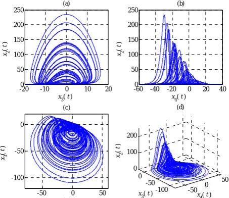
Figs. 1(a), (b), (c) depict the projections of hyperchaotic attractor of the system (1) onto x2−x3,x2−x4, x3−x4

planes, respectively. Fig. 1(d) displays the trajectory of the system (1) plotted in x2−x3−x4 space.

-200 -10 0 10 20 50

100 150 200 250

x( 2 t )

x

3( t )

(a)

-600 -40 -20 0 20 40 50

100 150 200 250

x( 2 t )

x

4( t )

(b)

-50 0 50 -100

-50 0

x3

(

t

)

x₄( t ) (c)

-50 0 50 -100

-50 0 0 100 200

x₄( t ) (d)

x

3( t )

x( 2 t )

Fig. 1 Projections of hyperchaotic attractor of the Rössler

system: (a) Projection onto x₂−x₃ plane, (b) Projection onto

2 4

x −x plane, (c) Projection of onto x3−x4 plane, (d)

Three-dimensional view in x2−x3−x4 space.

Wang [31] proposed a new hyperchaotic system by introducing an additional state into the third-order Liu chaotic system [32]. The four-dimensional autonomous hyperchaotic system is described by

2

1 1 2

2 3 2

3 2 1 2 4

4 2

( )

x cx hx

x a x x

x bx kx x x

x dx

= − +

= −

= − +

= −

& & & &

(2)

where x i_i, =1,_K, 4 are the state variables of Rössler

system, and a b c d h k, , , , , are positive constant

parameters. When parameters are a=10, b=40,

2.5

c= , d=10.6, k=1 and h=4, system (2) is

hyperchaotic with two positive Lyapunov exponent

1 1.15

L = , L2=0.13. The system (2) has only one

equilibrium point at the origin, and the equilibrium point is an unstable saddle node considering mentioned parameters [33]. Figs. 2(a), (b), (c) show the projections of hyperchaotic attractor of Wang system onto x1−x2,

2 3

x −x and x3−x4 planes respectively. Fig. 2(d)

depicts the trajectory of Wang system plotted in

2 3 4

x −x −x space.

3 Tracking Problem for Wang System

In this section, backstepping method is used to design active controllers to suppress hyperchaos in the hyperchaotic Wang system. The controlled hyperchaotic Wang system [31] is given by

0 50 100 -20

-10 0 10 20

x2

(

t

)

x₁( t ) (a)

-20 -10 0 10 20 -40

-20 0 20

x( 3 t )

x₂( t ) (b)

-40 -20 0 20 -50

0 50

x4

(

t

)

x

3( t )

(c)

0 50 100 -20

0 20 -40 -20 0 20

x

1( t )

(d)

x

2( t )

x3

(

t

)

Fig. 2 Projections of hyperchaotic attractor of the system (2):

(a) Projection onto x1−x2 plane, (b) Projection onto x2−x3

plane, (c) Projection onto x3−x4 plane, (d)

Three-dimensional view of hyperchaotic attractor.

2 1 1 2 1 2 3 2 2 3 2 1 2 4 3 4 2 4

( )

x cx hx u

x a x x u

x bx kx x x u

x dx u

= − + +

= − +

= − + +

= − +

& & & &

(3)

Our main goal is to design an appropriate active

backstepping control vector = [ ,1 2, 3, 4]

T

u u u u

u such

that the controlled system (3) can track desired trajectory x t_d( ) with a scalar output x t1( ) in the sense that

1

lim d 0

t→∞ x −x = (4)

The backstepping design procedure is recursive. At the _ith

step, the _ith

-order subsystem is stabilized with respect to a Lyapunov function by the design of a virtual

control ϕi and a control input ui.Now, we begin to

design the active controllers based on the backstepping design method as follows.

Step 1. Assume that η1= −x1 xd, then its derivative

is derived as

2

1= −x1 xd = −c( 1+xd)+hx2−xd+u1

& & & &

η η (5)

where x2 =ϕ η1( )1 is considered as a virtual controller. To design ϕ η1( )1 such that stabilizes η1-subsystem (5), the following Lyapunov function V1 is selected.

2 1 0.5 1

V =

η

(6)

Then, the derivative of V1 is concluded as

2

1 1 1 1( 1 1( )1 d d 1)

V& =η η η& = −cη +hϕ η −cx − +x_& u (7) Here, we choose ϕ η₁( )₁ =0 and u₁ =cx_d +x_&d such

that 2

1 1

V& = −cη is negative definite. This implies that the

1

η -subsystem (5) is stable. Since the virtual control

function ϕ η1( )1 is estimative, an error variable is

defined as follows

2=x2− 1( )1

η

ϕ η

(8)

The following (η η1− 2)-subsystem can be obtained as

2 1 1 2 2 3 2 2

c h

a x a u

= − +

= − +

& &

η

η

η

η

η

(9)

where x₃ =ϕ η η₂( ,_{1 2}) is regarded as a virtual controller. Step 2. In order to stabilize the (η η1− 2)-subsystem (9), the Lyapunov function V₂ is defined as follows.

2 2 1 0.5 2

V = +V η (10)

The derivative of V2 is yielded as

2 2 2

2 1 1 2 2 2( ,1 2) 2 2 2

V& = −c

η

+h

η η

+a

η ϕ η η

−a

η η

+ u (11)

If ϕ η η₂( ,_{1 2})=0 and u₂ = −hη η_{1 2}, then

2 2

2 1 2 0

V& = −cη −aη < concludes that the (η η1− 2)

-subsystem (9) is stable. Since the virtual control

function ϕ η η2( ,1 2) is estimative, an error variable is defined as follows.

3=x3− 2( ,1 2)

η

ϕ η η

(12)

Then the following (η η η₁− ₂− ₃)-subsystem is

obtained as

2 1 1 2 2 3 2 1 2

3 2 2 1 4 3

( )

( _d)

c h

a h

b k x x u

= − +

= − −

= − + + +

& & &

η η η

η η η η η

η η η η

(13)

where x4=ϕ η η η3( ,1 2, 3) is regarded as a virtual controllers.

Step 3. In order to stabilize the (η η η₁− ₂− ₃)

-subsystem (13), the Lyapunov function V3 is selected as follows.

2 3 1 2 0.5 3

V =V +V + η (14)

The derivative of V3 is given by

2 2

3 1 2 2 3 1 2 3 2 3 3 3 1 2 3 3 3

( )

( , , )

d

V c a a b k

k x u

= − − + + −

− + +

& η η η η η η η

η η η ϕ η η η η (15)

Then, we choose ϕ η η η3( ,1 2, 3) and

(

)

3 2 1 2 2 d 3

u = − +a b η +kη η +kη x −η such that

2 2 2

3 1 2 3 0

V&=−cη −aη η− < is negative definite. This implies

that the (η η η1− 2− 3)-subsystem (13) is stable.

Similarly, assume that η4=x4−ϕ η η η3

(

1, 2, 3

)

then the following subsystem is concluded.

2 1 1 2 2 3 2 1 2 3 2 4 3 4 2 4

( )

c h

a h

a

d u

= − +

= − −

= − + −

= − +

& & & &

η η η

η η η η η

η η η η

η η

(16)

Step 4. In order to stabilize the (η η η η1− 2− −3 4)

-system (16), a Lyapunov function V4 is considered as

follows.

2

4 1 2 3 0.5 4

V = +V V + +V η (17)

The derivative of V₄ is given by

2 2 2

4 1 2 3 3 4 2 4 4 4

V& = −cη −aη −η +η η −dη η η+ u (18)

If we choose u4 = − −η η4 3+dη2, then

2 2 2 2

4 1 2 3 4 0

V& = −cη −aη −η −η < , therefore

1 2 3 4

(η η η η− − − )-system (16) is stable. Since V&₄ is

negative definite, it follows that in the

1 2 3 4

(η η η η− − − )coordinates the equilibrium (0, 0, 0, 0)

is stable. By considering η1= −x1 x td( ), η2 =x2,

3 =x3

η and η4 =x4, one can clearly conclude that the

state variable x t1( ) of controlled Wang system (3),

tracks the desired trajectory x t_d( ).

4 Synchronization of Two Identical Wang Systems In this section, two identical hyperchaotic Wang systems are considered as master and slave systems respectively. The master system is described as Eq. (2), and the slave system is given by

2 1 1 2 1 2 3 2 2 3 2 1 2 4 3 4 2 4

( )

y cy hy u

y a y y u

y by ky y y u

y dy u

= − + +

= − +

= − + +

= − +

& & & &

(19)

where [ ,1 2, 3, 4]

T

x x x x =

x stands for the state variables

vector of the master system, [ ,1 2, 3, 4]

T

y y y y =

y denotes

the state variables vector of the slave system and

1 2 3 4

[ ,u u u u, , ]T =

u is the control inputs vector.

Our goal is to design an appropriate active backstepping control inputs vector u( )t ∈ 4 such that the state variables of the slave system track the ones of the master system in the sense that

lim 0

t→∞ y−x = (20)

where . is the Euclidean norm. By defining the

synchronization errors vector as

1 2 3 4

[ , , , ] ,T ,

i i i

e e e e e y x

= = −

e i = 1, 2, 3, 4, we can

subtract Eq. (19) from Eq. (2), which yields the following synchronization error system.

2

1 1 2 2 2 1 2 3 2 2

3 2 4 1 2 1 2 2 1 3 4 2 4

2

( )

( )

e ce h e h x e u

e a e e u

e be e k e e x e x e u

e d e u

= − + + +

= − +

= + − + + +

= − +

& & & &

(21)

Therefore, the identical synchronization problem is reduced to the stabilization problem of the

synchronization error system (21). Consequently, the

control inputs vector u( )t should be designed to

stabilize the system (21). Finally, the stabilization of the system (21) implies that the master and slave Wang systems are synchronized properly. Now, the active controllers will be designed based on the backstepping method as follows.

Step1. Let µ1=e1, then its derivative can be obtained a

2

1= −c 1+he2+2h x e2 2+u1

&

μ μ (22)

where e₂ =ϕ₁( )µ₁ can be regarded as a virtual

controller. To design of ϕ1(µ1) and u1 such that

stabilize µ₁-subsystem (22), the following Lyapunov

function V1 is considered as follows. 2

1 0.5 1

V = μ (23)

Then, the derivative of V₁ is obtained as 2

1 1[ 1( 1) 2 2 1( 1) 1 1]

V& =μ ϕ μh + h x ϕ μ −cμ +u (24)

If we choose ϕ1(µ1)=u1=0, then

2

1 1 0

V& = −cμ < is

negative definite. This implies that the µ1-subsystem

(22) is stable. Since the virtual control function ϕ1(µ1) is estimative, the error between e2and ϕ1(µ1)is defined as

2 =e2− 1( 1)

μ ϕ μ (25)

Then, the (μ μ₁− ₂)-subsystem can be derived as

2

1 1 2 2 2

2 3 2 2

2

c h hx

a e a u

= − + +

= − +

& &

μ μ μ μ

μ μ (26)

where e3=ϕ2( ,µ µ1 2) can be considered as a virtual controller.

Step 2. In order to stabilize the (μ μ1− 2)-subsystem (26), the Lyapunov function V2 is defined as

2 2 1 0.5 2

V = +V μ (27)

The derivative of V₂ is given by

2 2 2

2 1 2 2 1 2 1 2 2 2 1 2 2 2

2

( , )

V h hx c a

a u

= + − − +

+ +

& μ μ μ μ μ μ

μ ϕ μ μ μ (28)

If ϕ μ μ2( 1, 2)=0 and u2 = −hµ µ1 2−2hx µ2 1, then

2 2

2 1 2 0

V& = −cμ −aμ < , which implies the (μ μ1− 2) -subsystem (26) is stable. Similarly, assume that

3 3 2( ,1 2)

µ = −ϕe µ µ , then the following (μ μ1− 2−μ3)

-system can be derived.

2

1 1 2 2 2 2 3 2 1 2 2 1

3 2 4 1 2 1 2 2 1 3

2

2

( )

c h hx

a a h hx

b e k x x u

= − + +

= − − −

= + − + + +

& & &

μ μ μ μ

μ μ μ μ μ μ

μ μ μ μ μ μ

(29)

where e4 =ϕ3( ,µ µ µ1 2, 3) can be regarded as a virtual controller.

Step 3. The Lyapunov function V3 is defined by 2

3 2 1 0.5 3

V =V + +V μ (30)

In order to make (µ₁−µ₂−µ₃)subsystem (29)

stable, the derivative of V3 is given by

2 2

3 1 2 2 3 1 2 3 2 1 3 3 3 1 2 3 3 3

( )

( , , )

V c a a b kx

kx u

= − − + + −

− + +

& μ μ μ μ μ μ

μ μ μ ϕ μ μ μ μ (31)

We can choose ϕ3( ,µ µ µ1 2, 3)= −µ3 and

3 ( ) 2 1 2 1 2 2 1

u = − +a b µ +kµ µ +kx µ +kx µ , so that

2 2 2

3 1 2 3 0

V& = −cμ −aμ −μ < , which verifies the

1 2 3

(µ −µ −µ)-subsystem (29) is stable.

Let µ4=e4− ( ,ϕ3 µ µ µ1 2, 3), then the following

1 2 3 4

(µ −µ −µ −µ)-system is concluded.

2

1 1 2 2 2 2 3 2 1 2 2 1 3 2 4 3

4 2 4 3 4

2

2

( )

c h hx

a a h hx

a

d a u

= − + +

= − − −

= − + −

= − + + − +

& & & &

μ μ μ μ

μ μ μ μ μ μ

μ μ μ μ

μ μ μ μ

(32)

Step 4. In order to stabilize the (µ1−µ2−µ3−µ4)

-system (32), the Lyapunov function V4 defined by Eq.

(33).

2 4 1 2 3 0.5 4

V =V +V +V + μ (33)

The derivative of V₄ is expressed as

2 2 2 2 4 1 2 3 4 2 4 4 4

( )

V c a

d a u

= − − − +

− + +

& μ μ μ μ

μ μ μ (34)

If u4=(d+a µ) 2−2µ4, then

2 2 2 2

4 1 2 3 4 0

V& = −cμ −aμ −μ −μ < proves that the

1 2 3 4

(µ −µ −µ −µ)-system (32) is stable. Finally, the

1 2 3 4

(µ −µ −µ −µ)-system is described by

2

1 1 2 2 2 2 3 2 1 2 2 1 3 2 4 3

4 4 3

2

2

c h h x

a a h h x

a

= − + +

= − − −

= − + −

= − −

& & & &

μ μ μ μ

μ μ μ μ μ μ

μ μ μ μ

μ μ μ

(35)

Since V&4 is negative definite, it follows that in the

1 2 3 4

(µ −µ −µ −µ)coordinates the equilibrium

(0, 0, 0, 0) is stable. Consequently, by considering the

1 1

µ =e , µ2 =e2, µ3= −e3 ( ,ϕ2 µ µ1 2)=e3 and

4 4 ( ,3 1 2, 3) 4 3

µ =e − ϕ µ µ µ = e + e , one can obtain that synchronization errors e e e e1, 2, ,3 4 converge to zero. In other words, the state variables of the slave system (19) track the ones of the master system (2).

5 Synchronization of Two Wang and Rössler Systems

In this section, the backstepping method is employed to synchronize the hyperchaotic Rössler system with the hyperchaotic Wang system by designing an active control inputs vector . The Wang system is regarded as

the master system which expressed as Eq. (2), and the hyperchaotic Rössler system is considered as the slave system which is given by

1 2 1 1 2 2 3 2 3 2 4 3 4 1 3 4 4

3

y y y u

y y y u

y y y u

y y y y u

= + +

= + +

= − − +

= + + +

& & & &

β

γ

α

(36)

where y i_i( =1, 2, 3, 4) are the state variables of the

Rössler system and [ ,1 2, 3, 4]

T

u u u u =

u is the control

inputs vector. Similarly, by defining the synchronization errors vector as [ ,1 2, 3, 4] ,

T

i i i

e e e e e y x

= = −

e , we can

subtract Eq. (36) from Eq. (2), which yields the

synchronization error system.

1 2 1 1 1

2 2 3 2 3 3 2 2 2 3 2 4 3 3

4 1 3 4 4 4

3

e e e f u

e e e x e x e f u

e e e f u

e e e e f u

= + + +

= + + + + +

= − − + +

= + + + +

& & & &

β γ

α

(37)

where 2

1 2 ( ) 1 2

f =βx + γ+c x −hx ,

2 ( 2 3) 2 3

f =a x −x +x x , f3 = − +(b 1)x2−2x4+kx x1 2 and

4 2 1 3 4

f =dx + + +x x αx . The active backstepping control inputs vector will be designed as follows.

Step 1. Assume that σ1=e1, then its derivative can be obtained as

1= e2+ 1+ +f1 u1

&

σ

β

γσ

(38)

where e₂ =ϕ σ₁( ₁) is regarded as a virtual controller. To design of ϕ σ1( 1) and u1 such that stabilize the σ1 -subsystem (38), the Lyapunov function V₁ is defined as

2 1 0.5 1

V =

σ

(39)

The derivative of V1 is obtained as

1 1[ 1( 1) 1 1 1]

V& =σ β ϕ σ +γσ + +f u (40)

By considering ϕ σ1( 1)=0 and u1= − −f1 (γ+1)σ1, the V&1 = −σ12 <0 is negative definite. This implies that

the σ1-subsystem (38) is stable. Since the virtual

control function ϕ σ1( 1) is estimative, the error between

2

e and ϕ σ1( 1)is defined as follows.

2 = −e2 1( 1)

σ

ϕ σ

(41)

Thus, the σ1-subsystem can be obtained as

1 2 1

2 3 2 3e x e2 3 x3 2 f2 u2

= −

= + + + + +

& &

σ βσ σ

σ σ σ (42)

where e3=ϕ σ σ2( 1, 2) is regarded as a virtual controller.

Step 2. In order to stabilize the (σ σ₁− ₂)-subsystem (42), the Lyapunov function V2 is defined by

2 2 1 0.5 2

V =V +

σ

(43)

The derivative of V2 is given by

2

2 1 2 2 2 2 1 2 1 2 2

2 3 2 2 2 2 2

( ) ( , )

3

V x

x f u

= − + + +

+ + + +

&

σ

σ σ

ϕ σ σ

βσ σ

σ

σ

σ

σ

(44)

If ϕ σ σ2( 1, 2)=0 and

2 2 3 2 3 1 2

u = − − −f σ x −βσ σ− , then 2 2

2 1 2 0

V& =− − <σ σ , which implies that (σ σ₁− ₂)-subsystem (42) is stable. Similarly, assume that σ3= −e3 ϕ σ σ2( 1, 2), then the

1 2 3

(σ σ− −σ )-subsystem is concluded as

1 2 1

2 2 2 3 2 1 3 2 4 3 3

( x )

e f u

= −

= + − −

= − − + +

& & &

σ

βσ

σ

σ

σ

σ σ

βσ

σ

σ

(45)

where e4 =ϕ σ σ σ3( 1, 2, 3) is regarded as a virtual controller.

Step 3. In order to stabilize the (σ σ1− 2−σ3) -subsystem (45), the Lyapunov function V3 is selected as

2 3 2 1 0.5 3

V =V + +V σ (46)

The derivative of V3 is obtained as

2 2

3 1 2 3 3 1 2 3 2

3 2 2 2 2 3 3 3 3

( , , )

( )

V

x f u

= − − −

+ + − + +

&

σ

σ

σ ϕ σ σ σ

σ σ

σ

σ

σ

σ

(47)

By selecting ϕ σ σ σ3( 1, 2, 3)=0 and

2

3 3 2 2 2 2 3

u = − −f σ −σ x +σ −σ , then the

2 2 2

3 1 2 3 0

V&=− − − <σ σ σ is negative definite. This implies that the (σ σ1− 2−σ3)-subsystem (45) is stable. Similarly,

assume that σ4 =e4−ϕ σ σ σ3( 1, 2, 3), then the

1 2 3 4

(σ σ− −σ −σ )-system is concluded as

1 2 1

2 2 2 3 2 1 2 3 3 4 2 2 2 4 1 3 4 4 4

( x )

x f u

= −

= + − −

= − − − −

= + + + +

& & & &

σ

βσ

σ

σ

σ

σ

σ

βσ

σ

σ

σ

σ

σ

σ

σ σ

ασ

(48)

Step 4. In order to stabilize the (σ σ1− 2−σ3−σ4) -system (48), the Lyapunov function V₄ is selected as

2 4 1 2 3 0.5 4

V = +V V +V + σ (49)

The derivative of V4 is given by

2 2 2 2 4 1 2 3 4 1 4 4 4 4 4

V

f u

= − − − +

+ + +

& σ σ σ ασ

σ σ σ σ (50)

If u4= − −f4 σ1− +(1 α σ) 4, then

2 2 2 2

4 1 2 3 4 0

V& = −σ −σ −σ −σ < , which implies that the

1 2 3 4

(σ σ− −σ −σ )-system (48) is stable. Finally, the

1 2 3 4

(σ σ− −σ −σ )-system is obtained as

1 2 1

2 2 2 3 2 1 2 3 3 4 2 2 2 4 3 4

( x )

x

= −

= + − −

= − − − −

= −

& & & &

σ

βσ

σ

σ

σ

σ

σ

βσ

σ

σ

σ

σ

σ

σ

σ

σ

(51)

Since V&4 is negative definite, it follows that in the

1 2 3 4

(σ σ− −σ −σ ) coordinates the equilibrium

(0, 0, 0, 0) is stable. Consequently, by considering the

1=e1

σ , σ2=e2−ϕ σ1( 1)=e2, σ3= −e3 ϕ σ σ2( 1, 2)=e3 and σ4 =e4−ϕ σ σ σ3( 1, 2, 3)= e4, one can obtain that synchronization errors e e e e1, 2, ,3 4 converge to zero. In other words, the state variables of the slave system (36) track the ones of the master system (2).

6 Numerical Simulation Results

This section performs three numerical simulations to demonstrate the feasibility and effectiveness of the three designed backstepping control vectors to control and synchronize the hyperchaotic systems. The forth-order Runge-Kutta algorithm is applied to solve the differential equations with step size 0.0001 in all numerical simulations.

6.1 Numerical Simulation for Tracking Problem The parameters of Wang system are considered as

10

a= , b=40, c=2.5, d=10.6, k=1 and h=4,to the Wang system exhibits hyperchaotic behaviors. The initial conditions of the controlled system (3) are

defined as x(0)=

[

1, 1, 3, 4− − −

]

T. Fig. 3 depicts that the output x t1( ) can track the desired x td( )=5sin2t in the

presence of control inputs vector _u=[ ,_{u u u u1 2}, ₃, ₄]T

. Notice that the controllers activated at t=5(sec).

6.2 Synchronization Results of Two Identical Wang Systems

We have selected the parameters of the master and slave systems as a=10, b=40, c=2.5, d=10.6,

1

k= and h=4. The initial conditions of the master

and slave systems are assumed to be 0 [ 2,1,1, 1]

T

= − −

x

and 0 [7, 4,8, 4]

T

= − −

y respectively. Simulation results

are shown in Figs. 4-6. The control inputs are activated

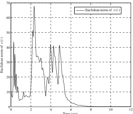
at t=5 (sec). Fig. 4 depicts the state trajectories of master and slave systems. Figs. 5 and 6 show the time responses of synchronization errors and the Euclidean norm of errors vector respectively. It can be seen that the synchronization errors converge to zero after the controllers are activated at t=5 (sec).

6.3 Synchronization Results of Two Rössler and Wang Systems

In this subsection, the parameters of Rössler system

are selected as α=0.25, β = −0.5 and γ =0.05.

More, the parameters of Wang system are considered as

0 2 4 6 8 10 12 14 16 18 20 0

20 40 60 80 100 120

x1

(

t

)

and

xd

(

t

)

Time (sec)

x

1( t )

x

d( t )

Fig. 3 Time response of x t1( )of Wang system which tracks

the desired x td( )=5sin2t.

0 50 100

x1

(

t

) ,

y1

(

t

)

(a)

x₁ (t )

y

1 (t )

-20 0 20

x( 2 t ) , y( 2 t )

(b)

x₂ (t )

y₂ (t )

-40 -20 0 20

x( 3 t ) , y( 3 t )

(c)

x

3 (t )

y

3 (t )

0 2 4 6 8 10 12

-50 0 50

Time (sec) x( 4

t ) , y( 4 t )

(d)

x

4 (t )

y

4 (t )

Fig. 4 Time responses of the state variables of master and

slave Wang systems: (a) Time responses of x t y t₁( ), ( )₁ , (b)

Time responses of x t y t₂( ), ₂( ), (c) Time responses of

3( ), 3( )

x t y t , (d) Time responses of x t y t₄( ), ₄( ).

-40 -20 0 20 40

e1

(

t

)

(a)

e₁ (t )= y₁ (t )- x₁ (t )

-20 0 20

e2

(

t

)

(b)

e

2 (t )= y2 (t )- x2 (t )

-20 0 20

e3

(

t

)

(c)

e

3 (t )= y3 (t )- x3 (t )

0 2 4 6 8 10 12

-40 -20 0 20

Time (sec) e4

(

t

)

(d)

e₄ (t )= y₄ (t )- x₄ (t )

Fig. 5 Synchronization errors between the master and slave

Wang systems: (a) Waveform of e = y_{1 1}‐x₁, (b) Waveform

of e = y_{2 2}‐x₂, (c) Waveform of e = y_{3 3}‐x₃, (d) Waveform

of e = y_{4 4}‐x₄.

0 2 4 6 8 10 12

0 10 20 30 40 50 60 70

Time (sec)

E

u

c

li

d

ean

no

rm

of

e( t )

Euclidean norm of e(t )

Fig. 6 Waveform of the Euclidean norm of synchronization errors vector.

10

a= , b=40, c=2.5, d=10.6, k=1 and h=4 respectively. The initial conditions of master and slave

systems are assumed to be 0 [12, 5, 15, 1.2]

T

= − −

x and

0 [4,8, 13, 2]

T

= − −

y , respectively. Simulation results

are illustrated in Figs. 7-9. The control inputs are

activated at t=5 (sec). Fig. 7 shows the state

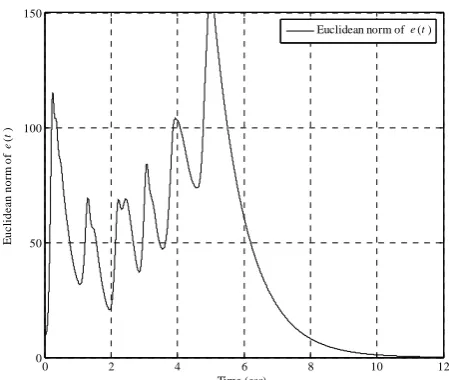
trajectories of master and slave systems. Figs. 8 and 9 show the waveforms of synchronization errors and the Euclidean norm of errors vector. From the Fig. 8, it can be seen that the synchronization errors will converge to zero.

0 50 100

x( 1 t ) , y( 1 t )

(a)

x₁ (t )

y₁ (t )

-20 0 20 40 60

x2

(

t

) ,

y2

(

t

)

(b)

x₂ (t )

y

2 (t )

0 2 4 6 8 10 12

-50 0 50

Time (sec)

x4

(

t

) ,

y4

(

t

)

(d)

x

4 (t )

y₄ (t ) -60

-40 -20 0 20

x3

(

t

) ,

y3

(

t

)

(c)

x₃ (t )

y

3 (t )

Fig. 7 Time responses of the state variables of Wang and

Rössler systems: (a) Time responses of x t y t₁( ), ₁( ), (b) Time

responses of x t y t₂( ), ₂( ), (c) Time responses of x t y t₃( ), ₃( ),

(d) Time responses of x t y t₄( ), ₄( ).

-100 -50 0

e (1 t )

(a)

-50 0 50 100

e (2 t )

(b)

-60 -40 -20 0 20

e (3 t )

(c)

0 2 4 6 8 10 12

-60 -40 -20 0 20

Time (sec)

e (4 t )

(d)

e

1 (t )=y1 (t )- x1 (t )

e

2 (t )=y2 (t )- x2 (t )

e₃ (t )=y₃ (t )- x₃ (t )

e₄ (t )=y₄ (t )- x₄ (t )

Fig. 8 Synchronization errors between the Wang and Rössler

systems: (a) Waveform of e = y_{1 1}‐x₁, (b) Waveform of

2 2 2

e = y ‐x , (c) Waveform of e = y_{3 3}‐x₃, (d) Waveform of

4 4 4

e = y ‐x .

7 Conclusion

An approach for tracking and synchronization problems of hyperchaotic systems using active backstepping method has been proposed in this paper. The mentioned method has been applied to the hyperchaotic Rössler and Wang systems successfully. Three numerical simulations are used to demonstrate the effectiveness of the designed active backstepping controllers.

0 2 4 6 8 10 12

0 50 100 150

Time (sec)

E

u

c

li

d

e

a

n

norm

o

f

e( t )

Euclidean norm of e(t )

Fig. 9 Waveform of the Euclidean norm of synchronization errors vector.

References

[1] Mahmoud E. E., “Dynamics and synchronization

of new hyperchaotic complex Lorenz system”,

Mathematical and Computer Modelling, Vol. 55, No. 7, pp. 1951-1962, Apr. 2012.

[2] Rössler O. E., “An equation for hyperchaos”,

Physics Letters A, Vol. 71: No. 2, pp. 155–157, Apr. 1979.

[3] Pang S. and Liu Y., “A new hyperchaotic system

from the Lü system and its control”, Journal of

Computational and Applied Mathematics, Vol. 235, No. 8, pp. 2775-2789, Feb. 2011.

[4] Yujun N., Xingyuan W., Mingjun W. and

Huaguangv Z., “A new hyperchaotic system and

its circuit implementation”, Communications in

Nonlinear Science and Numerical Simulation, Vol. 15, No. 11, pp. 3518-3524, Nov. 2010.

[5] Liu Y., Yang Q. and Pang G., “A hyperchaotic

system from the Rabinovich system”, Journal of

Computational and Applied Mathematics, Vol. 234, No. 1, pp. 101-113, May. 2010.

[6] Feng C. W., Cai L., Zhang L. S. and Yang X. K.,

“A study on hyperchaotic system implemented by

SETMOS”, Microelectronics Journal, Vol. 42 ,

No. 2, pp. 409-414, Feb. 2011.

[7] Correia M. J. and Rech P. C., “Hyperchaotic

states in the parameter-space”, Applied

Mathematics and Computation, Vol. 218, No. 12, pp. 6711-6715, Feb. 2012.

[8] Haeri M. and Dehghani M., “Modified impulsive

synchronization of hyperchaotic systems”,

Communications in Nonlinear Science and Numerical Simulation, Vol. 15, No. 3, Mar. 2010.

[9] Jawaada W., Noorani M. S. M. and Al-sawalha

M. M., “Robust active sliding mode anti-synchronization of hyperchaotic systems with uncertainties and external disturbances”,

Nonlinear Analysis: Real World Applications, Vol. 13, No. 5, pp. 2403-2413, Oct. 2012.

[10] Hegazi A. S. and Matouk A. E., “Dynamical

behaviours and synchronization in the fractional

order hyperchaotic Chen system”, Applied

Mathematics Letters, Vol. 24, No. 11, pp. 1938-1944, Nov. 2011.

[11] Bai J., Yu Y., Wang S. and Song Y., “Modified

projective synchronization of uncertain fractional

order hyperchaotic systems”, Communications in

Nonlinear Science and Numerical Simulation, Vol. 17, No. 4, pp. 1921-1928, Apr. 2012.

[12] Mahmoud G. M. and Mahmoud E. E.,

“Synchronization and control of hyperchaotic

complex Lorenz system”, Mathematics and

Computers in Simulation, Vol. 80, No. 12, pp. 2286-2296, Aug. 2010.

[13] Kharel R., Busawonand K. and Ghassemlooy Z.,

“A Chaos-Based Communication Scheme Using Proportional and Proportional-Integral

Observers”, Iranian Journal of Electrical and

Electronic Engineering, Vol. 4, No. 4, pp. 127-139, Oct. 2008.

[14] Sundarapandian V., “Hybrid synchronization of

hyperchaotic Rössler and hyperchaotic Lorenz

systems by active control”, International Journal

of Advances in Science and Technology, Vol. 2, No. 4, pp. 1-10, Apr. 2011.

[15] Wu X., Wang H. and Lu H., “Modified

generalized projective synchronization of a new fractional-order hyperchaotic system and its

application to secure communication”, Nonlinear

Analysis: Real World Applications, Vol. 13, No. 3, pp. 1441-1450, Jun. 2012.

[16] Smaoui N., Karouma A. and Zribi M., “Secure

communications based on the synchronization of the hyperchaotic Chen and the unified chaotic

systems”, Communications in Nonlinear Science

and Numerical Simulation, Vol. 16, No. 8, pp. 3279-3293, Aug. 2011.

[17] Shaerbaf S. and Seyedin S. A., “Nonlinear

multiuser receiver for optimized chaos-based

DS-CDMA systems”, Iranian Journal of Electrical

and Electronic Engineering, Vol. 7, No. 3, pp. 149-160, Sep. 2011.

[18] Zhu C., “A novel image encryption scheme based

on improved hyperchaotic sequences”, Optics

Communications, Vol. 285, No. 1, pp. 29-37, Jan. 2012.

[19] Mohammadi S., Talebi S. and Hakimi A., “Two

novel chaos-based algorithms for image and

video watermarking”, Iranian Journal of

Electrical and Electronic Engineering, Vol. 8, No. 2, pp.97-107, Jun. 2012.

[20] Banerjee S., Mukhopadhyay S. and Rondoni L.,

“Multi-image encryption based on synchronization of chaotic lasers and iris

authentication”, Optics and Lasers in

Engineering, Vol. 50, No. 7, pp. 950-957, Jul. 2012.

[21] Banerjee S., Rondoni L. and Mukhopadhyay S.,

“Synchronization of time delayed semiconductor lasers and its applications in digital

cryptography”, Optic Communications, Vol. 284,

No. 19, pp. 4623-4634, Sep. 2011.

[22] Li X. F., Leung A. C. S., Liu X. J., Han X. P. and

Chu Y. D., “Adaptive synchronization of identical chaotic and hyperchaotic systems with

uncertain parameters”, Nonlinear Analysis: Real

World Applications, Vol. 11, No. 4, pp. 2215-2223, Aug. 2010.

[23] Zhang H., Liao X. and Yu J., “Fuzzy modeling

and synchronization of hyperchaotic systems”,

Chaos, Solitons and Fractals, Vol. 26, No. 3, pp. 835-843. Nov. 2005.

[24] Qiaoping L., Rui D. and Bo L., “Hybrid

synchronization of Lü hyperchaotic system with

disturbance by sliding mode control”, Procedia

Engineering, Vol. 15, No. 1, pp. 23-27, Dec. 2011.

[25] Li H. Y. and Hu Y. A., “Robust sliding- mode

backstepping design for synchronization control of cross-strict feedback hyperchaotic systems

with unmatched uncertainties”, Communications

in Nonlinear Science and Numerical Simulation, Vol. 16, No. 10, pp. 3904-3913, Oct. 2011.

[26] Wang J., Gao J. and Ma X., “Synchronization

control of cross-strict feedback hyperchaotic system based on cross active backstepping

design”, Physics Letters A, Vol. 369, No. 5, pp.

452-457, Oct. 2007.

[27] Huang L., Wang M. and Feng R.,

“Synchronization of generalized Henon map via

backstepping design”, Chaos, Solitons and

Fractals, Vol. 23, No. 2, pp. 617-620, Jan. 2005.

[28] Vincent U. E., Ucar A., Laoye J. A. and Kareem

S. O., “Control and synchronization of chaos in RCL-shunted Josephson junction using

backstepping design”, Physica C:

Superconductivity, Vol. 468 , No. 5, pp. 374-382, Mar. 2008.

[29] Laoye J. A., Vincent U. E. and Kareem S. O.,

“Chaos control of 4D chaotic systems using recursive backstepping nonlinear controller”,

Chaos, Solitons and Fractals, Vol. 39, No. 1, pp. 356-362, Jan. 2009.

[30] Harb A. M., Zaher A. A., Al-Qaisia A. A. and

Zohdy M. A., “Recursive backstepping control of

chaotic Duffing oscillators”, Chaos, Solitons and

Fractals, Vol. 34, No. 2, pp. 639-645, Oct. 2007.

[31] Qiang W. F. and Xin L. C., “Hyperchaos evolved

from the Liu chaotic system”, Chinese Physics B,

Vol. 15, No. 5, pp. 963-968, May. 2006.

[32] Liu C., Liu T., Liu L. and Liu K., “A new chaotic

attractor”, Chaos, Solitons and Fractals, Vol. 22, No. 5, pp. 1031-1038, Dec. 2004.

[33] Dou F. Q., Sun J. A., Duan W. S. and Lü K. P., “Controlling hyperchaos in the new hyperchaotic

system”, Communications in Nonlinear Science

and Numerical Simulation, Vol. 14, No. 2, pp. 552-559, Feb. 2009.

Ali Abooee received B.S. and M.S. degrees in electrical engineering from Iran University of Science and Technology (IUST) in 2007 and 2010 respectively. His research interests include chaos and hyperchaos control, nonlinear and robust control.

Mohammad Reza Jahed-Motlagh was born in Tehran, Iran in 1955. He received the B.S. degree in Electrical Engineering from Sharif University of Technology in 1978. He received the M.S. and Ph.D. degree both in Control Theory and Control Engineering from University of Bradford, UK. in 1986 and 1990 respectively. Dr. Jahed-Motlagh is currently an Associate Professor in the Department of Computer Engineering, Iran University of Science and Technology, Tehran, Iran. His main research interests and publications are in the areas nonlinear control, hybrid control systems, multivariable control, chaos computing, and chaos control.