Gold - Silver Nexus: A Threshold Cointegration Approach

Issues

ISSN: 2146-4138

available at http: www.econjournals.com

International Journal of Economics and Financial Issues, 2018, 8(5), 210-219.

Gold - Silver Nexus: A Threshold Cointegration Approach

Zouheir Ahmed Mighri

_{*, Majid Ibrahim Al Saggaf}

1_{Department of Finance and Insurance, College of Business, University of Jeddah, Saudi Arabia,}2_{Department of Finance and}

Insurance, College of Business, University of Jeddah, Saudi Arabia.*Email: [email protected]

ABSTRACT

We investigate the dynamic relationship between the gold and silver prices using the Enders-Siklos threshold cointegration approach. Our data are the weekly prices of the gold and silver from January 1968 to May 2016. We find a, asymmetric threshold cointegration between these two series, instead of the linear cointegration well established in the literature. The short-term adjustment to the equilibrium shows an asymmetric effect according to the price deviation from the long-run equilibrium. Moreover, using an equilibrium adjustment path asymmetry test, we find that, in the short term, gold has a much faster reaction to negative deviations from long-term equilibrium than positive deviations.

Keywords: Threshold Cointegration, Price Transmission, Gold, Silver

JEL Classifications: C13, C22, C32, C52, C53, G15.

1. INTRODUCTION

Precious metals such as gold and silver are strategic commodities whose prices have received much attention. They have been used as a store of value and currency for thousands of years, suggesting that there is a long-run relationship between the two precious

metals (Baur and Tran, 2014). However, several factors may drive

their prices away from each other, namely the industrial demand for silver and jewelery, and the dental demand and central bank demand for gold1_.

The recent popularity of commodities as an investment and a hedge

(Capie et al., 2005; Levin and Wright, 2006; Baur and Lucey, 2010; Baur and McDermott, 2010) against adverse financial or economic

events may constitute an additional force that either creates an otherwise non-existent long-run relationship or strengthens a

preexisting long-run relationship (Batten et al., 2013).

The commodity markets are broadly characterized by movements in their prices that naturally depend on a number of exogenous and endogenous factors. These movements may be upwards or downwards in response to changes in the predictors. Escribano

and Granger (1998) analyzed the relationship between gold and

1 For more details, see World Gold Council (www.gold.org).

silver prices and found that gold and silver are co-integrated mainly

due to a specific bubble and post-bubble period. However, the

magnitude of positive and negative responses may differ for similar positive and negative variations in the predictors, in which case the variables display asymmetric adjustment over the business cycle.

Cointegration and causality analyses are broadly used by some studies to investigate the interdependence and the long-run cointegration relationships between gold and silver prices. Most of these studies either use data that make a comparison with the

Escribano and Granger (1998) study either impossible or analyze

samples that are too short to answer the questions raised by the

authors (Adrangi et al., 2000; Ciner, 2001; Lucey and Tully, 2006; Liu and Chou, 2003; Hammoudeh et al., 2010; Baur and Tran, 2014; Kucher and McCloskey, 2017; Eryiğit, 2017).

The standard cointegration analysis (Engle and Granger, 1987)

assumes that the adjustment mechanism of the error correction

term is symmetric. This indicates that the adjustment coefficients

are the same no matter if the equilibrium error is positive or negative. That is, the adjustment speed of prices is the same regardless of the kind of shocks. Nevertheless, using positive and

negative error terms to denote the positive returns (good news) and negative returns (bad news), the adjustment speed of prices may

The present empirical study contributes significantly to this field of research because, first of all, by using the threshold cointegration test of Enders and Siklos (2001), it determines whether long-run

asymmetric equilibrium relationship between gold and silver prices exists or not. Secondly, to the best of our knowledge, this

study is the first of its kind to utilize the asymmetric threshold

cointegration approach and provides support for asymmetric adjustment behaviour between gold and silver prices. To be

specific, the adjustment coefficient of the error correction term

is different when the equilibrium error is positive from when it is negative.

This paper is organized as follows. Section 2 discusses the econometric methodology. Section 3 outlines the empirical results and section 4 concludes the paper.

2. ECONOMETRIC METHODOLOGY

Cointegration has been widely used to investigate relationship among price variables. The two major cointegration methods are Johansen and Engle-Granger two-step approaches. Both of them assume symmetric relationship between variables. In recent years, threshold cointegration has been increasingly used in price

transmission studies. Balke and Fomby (1997) propose a two-step

approach for examining threshold cointegration on the basis of

the approach developed by Engle and Granger (1987). Enders and Granger (1998) and Enders and Siklos (2001) further generalize

the standard Dickey-Fuller test by allowing for the possibility of asymmetric movements in time-series data. This makes it possible to test for cointegration without maintaining the assumption of a symmetric adjustment to a long-term equilibrium. Thereafter, the method has been widely applied to analyze asymmetric price transmission.

2.1. The Cointegration Approach

Econometric literature proposes different methodological alternatives to empirically analyze the long-run relationships and dynamics interactions between two or more time-series variables. The most widely used methods include the two-step procedure

of Engle and Granger (1987) and the full information maximum likelihood-based approach due to Johansen (1988) and Johansen and Juselius (1990). The first step of the analysis consists in determining a break point into the (Engle and Granger, 1987) relationship that defines the long run relationship between the

gold and silver prices:

Y_1t = ξ₀+ξ₁Y_2t+ε_t (1)

Where Y_1t and Y_2t denote the gold and silver prices, respectively;

ξ0 and ξ1 are parameters to be estimated, and εt is the disturbance

term, which should be stationary if any long-run relationship exists between the two integrated price series.

The parameter ξ1 indicates the long-run elasticity of price

transmission and gives the magnitude of adjustment of the price of gold to variations of the silver price. If ξ1<1, changes in the silver price are not fully passed onto the gold price. Stock (1987) shows

that if variables Y_1t and Y_2t are cointegrated, then the OLS estimates

of ξ0 and ξ1 are super-consistent, and the speed of convergence is

faster than that of stationary variables.

2.2. Modeling Asymmetries in Price Transmission within a Cointegration Framework

The standard approach of Engle and Granger (1987) assumes that

ε_t from Eq. (1) behave as an auto-regressive process in the form of:

1 1

p

t t i t i t

i

z

ε ρε₋ ϕ ε₋

=

∆ = +

∑

Where ρ measures the speed of convergence of the system, z_t is a white-noise disturbance and the residuals from the regression

model are used to estimate ∆ε_t.

Rejecting the null hypothesis of no cointegration ρ=0 in favor of the alternative hypothesis -2<ρ<0 implies that the {ε_t} sequence is stationary with mean zero. Any deviations from the long-run value of the disturbance term ε_t are ultimately eliminated. Convergence is assured if -2<ρ<0. As such, Eq. (1) is an attractor such that ε_t can be written as an error correction model. The change in ε_t equals ρ

multiplied by εt−1 regardless of whether εt−1≥0 or εt−1<0.

Nevertheless, the implicit assumption of linear and symmetric

adjustment is problematic. Enders and Siklos (2001) argue

that the Engle-Granger cointegration test is likely to lead to

misspecification errors when the adjustment of the error correction

term is asymmetric. They remedy this error by expanding the Engle-Granger two-step cointegration test to incorporate an asymmetric error correction term. In the third step, we determine whether or not the disturbance term εt is stationary by considering

an asymmetric test methodology in the form of threshold

autoregressive (TAR) cointegration model as proposed by Enders and Granger (1998) and Enders and Siklos (2001):

∆ε_t= I_t ρ₁ (ε_t-1-τ)+(1-I_t) ρ₂ (ε_t−1-τ)+µ_t (3) Where ρ1, ρ2 are coefficients, τ is the value of the threshold, μt is a

white-noise disturbance and I_t is the Heaviside indicator such that

1 1 1 0

t t

t

if I

if

ε τ

ε τ

−

−

≥ 

=  _<

 (4)

In order for {ε_t} to be stationary, a necessary condition is −2<(ρ1, ρ2)<0. If the variance of μt is sufficiently large, it is also possible

for one value of ρ_j to be in the range of −2 and and for the other

value to equal zero. Although there is no convergence in the regime

with the unit-root (i.e., the regime in which ρ_j=0), large realizations of μ_t will switch the system into the convergent regime.

In both cases, under the null assumption of no cointegration between the variables, the F-statistic for the null hypothesis

adjustment is ρ2 (εt−1-τ) if. If −1<|ρ1|<|ρ2|<0, negative discrepancies

will be more persistent than positive discrepancies. Moreover,

Tong (1983) showed that the OLS estimates of ρ₁ and ρ₂ have an

asymptotic multivariate normal distribution if the sequence {ε_t}

is stationary. Therefore, if the null assumption ρ1=ρ2=0 is rejected, it is possible to test for symmetric adjustment (i.e., ρ1=ρ2) using a standard F-test. Rejecting both the null assumptions ρ₁=ρ₂=0 and ρ1=ρ2 indicates the existence of threshold cointegration and

asymmetric adjustment.

Since the exact nature of the nonlinearity may not be known,

Enders and Siklos (2001) consider another kind of asymmetric

cointegration test methodology that allows the adjustment to be

contingent on the change in εt−1 (i.e., ∆.t−1) instead of the level of εt−1. In this case, the Heaviside indicator of Eq. (4) becomes

1 1 1 0 t

t t if I if ε τ

ε−₋ τ

∆ ≥



=  _{∆ <}

 (5)

Enders and Granger (1998), Enders and Siklos (2001), Kuo and Enders (2004) and Thompson (2006), among others, argue that this specification is especially relevant when the adjustment is such

that the series exhibits more ‘momentum’ in one direction than in the other. That is, the speed of adjustment depends on whether

ε_t is increasing (i.e., widening) or decreasing (i.e., narrowing). According to Thompson (2006), among others, if |ρ1|<|ρ2|, then increase in ε_t tend to persist, whereas decreases revert back to the threshold quickly. The resulting model is called

momentum-TAR (M-momentum-TAR) cointegration model. The momentum-TAR model captures

asymmetrically deep movements if, for instance, positive deviations are more prolonged than negative deviations. The

M-TAR model allows the autoregressive decay to depend on ∆ε_t−1. As such, the M-TAR specification can capture asymmetrically “sharp” movements in {ε_t} sequence (Caner and Hansen, 2001).

In both the TAR and M-TAR cointegration processes, the null

assumption of ρ1=ρ2=0 could be tested, while the null hypothesis of symmetric adjustment may be tested by the restriction, ρ₁=ρ₂. Generally, there is no presumption to whether to use TAR or

M-TAR specifications. Thus, it is recommended to select the

adjustment mechanism by a model selection criterion such as AIC

or SBC. Furthermore, if the errors in Eq. (3) are serially correlated,

it is possible to use the augmented form of the test:

(

) (

) (

)

1 1 1 2 1 ₁

p

t It t It t _i i t i vt

ε ρ ε₋ τ ρ ε₋ τ δ ε ₋

=

∆ = − + − − +

∑

To use the tests, we first regress ε_t on a constant and call the residuals {ˆ }_t , which are the estimates of (ε_t−1-τ). In a second step, we set the indicator according to Eq. (4) or Eq. (5) and estimate

the following regression:

(

)

(

)

(

)

1 1 2 1 ₁

ˆ_{t t} ˆ_t 1 _t ˆ_t p _i ˆ_{t i t}

i

I I v

ε ρ ε₋ τ ρ ε₋ τ δ ε ₋

=

∆ = − + − − +

∑

The number of lags ρ is specified to account serially correlated residuals and it can be selected using AIC, BIC, or Ljung-Box Q test.

In several applications, there is no reason to expect the threshold to

correspond with the attractor (i.e., τ=0). In such circumstances, it is necessary to estimate the value of τ along with the values of ρ1 and ρ2. A consistent estimate of the threshold τ can be obtained by adopting the methodology of Chan (1993). A super consistent estimate of

the threshold value can be attained with several steps. First, the process involves sorting in ascending order the threshold variable, i.e., εˆt−1 for the TAR model or the for the M-TAR model. Second, the potential threshold values are determined. If the threshold value is to be meaningful, the threshold variable must actually cross the

threshold value (Enders, 2004). Thus, the threshold value τ should lie

between the maximum and minimum values of the threshold variable.

In practice, the highest and lowest 15% of the values were removed

from the search to ensure an adequate number of observations on

each side. The middle 70% values of the sorted threshold variable are

used as potential threshold values. Third, the TAR or M-TAR model is estimated with each potential threshold value. The sum of squared errors for each trial can be calculated and the relationship between the sum of squared errors and the threshold value can be examined. Finally, the threshold value yielding the lowest sum of squared errors is deemed to be the consistent estimate of the threshold.

Given these considerations, a total of four models are used in

this study. They are TAR- Eq. (4) with τ=0; consistent TAR- Eq. (4) with τ estimated; MTAR- Eq. (5) with τ=0; and consistent MTAR- Eq. (5) with τ estimated. Since there is generally no presumption on which specification is used, it is recommended to

choose the appropriate adjustment mechanism via model selection

criteria of AIC and BIC (Enders and Siklos, 2001). A model with

the lowest AIC and BIC will be used for further analysis.

Insights into the asymmetric adjustments in the context of a long term cointegration relationship can be obtained with two tests. First, an F-test is used to examine the null assumption of no

cointegration (H0: ρ1=ρ2=0)2 against the alternative of cointegration with either TAR or M-TAR threshold adjustment. Let Φ and Φ* denote the F-statistics for testing the null assumption of ρ1=ρ2=0 under the TAR and the M-TAR specifications, respectively. The distributions of Φ and Φ* are determined by the form of the

attractor. The second one is a standard F-test to assess the null assumption of symmetric adjustment in the long-term equilibrium

(H0: ρ1=ρ2). Rejection of the null hypothesis indicates the existence

of an asymmetric adjustment process.

2.3. Asymmetric Error Correction Model with Threshold Cointegration

The equilibrium correction specification (ECM) of Engle and Granger (1987) assumes that the adjustment process due to

disequilibrium among the variables is symmetric. In order to incorporate asymmetries, two extensions on the ECM model

have been made. Error correction terms and first differences on

the variables are decomposed into positive and negative values,

as proposed by Granger and Lee (1989). The second extension

adds the threshold cointegration mechanism to the Granger and

Lee (1989) approach. The resulting asymmetric error correction

model with threshold cointegration has the form:

1 1

1, 1, 2,

1 1 1

2, 1 Ä + + − − − − + + − − + + − − − = = = − − − = ∆ = + + + + ∆ + ∆ + ∆ +

∑

∑

∑

∑

kt k k t k t

J J J

kj t j kj t j kj t j

j j j

J

kj t j kt j

Y Z Z

Y Y Y

Y

θ δ δ

α α β

β ν (8)

Where k

_{{ }}

− = − − = − −

=

The Heaviside indicator function is constructed from Eq. (4) or Eq. (6).

The superscripts “+” and “-” indicate that the variables are split into

positive and negative components. The first differences are defined as

{

}

, , ,0

+

− −

∆Y_{k t i}=max Y∆ _{k t i (9)}

{

}

, , ,0

−

− −

∆Y_{k t i}=min Y∆ _{k t i} (10)

The lag J is specified to account serially correlated residuals and is selected using AIC statistic and Ljung-Box Q test. The above specification is able to distinguish between long-run and

short-run adjustments of Y_k,t. The long-run adjustment is determined by the parameters _k+ _and

k

−_{, whereas, the short-run adjustment is}

governed by the parameters α α βkj+, kj−, kj+ and for j = 1,…,J and

k = {1,2}. If Y_k,t exhibits asymmetry in long-run adjustment. If either _kj+ _≠_kj− _or

kj kj

+ _≠− _{or both, Y}

k,t displays asymmetry in

short-run adjustment.

In this paper, four types of single or joint null hypotheses and

F-tests are examined (Meyer and Von Cramon-Taubadel, 2004; Frey and Manera, 2007; Sun, 2011). The first type is the Granger

causality test to examine the lead-lag relationship between Y1,t and

Y2,t. The null hypothesis that Y1,t does not lead Y2,t can be tested by

restricting H_01:α₂+_{j =}α₂−_{j =0 for all lags j simultaneously and}

then employing an F-test. Similarly, the null hypothesis that Y2,t

does not lead Y1,t can be tested by restricting H02:β1j β1j 0

+ ₌ − _{= for}

all lags simultaneously and then employing an F-test. The second type of hypothesis is concerned with the distributed lag asymmetric effect on its own variable Y_k,t; that is, H₀₁:α₂+j =α₂−j=0 and H04:β2+j =β2−j =0. The third type of null hypothesis is

the cumulative symmetric effect which can be expressed as

05: ₁ 1 ₁ 1

J J

j j

j j

H α+ α−

= = =

∑

∑

∑

∑

and for Y_2,t. Finally, the equilibrium adjustment path asymmetry can be examined with the null hypothesis of H₀₇:k+=k− to

examine whether it is possible to get back to equilibrium after a shock, and if it is the case, how long it will take.

3. EMPIRICAL RESULTS

This paper focuses on monthly values of the gold and silver prices in US dollars. The sample period runs from January 31, 1968 to

May 31, 2016, with a total of 581 monthly observations obtained for each variable. The data are from the London Bullion Market

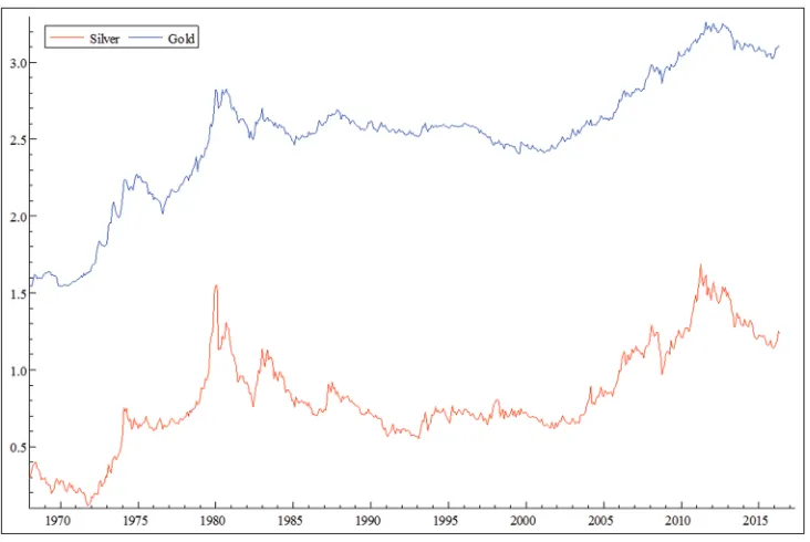
Association. All price series are transformed into natural logarithms. Figure 1 displays the time series plots for the two indices after the logarithm transformation. Generally, gold and silver have an evident comovement, which reveals a high possibility of cointegration between these two series. Although gold and silver prices move together most of the time during our sample period, they also display divergent movement indicating possible nonlinear cointegration. This time-varying comovement may not be detected when the standard linear cointegration model is used, implying that there is a

need to try nonlinear cointegration (Balke and Fomby, 1997; Siklos and Granger, 1997). The plot of the silver is located below that of

the gold, suggesting a price premium in the gold prices.

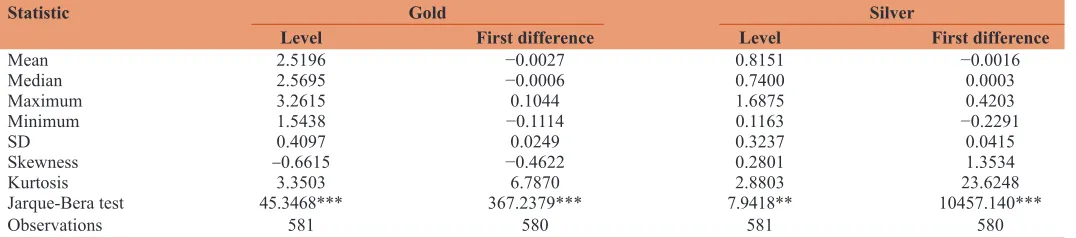
Some summary statistics about these two series are reported in Table 1. We find that the average price of the gold (2.5196) is slightly higher than that of the silver (0.8151), confirming what we

saw in Figure 1. The standard deviation of the prices of the gold

(0.4097) is also higher than that of the silver (0.3237), indicating

a higher volatility in the gold market price. The correlation

coefficient of the gold and silver, which is not reported in Table 1,

is 0.9109, indicating a strong correlation between these two series.

3.2. Results of the Unit Root Test

Before the cointegration analysis, we first examine whether each of the gold and silver price series is an I(1) process or not. The augmented Dickey-Fuller (ADF) test (Dickey, and Fuller, 1979) and Phillips-Perron (PP) test (Phillips and Perron, 1988)

are used to examine the nonstationarity properties of these two series. Results are given in Table 2. For both tests, three

Table 1: Summary statistics for gold and silver prices

Statistic Gold Silver

Level First difference Level First difference

Mean 2.5196 −0.0027 0.8151 −0.0016

Median 2.5695 −0.0006 0.7400 0.0003

Maximum 3.2615 0.1044 1.6875 0.4203

Minimum 1.5438 −0.1114 0.1163 −0.2291

SD 0.4097 0.0249 0.3237 0.0415

Skewness ‑0.6615 −0.4622 0.2801 1.3534

Kurtosis 3.3503 6.7870 2.8803 23.6248

Jarque-Bera test 45.3468*** 367.2379*** 7.9418** 10457.140***

Observations 581 580 581 580

different models are considered: Model without constant, nor deterministic trend, model with constant, without deterministic trend and Model with constant and deterministic trend. The test results are summarized in Table 3. All the test statistics as well as the corresponding P-values reveal that the null hypothesis of the

unit root test cannot be rejected at the 1% significance level or

better for the level forms of the log-transformed gold and silver

price series, but rejected for their first-order differences at the 1% significance level or better. Therefore, both log-transformed

gold and silver prices are integrated processes of order one, or unit root processes.

3.3. Results of the Linear Cointegration Analysis

Table 4 reports the estimated coefficients (ξ0 and ξ1) of the cointegrating vector for each series. We find that the estimated

coefficients of the cointegrating vector are all statistically

significant at the 1% or 5% levels.

Table 2 presents the results from the application of the

Engle-Granger procedure to Eq. (1) with the lag length selected using the

AIC. We include a number of lags enough to remove dependence or serial correlation in the residuals. These test results indicate that the null of no cointegration cannot be accepted.

3.4. Results of the Threshold Cointegration Analysis

From the Engle-Granger ADF cointegration test, the price transmission mechanism may be asymmetric. To investigate this possibility, it is necessary to go further than the usual concept of cointegration in order to allow for asymmetric cointegration and thus asymmetric price transmission.

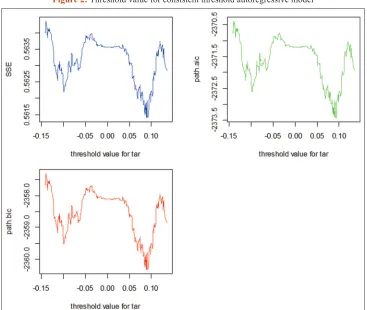
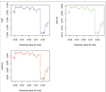
We conduct a nonlinear cointegration analysis by using the TAR models. A total of four models are considered in this study. They

are TAR with τ=0, consistent TAR with τ estimated, MTAR with τ=0 and consistent MTAR with τ estimated (Figures 2 and 3).

Figure 1: Gold and silver after the logarithm transformation.

Table 2: Estimated adjustment equations using the standard engle-granger ADF cointegration and the threshold cointegration tests

Item Engle-granger TAR C.TAR MTAR C.MTAR

Lags (p) 1 6 6 6 6

Threshold (τ) - 0 0.09 0 0.021

ρ1 −0.03*** [−3.014] −0.037*** [−2.637] −0.045*** [−3.061] −0.035** [−2.385] 0.023 [1.143]

ρ2 - −0.016 [−1.117] −0.011 [−0.799] −0.019 [−1.366] −0.043*** [−3.716]

total obs - 581 581 581 581

coint obs - 574 574 574 574

AIC −2365.951 −2346.136 −2347.995 −2345.59 −2353.254

BIC −2352.856 −2306.962 −2308.822 −2306.416 −2314.08

QLB (4) 0.623 0.999 0.999 0.998 0.976

QLB (8) 0.064 0.969 0.971 0.971 0.884

QLB (12) 0.131 0.954 0.951 0.947 0.931

no CI: Φ(H0:ρ1=ρ2=0) - 4.02** (0.0185) 4.951*** (0.0074) 3.747** (0.0242) 7.601*** (0.0006)

no APT: F (H0:ρ1=ρ2) - 1.13 (0.288) 2.97* (0.085) 0.591 (0.442) 8.206*** (0.004)

The notation P is the lag periods of lagged difference term, which is decided by the minimum AIC. The Φ-statistic for the null hypothesis ρ1=ρ2=0 is the threshold cointegration test. It

follows a nonstandard distribution with the critical values are calculated following Enders and Siklos (2001). The F-statistic for the null hypothesis ρ1=ρ2 with two variables in symmetry adjustment follows a standard F distribution. The numbers in the brackets are t-statistics. The numbers in parentheses are P values. ***,_{** and * indicate significance at the 1%, 5% and}

10% levels, respectively. The lag order with the smallest AIC or BIC value is selected. QLB (p) denotes the significance level for the Ljung-Box Q statistic, which tests serial correlation

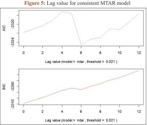
To address possible serial correlation in the residual series, we select an appropriate lag by specifying a maximum lag of 12 (Figures 4 and 5). We use AIC, BIC and Ljung-Box Q statistics

for diagnostic analyses on the residuals. In most cases, the value of the threshold is unknown and has to be estimated along the

values of ρ1 and ρ2. We follow the Chan’s (1993) method to

estimate the threshold values for consistent TAR and M-TAR models.

Table 2 illustrates the results of the threshold cointegration tests using TAR, consistent TAR, MTAR and consistent M-TAR

models. The τ value is the optimal threshold for the indicator

function. Under these conditions, the null hypothesis of threshold

cointegration (ρ₁=ρ₂=0) is rejected. This means that there exists a

cointegrating relationship between gold and silver prices.

Since these price series are cointegrated, we examine whether

their adjustment coefficients are different across positive and

negative errors. This procedure is achieved by verifying the existence of an asymmetric cointegration, i.e., testing the null

assumption of ρ₁=ρ₂. Notice that the asymmetry test only makes sense when the two previous tests reject the null hypothesis. That

is, if the ρi coefficients estimated for the threshold are significantly

different from zero, then the regression is nontrivial and testing for symmetry makes all the sense. As shown in Table 2, we

Figure 2: Threshold value for consistent threshold autoregressive model

Table 3: Unit root test results for gold and silver price series

Statistic Gold Silver

Level First difference Level First difference

t-Stat Lag t-Stat Lag t-Stat Lag t-Stat Lag

ADF (no drift and trend) 2.2498 (0.9945) 0 −22.9301*** (0.0000) 0 0.2578 (0.7606) 0 −24.0503*** (0.0000) 0

ADF (drift) −1.9647 (0.3027) 0 −23.1676*** (0.0000) 0 −1.6910 (0.4354) 0 −24.0647*** (0.0000) 0

ADF (drift and trend) −1.8968 (0.6549) 0 −23.1965*** (0.0000) 0 −2.1749 (0.5022) 0 −24.0446*** (0.0000) 0 PP (no drift and trend) 2.1345 (0.9925) 6 −22.9927*** (0.0000) 7 0.2707 (0.7642) 4 −24.0513*** (0.0000) 4

PP (drfift) −1.9472 (0.3106) 6 −23.1788*** (0.0000) 6 −1.6832 (0.4393) 3 −24.0662*** (0.0000) 4

PP (drift and trend) −1.9337 (0.6354) 6 −23.2031*** (0.0000) 6 −2.1886 (0.4946) 2 −24.0459*** (0.0000) 4 Entries are unit root test statistics with the corresponding P values in parentheses. ADF denotes the ADF test (Dickey, and Fuller, 1979) and PP denotes the Phillips and Perron test (Phillips and Perron, 1988). For the ADF test, the optimal lags are determined by Schwarz Information Criterion (SIC). For the PP test, we adopt Bartlett kernel using Newey-West

bandwidth. *resp. **,_{***: Rejection of the null hypothesis at the 10% (resp. 5%, 1%) significance level}

Table 4: The estimated long-run equilibrium relationships

Series ξ0 ξ1

Coefficient P value Coefficient P value

Silver-gold −0.99823*** 0.0000 0.71970*** 0.0000

found evidence of asymmetric price transmission. Therefore, the gold prices became cointegrated with the silver prices, the adjustment mechanism is asymmetric and the speed of adjustment to the equilibrium is different when the last equilibrium error has different signs. This means that the change in the equilibrium error has a different impact on the adjustment speed to the new

equilibrium (Anderson, 1997).

Focusing on the results from the consistent M-TAR model, the -test

for the null hypothesis of no cointegration has a statistic of 7.601 and it is highly significant at the 1% level. Thus, gold and silver

are cointegrated with threshold adjustment. Furthermore, the F statistic for the null hypothesis of symmetric adjustment has a value

of 8.206 and it is also significant at the 1% level. Therefore, the

adjustment process is asymmetric when the gold and silver prices adjust to achieve the long-term equilibrium. The point estimate for

the price adjustment is 0.023 for positive shocks and −0.043 for

negative shocks. Positive deviations from the long-term equilibrium resulting from increases in gold price or increases in silver price

1

(

∆

ε

ˆ

≥

0.021)

deviations from the long-term equilibrium resulting from decreases in the gold price or increases in the silver price

(

∆

ε

ˆ

≥

0.021)

are eliminated at a rate of 4.3% per month. In other words, positive deviations take about 44 months (1/0.023=43.47 months) to be

fully digested while negative deviations take about 24 months

only (1/0.043=23.25 months). Therefore, there is substantially faster convergence for negative (below threshold) deviations from long-term equilibrium than positive (above threshold) deviations.

3.5. Results of the Asymmetric Error Correction Model

In the light of the weight of evidence in support of asymmetric adjustments, an asymmetric error correction model could be used to investigate the movement of the gold and silver price series in a long-run equilibrium relationship. The asymmetric error correction model with threshold cointegration is estimated and the results are reported in Table 5. Diagnostic analyses on the residuals with AIC, BIC and Ljung-Box Q statistics select a lag of four for the models.

Note that the consistent M-TAR model is the best from the threshold cointegration analyses and the error correction terms

Figure 3: Threshold value for consistent MTAR model

are constructed using Eq. (5) and Eq. (7). Results show that

gold is cointegrated with silver and it also exhibits asymmetric

adjustments. In the equation for silver, there are four coefficients

statistically significant at the 5% and 10% levels, respectively,

(i.e. α+

1, β−3, δ+, and δ-). In equation for gold, there are only two

significant coefficients (i.e., α+

3 and δ-). Besides, the short-term

equilibrium adjustment process occurs with both gold and silver

prices since δ+_=δ-_{. Given the case silver price is larger than gold}

price, there are three situations to reduce the price deviations (Chen

et al., 2013): (i) Silver price goes down and gold price goes up; (ii) silver price goes down and gold price goes down as well, but silver price drops more; (iii) silver price goes up and gold price

goes up, but silver price increases less.

In our empirical findings, for regimes with positive shocks (silver price is higher than gold price), the adjustment coefficient for silver is 0.033 and 0.036 for gold, which means that, in the next

period, gold price will go up and silver price will go down, thus, the price deviation will decrease. For regimes with negative shocks

(silver price is lower than gold price), the adjustment coefficient for silver is −0.017 and −0.067 for gold, which means that, in the

next period, gold price will go down and silver price will go down as well, but gold drops more and thus the price deviation will

decrease. Diagnostic analyses on the residuals with Ljung-Box

Table 5: Results of the asymmetric error-correction models with threshold cointegration

Item Gold-silver (C-MTAR, lag=4)

Silver Gold

Estimate t-Statistic Estimate t-Statistic

Estimate

θ −0.001 −0.515 −0.005 −1.298

α+

1 0.184** 2.086 0.097 0.658

α+

2 −0.039 −0.44 −0.155 −1.047

α+

3 0.073 0.81 0.25* 1.666

α+

4 −0.028 −0.317 −0.006 −0.042

α−

1 −0.133 −1.221 0.09 0.496

α−

2 0.04 0.366 −0.198 −1.09

α−

3 −0.003 −0.026 −0.082 −0.452

α−

4 0.034 0.316 0.058 0.318

β+

1 −0.029 −0.451 −0.025 −0.23

β+

2 −0.042 −0.699 0.092 0.92

β+

3 0.03 0.492 −0.067 −0.67

β+

4 0.016 0.25 0.037 0.346

β−

1 −0.011 −0.194 −0.097 −1.018

β−

2 −0.009 −0.164 0.05 0.56

β−

3 −0.109** −2.055 −0.083 −0.936

β−

4 0.035 0.659 −0.014 −0.16

δ+ _{0.033* 1.843 0.036 1.225}

δ− −0.017* −1.657 −0.067*** −3.923

Hypothesis description

Granger causality test: 0.705 [0.69] 0.826 [0.58]

Granger causality test: 0.742 [0.65] 0.673 [0.72]

Distributed lag asymmetry test: 0.254 [0.62] 0.027 [0.87]

Distributed lag asymmetry test: 0.045 [0.83] 0.114 [0.74]

Cumulative asymmetry test: 0.936 [0.33] 0.542 [0.46]

Cumulative asymmetry test: 0.183 [0.67] 0.468 [0.49]

Equilibrium adjustment path asymmetry test: H₀₇: δ+_=δ- _{6.64*** [0.01] 10.316*** [0.000]}

Diagnostics

R2 _{0.042 - 0.047}

-Adj-R2 _{0.011 - 0.016}

-AIC −2604.716 - −2018.585

-BIC −2517.594 - −1931.463

-LB (4) 0.995 - 0.989

-LB (8) 0.689 - 0.715

-Numbers in brackets are P values. For the hypotheses, H01 and H02 are Granger causality tests, H03 and H04 evaluate distributed lag asymmetric effect, H05 and H06 assess the cumulative asymmetric effect, and H07 is about equilibrium adjustment path asymmetric effect. ***, ** and * denote significance at the 1%, 5%, and 10% levels, respectively

Q statistics select a lag of four for the model. The adjusted-R2 ₌ 0.011 for silver and 0.016 for gold. Moreover, the AIC and BIC

statistics for gold are both larger than those for silver. This means

that the model specification is better fitted on gold.

Using the estimation results of the asymmetric ECM with threshold cointegration, we also conduct the hypothesis testing described in section 2 (paragraph 2.3). The hypotheses of

Granger causality between the series are assessed with F-tests.

The F-statistic of 0.826 reveals that silver does not Granger cause gold. Besides, the F-statistic of 0.742 indicates that gold

does not Granger cause silver. This indicates that, in the short term, both precious metals do not affect each other. Similarly,

the F-statistic of 0.705 for silver discloses that the lagged price series have not significant impacts on its own price. Furthermore, the F-statistic of 0.673 for gold reveals that the lagged price series have no significant impacts on its own price. Thus,

in the short term, silver and gold have been evolving more independently.

Several kinds of assumptions are examined for asymmetric price

transmission. The first one is the distributed lag asymmetric effect.

In each price equation, the equality of the corresponding positive

and negative coefficients for each of the four lags is tested; in total,

there are eight F-tests for this hypothesis. It turns out that none

of them is statistically significant and distributed lag asymmetric

effect does not exist. Furthermore, the cumulative asymmetric

effects are also examined. The largest F-statistic is 0.936 but none of the four statistics are significant at the conventional level. Thus, cumulative effects are symmetric. The final type of

asymmetry examined is the momentum equilibrium adjustment

path asymmetries, which are statistically significant for both gold and silver. For silver, the F-statistic is 6.64 with a P = 0.01. The point estimates of the coefficients for the error correction terms are 0.033 for positive error correction term and −0.017 for the negative one. Besides, for gold, the F-statistic is 10.316 with a P = 0.000. The point estimates are 0.036 with a t-value of 1.225 for positive deviations and −0.067 with a t-value of −3.923 for

negative deviations. The magnitude suggests that, in the short term,

gold responds to the positive deviations by 3.6% in a month but by 6.7% to negative deviations. Measured in response time, positive and negative deviations take, respectively, 27.78 and 14.92 months

to be fully digested. Therefore, in the short term, gold has a much faster reaction to negative deviations from long-term equilibrium than positive deviations.

4. SUMMARY AND CONCLUDING

REMARKS

In this paper, we extended the study by Escribano and Granger

(1998) by using the Enders-Siklos asymmetric threshold

cointegration approach to examine the long-run asymmetric

equilibrium relationships between gold and silver prices for a 47-year period from 1968 to 2016. The asymmetric error correction

models extend the standard cointegration models to deal with the problem of low power of unit roots and cointegration tests in the presence of asymmetric adjustment.

The estimated results are presented in the following. First, when the conventional Engle-Granger symmetric cointegration test is

used, gold and silver prices are cointegrated. Second, we find

that gold and silver prices become cointegrated and are in an asymmetric form, which indicates the existence of an asymmetric effect in the short-term adjustment process. Regimes with negative

(below the threshold) changes of deviations from long-term

equilibrium adjust much quicker than regimes with positive (above

the threshold) changes of deviations. Third, the transmission

mechanism between gold and silver prices has been asymmetric in both the long-term and short-term. Using a Granger causality test,

we do not find a bi-directional causality between these two series,

indicating that gold and silver prices do not affect each other in our sample period. Besides, using an equilibrium adjustment path

asymmetry test, we find that, in the short term, gold has a much

faster reaction to negative deviations from long-term equilibrium than positive deviations.

REFERENCES

Adrangi, B., Chatrath, A., David, R.C. (2000). Price discovery in strategically-linked markets: The case of the gold-silver spread. Applied Financial Economics, 10(3), 227-234.

Anderson, H.M. (1997), Transaction costs and nonlinear adjustment towards equilibrium in the US treasury bill market. Oxford Bulletin of Economics and Statistics, 59, 465-484.

Balke, N.S., Fomby, T.B. (1997), Threshold co integration. International Economic Review 38, 627-645.

Batten, J.A., Ciner, C., Lucey, B., Szilagyi, P. (2013), The structure of gold and silver spread returns. Quantitative Finance, 13 (4), 561-570. Baur, D.G., Lucey, B.M. (2010), Is gold a Hedge or a Safe Haven? An

analysis of stocks, bonds and gold. The Financial Review, 45(2), 217-229.

Baur, D.G., McDermott, T.K. (2010), Is gold a safe haven? International evidence. Journal of Banking and Finance, 34(8), 1886-1898. Baur, D.G., Tran, D.T. (2014), The long-run relationship of gold and

silver and the influence of bubbles and financial crises. Empirical Economics, 47(4), 1525-1541.

Caner, M., Hansen, B. (2001), Threshold auto regression with a unit-root. Econometrica 69, 1555-1596.

Capie, F., Mills, T.C., Wood G. (2005), Gold as a hedge against the dollar. Journal of International Financial Markets Institutions and Money, 15(4), 343-352.

Chan, K.S. (1993), Consistency and limiting distribution of the least squares estimator of a threshold autoregressive model. Annals of Statistics, 21, 520-533.

Chen, H., Choi, P.M.S., Hong, Y. (2013), How smooth is price discovery? Evidence from cross-listed stock trading. Journal of International Money and Finance, 32, 668-699.

Ciner, C. (2001), On the long-run relationship between gold and silver: A note. Global Finance Journal, 12(2), 299-303.

Dickey, D., Fuller, W.A. (1979), Distribution of the estimators for autoregressive time series with a unit root. Journal of the American Statistical Association, 74(366), 427-431.

Enders, W. (2004), Applied Econometric Time Series. New York: John Wiley & Sons, Inc. p480.

Enders, W., Granger, C.W.F. (1998), Unit-root tests and asymmetric adjustment with an example using the term structure of interest rates. Journal of Business and Economic Statistics, 16, 304-311. Enders, W., Siklos, P.L. (2001), Cointegration and threshold adjustment.

Engle, R., Granger, C.W.J. (1987), Cointegration and error correction: Representation, estimation, and testing. Econometrica, 55, 251-276. Eryiğit, M. (2017), Short-term and long-term relationships between gold

prices and precious metal (palladium, silver and platinum) and energy (crude oil and gasoline) prices. Economic Research-Ekonomska Istraživanja, 30 (1), 499-510.

Escribano, A., Granger, C.W. (1998), Investigating the relationship between gold and silver prices. Journal of Forecasting, 17(2), 81-107. Frey, G., Manera, M. (2007), Econometric models of asymmetric price

transmission. Journal of Economic Surveys, 21(2), 349-415. Granger, C.W.J., Lee, T.H. (1989), Investigation of production, sales, and

inventory relationships using multicointegration and non-symmetric error correction models. Journal of Applied Economics, 4, 145-159. Hammoudeh, S., Chen, L.H., Fattouh, B. (2010), Asymmetric adjustments

in oil and metals markets. The Energy Journal, 31(4), 183-203. Johansen, S. (1988), Statistical analysis of cointegration vectors. Journal

of Economic Dynamics and Control, 12, 231-254.

Johansen, S., Juselius, K. (1990), Maximum likelihood estimation and inference on cointegration with applications to the demand for money. Oxford Bulletin of Economics and Statistics, 52, 169-210. Kucher, O., McCloskey, S. (2017), The Long run relationship between

precious metal prices and the business cycle. The Quarterly Review of Economics and Finance, 65, 263-275.

Kuo, S.H., Enders, W. (2004), The term structure of Japanese interest rates: The equilibrium spread with asymmetric dynamics. Journal

of the Japanese and International Economies, 18, 84-98.

Levin, E.R., Wright, R.E. (2006), Short-Run and Long-Run Determinants of the Price of Gold. World Gold Council. Research Study no. 32. Liu, S.M., Chou, C.H. (2003), Parities and spread trading in gold and

silver markets: A fractional co-integration analysis. Applied Financial Economics, 13(12), 899-911.

Lucey, B.M., Tully, E. (2006), The evolving relationship between gold and silver 1978-2003: Evidence from dynamic cointegration analysis. Applied Financial Economics Letters, 2 (1), 47-53.

Meyer, J., Von Cramon-Taubade, S. (2004). Asymmetric price transmission: A survey. Journal of Agricultural Economics, 55(3), 581-611.

Phillips, P.C.B., Perron, P. (1988), Testing for a unit root in time series regression. Biometrika, 75(2), 335-346.

Siklos, P., Granger, C.W. (1997), Regime sensitive cointegration with an application to interest rate parity. Macroeconomic Dynamics, 3, 640-657.

Stock, J. (1987), Asymptotic properties of least-squares estimators of cointegrating vectors. Econometrica, 55, 1035-1056.

Sun, C. (2011), Price dynamics in the import wooden bed market of the United States. Forest Policy and Economics, 13, 479-487.

Thompson, M.A. (2006), Asymmetric adjustment in the prime lending– deposit rate spread. Review of Financial Economics, 15, 323-329. Tong, H. (1983), Threshold Models in Non-Linear Time Series Analysis.