The Thirty-Third AAAI Conference on Artificial Intelligence (AAAI-19)
FRAME Revisited: An Interpretation View Based on Particle Evolution
Xu Cai,
1†Yang Wu,
1†Guanbin Li,
1Ziliang Chen,
1Liang Lin
1,2∗ 1School of Data and Computer Science, Sun Yat-Sen University, China2Dark Matter AI Inc.
[email protected], [email protected], [email protected], [email protected], [email protected]
Abstract
FRAME (Filters, Random fields, And Maximum Entropy) is an energy-based descriptive model that synthesizes visual re-alism by capturing mutual patterns from structural input sig-nals. The maximum likelihood estimation (MLE) is applied by default, yet conventionally causes the unstable training en-ergy that wrecks the generated structures, which remains un-explained. In this paper, we provide a new theoretical insight to analyze FRAME, from a perspective of particle physics ascribing the weird phenomenon to KL-vanishing issue. In order to stabilize the energy dissipation, we propose an al-ternative Wasserstein distance in discrete time based on the conclusion that the Jordan-Kinderlehrer-Otto (JKO) discrete flow approximates KL discrete flow when the time step size tends to0. Besides, this metric can still maintain the model’s statistical consistency. Quantitative and qualitative experi-ments have been respectively conducted on several widely used datasets. The empirical studies have evidenced the ef-fectiveness and superiority of our method.
Introduction
FRAME (Filters, Random fields, And Maximum En-tropy) (Zhu, Wu, and Mumford 1997) is a model built on Markov random field that can be applied to approxi-mate various types of data distributions, such as images, videos, audios and 3D shapes (Lu, Zhu, and Wu 2015; Xie, Zhu, and Wu 2017; Xie et al. 2018). It is an energy-based descriptive model in the sense that besides its pa-rameters are estimated, samples can be synthesized from the probability distribution the model specifies. Such distri-bution is derived from maximum entropy principle (MEP), which is consistent with the statistical properties of the ob-served filter responses. FRAME can be trained via an infor-mation theoretical divergence between real data distribution
∗
Xu Cai and Yang Wu contribute equally to this work and share first-authorship. The corresponding author is Liang Lin (Email: [email protected]). This work was supported in part by the National Key Research and Development Program of China under Grant No.2018YFC0830103, in part by the NSFC-Shenzhen Robotics Projects (U1613211), in part by the National Natural Science Foundation of China under Grant No.61702565, No.61622214 and No.61836012 and in part by National High Level Talents Special Support Plan (Ten Thousand Talents Program).
Copyright c2019, Association for the Advancement of Artificial Intelligence (www.aaai.org). All rights reserved.
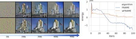
1th 10th 30th 60th 90th
Figure 1: Visual and numerical results of FRAME and wFRAME. Left: the generating steps and selected typical results of “spaceship” from two algorithms. The first and the second-row images are respectively from FRAME and wFRAME. wFRAME achieves higher quality images com-pared with FRAME, which collapses at the very beginning of the sampling iteration. Right: the observed model energy of both algorithms. The instability of the energy curve is the signal of the model collapse. The detailed discussion can be found in the experiment section.
Pr and model distributionPθ. Primitive efforts model it as KL-divergence by default, which also leads to the same re-sults of MLE.
A large number of experimental results reveal that FRAME tends to generate inferior synthesized images and is often arduous to converge during training. For instance, displayed in Fig. 1, the synthesized images of FRAME se-riously deteriorates along with the model energy. This phe-nomenon is caused by KL-vanishing in the stepwise parame-ters estimation of the model due to the existence of the great filter responses disparity between Pθ andPr. Specifically, the MLE-based learning algorithm attempts to optimize a transformation from the high dimensional support ofPθto the non-existing support ofPr, i.e., it starts from an initial-ization of a Gaussian noise covering the whole support of
PθandPr, then gradually updatesθby calculating the KL discrete flow step-wisely. Therefore in the discrete time set-ting of the actual iterative training process, the dissipation of the model energy may become considerably unstable, and the stepwise minimization scheme may suffer serious KL-vanishing issue during the communicative parameters esti-mation.
discrete flow), which helps explore the reasons for the col-lapses of the FRAME model. This is inspired by the fact that the empirical measure of a set of Brownian particles generated byPθ satisfies Large Deviation Principle (LDP) with rate functional coincides exactly with the KL discrete flow (see Lemma 1). We then delve into the model in discrete time state and translate its learning mechanism from KL discrete flow into the Jordan-Kinderlehrer-Otto (JKO) (Jor-dan, Kinderlehrer, and Otto 1998) discrete flow, which is a procedure for finding time-discrete approximations to solu-tions of diffusion equasolu-tions in Wasserstein space. By resort-ing to the geometric distance between Pθ andPr through optimal transport (OT) (Villani 2003) and replacing the KL-divergence with Wasserstein distance (a.k.a. the earth mover’s distance (Rubner, Tomasi, and Guibas 2000)), this method manages to stabilize the energy dissipation scheme in FRAME and maintain its statistical consistency. The whole theoretical contribution can be summed up as the fol-lowing deduction process:
• We deduce the learning process of data density in FRAME model from a view of particle evolution and con-firm that it can be approximated by a discrete flow model with gradually decreasing energy driven by the minimiza-tion of the KL divergence.
• We further propose Wasserstein perspective of FRAME (wFRAME) by reformulating the FRAME’s learning mechanism from KL discrete flow into the JKO discrete flow, of which the former theoretically explains the cause of the vanishing problem, while the latter overcomes the drawbacks, including the instability of sample generation and the failure of model convergence during training.
Qualitative and quantitative experiments demonstrate that the proposed wFRAME greatly ameliorates the vanishing issue of FRAME and can generate more visually promis-ing results, especially for structurally complex trainpromis-ing data. Moreover, to our knowledge, this method can be applied to most sampling processes which aim at abridging the KL-divergence between real data distribution and the generated data distribution by time sequence.
Related Work
Descriptive Model for Generation. The descriptive mod-els originated from statistical physics have an explicit prob-ability distribution of the signal, where they are ordinarily called the Gibbs distributions (Landau and Lifshitz 2013). With the massive developments of Convolutional Neural Networks (CNN) (Krizhevsky, Sutskever, and Hinton 2012) which has been proven to be a powerful discriminator, re-cently, increasing researches on the generative perspective of this model have drawn a lot of attention. (Dai, Lu, and Wu 2014) first introduces a generative gradient for pre-training discriminative ConvNet by a non-parametric impor-tance sampling scheme and (Lu, Zhu, and Wu 2015) pro-poses to learn FRAME using pre-learned filters of modern CNN. (Xie et al. 2016b) further studies the theory of gen-erative ConvNet intensively and show that the model has a
representational structure which can be viewed as a hierar-chical version of the FRAME model.
Implicit Model for Generation. Apart from the descrip-tive models, another popular branch of deep generadescrip-tive mod-els is black-box modmod-els which map the latent variables to signals via a top-down CNN, such as the Generative Ad-versarial Network (GAN) (Goodfellow et al. 2014) and its variants. These models have gained remarkable success in generating realistic images and learn the generator network with an assistant discriminator network.
Relationship. Unlike the majority of implicit generative models, which use an auxiliary network to guide the training of the generator, descriptive models maintain a single model which simultaneously serves as a descriptor and generator, though FRAME can be served as an auxiliary and be com-bined with GAN to facilitate each other (Xie et al. 2016a). They factually generate samples directly from the input set, rather than from the latent space, which to a certain extent ensures that the model can be efficiently trained and produce stable synthesized results with relatively less model struc-ture complexity. In this paper, FRAME and its variants as described above share the same MLE based learning mech-anism, which follows an analysis-by-synthesis scheme and works by first generating synthesized samples from the cur-rent model using Langevin dynamics and then learn the pa-rameters through observed-synthesized samples’ distance.
Preliminaries
Let P denote the space of Borel probability measures on any given subset of space X, where ∀x ∈ X,
x ∈ Rd. Given some sufficient statistics φ : X → R,
scalar α ∈ R and base measure q, the space of distri-butions satisfying linear constraint is defined as Plin
α =
p, f ∈ P:p=f q, f ≥0,R
pdx= 1, Ep[φ(x)] =α . The Wasserstein space of order r ∈ [1,∞] is defined as Pr = p∈ P:R|x|rdp <∞ , where | · |r denotes the
r-norm onX.|X |is the number of elements in domainX. ∇denotes gradient and∇·denotes the divergence operator.
Markov Random Fields (MRF). MRF belongs to the family of undirected graphical models, which can be writ-ten in the Gibbs form as
P(x;θ) = 1
Z(θ)exp
( K
X
k=1
θkfk(x)
)
, (1)
where K stands for the number of features {fk} K k=1 and
Z(·) is the partition function (Koller and Friedman 2009). Its MLE learning process follows the iteration of the follow-ing two steps:
I.Update model parameterθby ascending the gradient of the log likelihood
∂ ∂θk
1
N logP(x;θ) =EPr[fk(x)]−EP(x;θ)[fk(x)], (2)
whereEPr[fk(x)] andEP(x;θ)[fk(x)]is respectively the
II. Sample from the current model by parallel MCMC chains. The sampling process, according to (Younes 1989), does not necessarily converge at eachθt, thus we only estab-lish one persistent sampler that converges globally in order to reduce calculus.
FRAME Model. Based on an energy function, FRAME is defined on the exponential tilting of a reference distribu-tionq, which is a reformulation of MRF and can be written as (Lu, Zhu, and Wu 2015):
P(x;θ) = 1
Z(θ)exp
( K
X
k=1
X
x∈X
θkh(hx,wi+b)k
)
q(x),
(3)
whereh(x) = max(0,x)is the nonlinear activation func-tion,hx,wiis the filtered image or feature map andq(x) =
1
(2πσ2)|X |/2 exp
− 1 2σ2kxk
2
denotes the Gaussian white
noise model with mean0and varianceσ2.
KL Discrete Flow. This flow is related to discrete prob-ability distributions (evolutions discretized in time) with fi-nite dimensional problems. More precisely, it indicates the system ofnindependent Brownian particles{xi}n
i=1 ∈Rd
whose position inRd is given by a Wiener process satisfies the following stochastic differential equation (SDE)
dxt=µ(xt)dt+ε(xt)dBt. (4)
µis the drift term,εstands for the diffusion term,Bdenotes the Wiener process and subscripttdenotes time point. The empirical measure of those particles is proved to approxi-mate Eq. 3 by an implicit descent step ρ∗ = argminρIt, whereIt is the so called KL discrete flow consists of KL divergence and energy functionΦ :Rd →R.
It=K(ρ|ρt) +
Z
Φdρ. (5)
Particle Perspective of FRAME Model
Although there is a traditional statistical perspective to in-terpret the FRAME theory (Xie et al. 2016b), we still need a more stable sampling process to avoid this frequent gen-eration failure. We revisit the FRAME model from a com-pletely new particle perspective and prove that its parameter update mechanism is actually equivalent to the reformula-tion of KL discrete flow. Its further transformareformula-tion, a mech-anism in JKO discrete flow manner which we will next prove the equivalence on condition of enough sampling time steps, has ameliorated this unpredictably vanishing phenomenon. All the proofs in detail are added to Appendix A.
Discrete Flow Driven by KL-divergence
Herein we first introduce FRAME in discrete flow manner. If we regard the observed signals {xi
t}ni=1 with the
gener-ating function of Markov property as Brownian particles, then Theorem 1 points out that Langevin dynamics can be deduced from KL discrete flow sufficiently and necessarily through Lemma 1.
Lemma 1. For i.i.d. particles {xit}ni=1 with common
gen-erating functionE[eΦ(x;θ)]which has Markov property, the
empirical measureρt=n1P n i=1δxi
tsatisfies LDP with rate
functional in the form ofIt.
Theorem 1. Given a base measureq, a clique potentialΦ, the density of FRAME in Eq. 3 can be obtainedsufficiently and necessarilyby solving the following constrained opti-mization.
ρt+1= argmin
ρ
K(ρ|ρt),
s.t.
Z
Φdρ=
Z
ΦdPr, ρ0=q, ∀ρ∈ Pαlin. (6)
Let θ be the Lagrange multiplier integrated in Φ(x;θ) and ensureE[eΦ(x;θ)]<∞, the optimizing objective can be
reformulated as
Il t= min
ρ maxθ
n
K(ρ|ρt) + Z
Φ(x;θ)dρ−
Z
Φ(x;θ)dPr o
. (7)
Since ∇xlogP(x;θ) = ∇xΦ(x;θ), the SDE iteration ofxtin Eq. 4 can be expressed in the Langevin form as
xt+1=xt+∇xlogP(xt;θ) + √
2ξt. (8)
By Lemma 1, if we fix θ, the sampling scheme in Eq. 8 approaches the KL discrete flowIl
t, the flow will fluctuate in caseθ varies. θ is updated by calculating∇θItl, which impliesθcan dynamically transform the transition map into desired. The sampling process of FRAME can be summed up as
xt+1=xt−
xt
σ2− ∇xΦ(xt;θ)
+√2ξt
θt+1=θt+∇θEρt[Φ(x;θ)]− ∇θEPr[Φ(x;θ)],
(9)
where−xt/σ2 is the derivative of initial Gaussian noiseq. If we take a close look at the objective function, there is an adversarial mechanism while updatingxtandθt. Regard-less of fixingθupdatingx, or fixingxupdatingθ, the cor-rect dicor-rection cannot be insured to the optimal of minimizing K(P(x;θ)|Pr).
Discrete Flow Driven by Wasserstein Metric
Fokker-Planck Equation. Under the influence of drifts and random diffusions, this equation describes the evolution of the probability density of the particle velocity. LetF be an integral function andδF/δρ denote its Euler-Lagrange first variation, the equations are
∂tρ+∇ ·(ρν) = 0 (Continuity equation)
ν=−∇δF
δρ (Variational condition) ρ(·,0) =ρ0 ρ0∈L1(Rd), ρ0≥0.
(10)
Wasserstein Metric. The Benamou-Brenier form of this metric (Benamou and Brenier 2000) of order r involves solving a smoothy OT problem over any probabilitiesµ1and
µ2inPrusing the continuity equation showed in Eq. 10 as follows, whereν belongs to the tangent space of the mani-fold governed by some potential and associated with curve
ρt.
Wr(µ
1, µ2) := min
ρt∈Pr {
Z 1
0
Z
Rd
|νt|rdρtdt:∂tρt
+∇ ·(ρt·νt) = 0|ρ0=µ1, ρ1=µ2}.
(11)
JKO Discrete Flow. Following the initial work (Jordan, Kinderlehrer, and Otto 1998), which shows how to re-cover Fokker-Planck diffusions of distributions in Eq. 10 when minimizing entropy functionals according to Wasser-stein metric W2, the JKO discrete flow is applied by our
method to replace the initial KL divergence with the entropic Wasserstein distanceW2−H(ρ). The function of the flow
is
Jt= 1
2W
2(ρ, ρt) +
Z
logρdρ+
Z
Φdρ. (12)
Remark 1. The initial Gaussian termqis left out for con-venience to facilitate the derivation, otherwise, the entropy −H(ρ) =Rlogρdρin Eq. 12 should be written as the rela-tive entropyK(ρ|q).
By Theorem 1,Jtinstead ofItcan be calculated in ap-proximation and its steady state will approach Eq. 3. Apply-ingJtin the manner of dissipation mechanism as a substi-tute ofItallows regarding the diffusion Eq. 4 as the steep-est descent of clique energyΦ and entropy−H(P)w.r.t. Wasserstein metric. Solving such optimization problem us-ing W is identical to solve the Monge-Kantorovich mass transference problem.
With Second Mean Value theorem for definite integrals, we can approximately recover the integralW2by two
ran-domly interpolated rectangles
W2(ρ
t0, ρt1) := inf ρt
Z t1
t0
Z
Rd
|∇Φ|2dρ
tdt
≈(ζ−t0)
Z
Rd
|∇Φ|2dρ
t0+ (t1−ζ)
Z
Rd
|∇Φ|2dρ
t1
=−β
(1−γ)
Z
Rd
|∇Φ|2dρ
t0+γ
Z
Rd
|∇Φ|2dρ
t1
.
(13)
whereβ = t1−t0 parameterizes the time piece andγ =
ζ/β(0≤γ≤1)represents random interpolated parameter
sinceζis random. With Eq. 13, the functional derivative of W2(ρ
t0, ρt1)w.r.t.ρt1is then proportional to
δW2(ρ
t0, ρt1)
δρt1
∝ |∇Φ|2, (14)
which is exactly the result of Proposition 8.5.6 in (Ambro-sio, Gigli, and Savar´e 2008). Assume Φ be at least twice differentiable and treat Eq. 14 as the variational condition in Eq. 10, then plug Eq. 14 into the continuity equation of Eq. 10, which turns into a modified Wasserstein gradient flow in Fokker-Planck form as follows
∂tρ= ∆ρ−∇ · ρ(∇Φ− ∇|∇Φ(x)|2). (15) Then the corresponding SDE can be written in Euler-Maruyama form as
xt+1=xt+∇Φ(xt)− ∇|∇Φ(xt)|2+ √
2ξt. (16)
By Remark 1, if we reconsider the initial Gaussian term, the discrete flow of xt+1 in Eq. 16 should be added with −xt/σ2.
Remark 2. IfΦis the energy function defined in Eq. 3, then ∇|∇Φ(x)|2= 0.
It’s a direct result since Φ(x,θ) defined in FRAME only involves inner-product, ReLu (piecewise linear) and other linear operations, the second derivative is obviously0. Therefore, both the time evolution of densityρt in Eq. 15 and sample xt in Eq. 16 will respectively degenerate to Eq. 10 and Eq. 8. Thus the SDE ofxtremains default, i.e. Langevin form while the gradients of the model parameter
θtdoesn’t degenerate.
Alike to the parameterized KL flowIl
tdefined in Eq. 7, we propose a similar form in JKO manner. With Eq. 13 and Eq. 14, thefinal optimization objective functionJl
t can be formulated as
Jl
t = minρ max
θ
n
−β
2 (1−γ)
Z
Rd
|∇xΦ(x;θ)|2dρ
t
−β 2γ
Z
Rd
|∇xΦ(x;θ)|2dρ+
Z
logρdρ
+
Z
Φ(x;θ)dρ−
Z
Φ(x;θ)dPr
o
.
(17)
With all discussed above, the learning progress of wFRAME can be constructed by ascending the gradient of
θ, i.e.∇θJtl. The calculating steps in formulation are sum-marized in Eq. 18.
xt+1=xt−
xt
σ2 − ∇xΦ(xt;θ)
+√2ξt
θt+1=θt+∇θEρt[Φ(x;θ)]− ∇θEPr[Φ(x;θ)]
−β
2(1−γ)∇θEρt−1[|∇xΦ(x;θ)|
2]
−β
2γ∇θEρt[|∇xΦ(x;θ)| 2].
(18)
Algorithm 1 Persistent Learning and Synthesizing in Wasserstein FRAME
Input: Training data{yi, i= 1, ..., N}
Output: Synthesized data{xi, i= 1, ..., M}
1: Initializexi0←0
2: fort= 1toTdo 3: Hobs← 1
N
PN
i ∇θtΦ(y
i)
4: forj= 1toLdo
5: G ← ∇xt×L+j−1Φ(xt×L+j−1)
6: S ← xt×L+j−1 σ2
7: SampleΣ← N(0, σ2·Id)
8: xt×L+j ←xt×L+j−1+δ
2
2(G − S) +δΣ
9: end for 10: Hsyn← 1
M
PM
i ∇θtΦ(x
i
(t+1)×L)
11: Pt← M1 PMi ∇θt|∇x(t+1)×LΦ(x
i
(t+1)×L)|
2
12: Pt−1← M1 P
M
i ∇θt|∇xt×LΦ(x
i t×L)|
2
13: Sampleγ∼U[0,1]
14: Update θt+1 ← θt + λ · (Hobs − Hsyn) − β
2((1−γ)Pt−1+γPt)
15: end for
gradient norm has the followingadvantagescompared with the original iteration process (Eq. 9).
First the norm serves as the constant speed geodesic con-nectingρtwithρt+1in the manifold spanned byPθandPr, which may provide a speedup on converge. Next, it can be interpreted as the soft anti-force against the original gradi-ent and prevgradi-ent the whole learning process from vanishing. Moreover, in experiments, we find it can preserve data inner structural information. The new learning and synthesizing process of wFRAME is summarized in Algorithm 1 in de-tail.
Experiments
In this section, we intensively compare our proposed method with FRAME from two aspects, one is the confirmatory experiment of model collapse under varied settings with respect to the baseline, the other is the quantitative and qualitative comparison of generated results on extensively used datasets. In the first stage, as expected, the proposed wFRAME is verified to be more robust in training and the synthesized images are of higher quality and fidelity in most circumstances; In the second stage, we evaluate both models on the whole datasets. We propose a new metric, response distanceR, which measures the gap between the generated data distribution and the real data distribution.
Confirmation of Model Collapse
We recognize that under some circumstances FRAME will suffer serious model collapse issue. Due to MEP, the ex-pected well-learned FRAME modelP∗
θshould achieve min-imumK(Pθ∗ | q), i.e. the minimum amount of transforma-tions to the reference measure. But such minimization of KL divergence might be the unpredictable cause of the energy to 0, namely the learned model will degenerate to produce ini-tial noise instead of the desired minimum modification. So,
in caseΦ(x,θ) ≤ 0, the learned model intends to degen-erate, the images synthesized from FRAME driven by KL divergence will collapse immediately and the quality may barely restore. Consequently, the best curve ofΦis slowly asymptotic to and slightly above0.
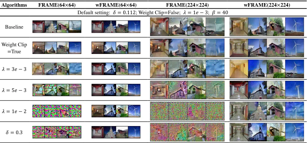
To manifest the superiority of our method over FRAME compared with the baseline settings, we conduct the valida-tion experiments on a subset of SUN dataset (Xiao et al. 2010) under different circumstances. Intuitively, a simple trick to the model collapse issue is to restrict θ in a safe range, a.k.a. weight clipping. The experimental settings in-clude respectively alteringλandδto an insecure range, turn-ing on or off the weight clippturn-ing and varyturn-ing the inputs di-mensions. The results are presented in Fig. 3, which shows the property of a more robust generation compared with the original strategy or FRAME with weight clipping trick.
Empirical Setup on Common Datasets
We apply wFRAME on several widely used datasets in the field of generative modeling. As for default experimental settings, σ = 0.01,β = 60, the number of learning itera-tions is set toT = 100, the step numberLof Langevin sam-pling within each learning iteration is50and the batch size is
N =M = 9. The implementation ofΦ(x)in our method is the first 4 convolutional layers of a pre-learned VGG-16 (Si-monyan and Zisserman 2014). Input shape varies by datasets and is specified following. The hyper-parameters appear in Algorithm 1 differs on each dataset in order to achieve the best results. As for FRAME we use default settings in (Lu, Zhu, and Wu 2015).
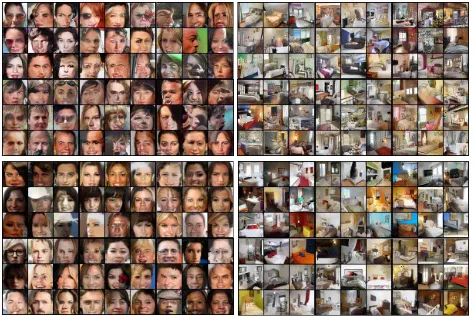
CelebA(Liu et al. 2015) andLSUN-Bedroom(Yu et al. 2015) images are cropped and resized to 64×64. we set
λ= 1e−3in both datasets,δ= 0.2in CelebA andδ= 0.15
in LSUN-Bedroom. The visualizations of two methods are exhibited in Fig. 2.
CIFAR-10(Krizhevsky and Hinton 2009) includes var-ious categories and we learn both algorithms conditioned
Algorithms FRAME(64×64) wFRAME(64×64) FRAME(224×224) wFRAME(224×224)
Default setting: 𝛿𝛿= 0.112; Weight Clip=False; 𝜆𝜆= 1𝑒𝑒 −3; 𝛽𝛽= 40
Baseline
Weight Clip
=True
𝜆𝜆= 3𝑒𝑒 −3
𝜆𝜆= 5𝑒𝑒 −3
𝜆𝜆= 1𝑒𝑒 −2
𝛿𝛿= 0.3
Figure 3: The synthesized results under different circumstances.
on the class label. In this experiment, we set δ = 0.15,
λ = 2e−3 and images’ size are of 32×32. Numerically
and visually in Fig. 4, 5 and Table 1, the results show great improvement.
For a fair comparison, two metrics are utilized to evaluate FRAME and wFRAME. We offer a new metric response dis-tance to measure the disparity between two distributions ac-cording to the results sampled out, while the Inception score is a widely used standard in measuring samples diversity.
Response distanceRis defined as
R= 1
K
K
X
k=1
1
N
N
X
i=1
Fk(xi)− 1
M
M
X
i=1
Fk(yi)
where Fk denotes the kth filter. The smaller the R is, the better the generated results will be, since R ∝
maxθEr[F(yi)]−EPθ[F(x
i)], which implies thatR pro-vides an approximation of the divergence between the target data distribution and the generated data distribution. Further-more, by Eq. 2, the fasterRfalls the betterθconverges.
0 50 100 iters 0
200 400 600 800 1000
response distance
LSUN-Bedroom algorithm FRAME wFRAME
0 50 100 iters CIFAR-10
algorithm FRAME wFRAME
0 50 100 iters CelebA
algorithm FRAME wFRAME
Figure 4: The averaged learning curves of response distance
Ron CelebA, LSUN-Bedroom and CIFAR-10.
Inception score (IS)is the most widely adopted metric of generative models, which estimates the diversity of the
gen-erated samples. It uses a network Inception v2 (Szegedy et al. 2016) pre-trained on ImageNet (Deng et al. 2009) to cap-ture the classifiable properties of samples. This method has the drawbacks of neglecting the visual quality of the gener-ated results and prefers models who generate objects rather than realistic scene images, but it can still provide essential diversity information of synthesized samples in evaluating generative models.
Model Type Name Inception Score
Real Images 11.24±0.11
Implicit Models
DCGAN 6.16±0.07
Improved GAN 4.36±0.05 ALI 5.34±0.05
Descriptive Models
WINN-5CNNs 5.58±0.05 FRAME (wl) 4.95±0.05 FRAME 4.28±0.05 wFRAME (ours,wl) 6.05±0.13
wFRAME (ours) 5.52±0.13
Table 1: Inception score on datasets CIFAR-10 where ’wl’ means training with labels. The IS result of ALI is reported in (Warde-Farley and Bengio 2016). IS of DCGAN is re-ported in (Wang and Liu 2016), and the result of Improved GAN(wl) is reported in (Salimans et al. 2016). WINN’s is reported in (Lee et al. 2018). In the Descriptive Model plate, wFRAME outperforms the most methods.
Comparison with GANs
wFRAME FRAME
plane car bird cat deer dog frog horse ship truck
Figure 5: Images generated by two algorithms conditioned on labels in CIFAR-10, every three columns are of one class, the first group is from FRAME and the second is from wFRAME.
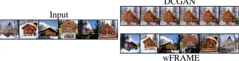
implicit model. GANs with high scores perform badly in descriptive situations, for example, the image reconstruction task or training on a small amount of data. FRAME can han-dle most of these situations properly. The performance of DCGAN in modeling mere few images is presented in Fig. 6 where for equal comparison, we duplicate the input images several times to the total amount of 10000 to adopt the train-ing environment of DCGAN. The compared wFRAME is trained in our own method. The DCGAN’s training proce-dure is ceased as it converges but still remains collapsed re-sults.
Input
DCGAN
wFRAME
Figure 6: The first left row is the selected input images from the SUN dataset, the right first row is the random outputs of DCGAN, the right last row is the outputs of our method.
Comparison of FRAME and wFRAME
From two aspects, we analyze FRAME and wFRAME as a summary of the whole experiments conducted above. As ex-pected, our algorithm is more suitable for synthesizing com-plex and varied scene images and the resulting images are apparently more authentic compared with FRAME.
Quality of Generation Improvement. According to our performances on response distance R, the quality of the image synthesis is improved. This measurement is corre-sponding with the iteration learning process of both FRAME and wFRAME. The learning curves presented in Fig. 4 are the observations of the overall datasets synthesis. From the curves can we draw the conclusion that wFRAME converges better than FRAME. The results of generation on CelebA, LSUN-Bedroom and CIFAR-10 in Fig. 2 and 5 shows that even if the training images are relatively aligned with
con-spicuous structural information, or with only simple categor-ical context information, the images produced by FRAME are still abundant with motley noise and twisted texture, while ours are more reasonably mixed, more sensible struc-tured and bright-colored with less distortion.
Training Steadiness Improvement. Compared with FRAME as shown in Fig. 1 which illustrates the typical evolution of generated samples, we found an improvement in the training steadiness. The generated images are almost identical at the beginning, however, images produced by our algorithm are able to be back on track after 30 iterations while FRAME’s deteriorate. Quantitatively in Fig. 4, the curves are calculated by averaging across the whole dataset. wFRAME reaches lower cost on response distance, namely the direct L1 critic of filter banks between synthesized
samples and target samples is smaller and decreases more steadily. To be more specific, our algorithm has mostly solved the model collapse problem of FRAME for it not only ensures the closeness between the generated samples and “ground-truth” samples but also stabilizes the learning phase of the model parameter θ. The three plots clearly show the quantitative measures are well correlated with qualitative visualizations of generated samples. In the absence of collapsing, we attain comparable or even better results over FRAME.
Conclusion
promising results.
References
Adams, S.; Dirr, N.; Peletier, M. A.; and Zimmer, J. 2011. From a large-deviations principle to the wasserstein gradi-ent flow: a new micro-macro passage. Communications in Mathematical Physics307(3):791–815.
Ambrosio, L.; Gigli, N.; and Savar´e, G. 2008. Gradient flows: in metric spaces and in the space of probability mea-sures. Springer Science & Business Media.
Arjovsky, M.; Chintala, S.; and Bottou, L. 2017. Wasser-stein generative adversarial networks. InInternational Con-ference on Machine Learning, 214–223.
Benamou, J.-D., and Brenier, Y. 2000. A computational fluid mechanics solution to the monge-kantorovich mass transfer problem.Numerische Mathematik84(3):375–393.
Dai, J.; Lu, Y.; and Wu, Y.-N. 2014. Generative mod-eling of convolutional neural networks. arXiv preprint arXiv:1412.6296.
Deng, J.; Dong, W.; Socher, R.; Li, L.-J.; Li, K.; and Fei-Fei, L. 2009. Imagenet: A large-scale hierarchical im-age database. InComputer Vision and Pattern Recognition (CVPR), 2009. IEEE Conference on, 248–255. IEEE.
Duong, M. H.; Laschos, V.; and Renger, M. 2013. Wasser-stein gradient flows from large deviations of many-particle limits.ESAIM: Control, Optimisation and Calculus of Vari-ations19(4):1166–1188.
Erbar, Matthias anErbar, M.; Maas, J.; Renger, M.; et al. 2015. From large deviations to wasserstein gradient flows in multiple dimensions. Electronic Communications in Proba-bility20.
Goodfellow, I.; Pouget-Abadie, J.; Mirza, M.; Xu, B.; Warde-Farley, D.; Ozair, S.; Courville, A.; and Bengio, Y. 2014. Generative adversarial nets. InAdvances in Neural Information Processing Systems, 2672–2680.
Jordan, R.; Kinderlehrer, D.; and Otto, F. 1998. The vari-ational formulation of the fokker–planck equation. SIAM journal on mathematical analysis29(1):1–17.
Koller, D., and Friedman, N. 2009. Probabilistic graphical models: principles and techniques. MIT press.
Krizhevsky, A., and Hinton, G. 2009. Learning multiple lay-ers of features from tiny images. Technical report, Citeseer. Krizhevsky, A.; Sutskever, I.; and Hinton, G. E. 2012. Imagenet classification with deep convolutional neural net-works. InAdvances in neural information processing sys-tems, 1097–1105.
Landau, L. D., and Lifshitz, E. M. 2013. Course of theoret-ical physics. Elsevier.
Lee, K.; Xu, W.; Fan, F.; and Tu, Z. 2018. Wasserstein introspective neural networks. InThe IEEE Conference on Computer Vision and Pattern Recognition (CVPR).
Liu, Z.; Luo, P.; Wang, X.; and Tang, X. 2015. Deep learn-ing face attributes in the wild. InProceedings of the IEEE International Conference on Computer Vision, 3730–3738.
Lu, Y.; Zhu, S.-C.; and Wu, Y. N. 2015. Learning frame models using cnn filters. arXiv preprint arXiv:1509.08379. Montavon, G.; M¨uller, K.-R.; and Cuturi, M. 2016. Wasser-stein training of restricted boltzmann machines. InAdvances in Neural Information Processing Systems, 3718–3726. Rubner, Y.; Tomasi, C.; and Guibas, L. J. 2000. The earth mover’s distance as a metric for image retrieval. Interna-tional journal of computer vision40(2):99–121.
Salimans, T.; Goodfellow, I.; Zaremba, W.; Cheung, V.; Rad-ford, A.; and Chen, X. 2016. Improved techniques for train-ing gans. In Advances in Neural Information Processing Systems, 2234–2242.
Simonyan, K., and Zisserman, A. 2014. Very deep convo-lutional networks for large-scale image recognition. arXiv preprint arXiv:1409.1556.
Szegedy, C.; Vanhoucke, V.; Ioffe, S.; Shlens, J.; and Wojna, Z. 2016. Rethinking the inception architecture for computer vision. InProceedings of the IEEE conference on computer vision and pattern recognition, 2818–2826.
Villani, C. 2003. Topics in optimal transportation. Num-ber 58. American Mathematical Soc.
Wang, D., and Liu, Q. 2016. Learning to draw samples: With application to amortized mle for generative adversarial learning.arXiv preprint arXiv:1611.01722.
Warde-Farley, D., and Bengio, Y. 2016. Improving genera-tive adversarial networks with denoising feature matching. Xiao, J.; Hays, J.; Ehinger, K. A.; Oliva, A.; and Torralba, A. 2010. Sun database: Large-scale scene recognition from abbey to zoo. InComputer vision and pattern recognition (CVPR), 2010 IEEE conference on, 3485–3492. IEEE. Xie, J.; Lu, Y.; Zhu, S.-C.; and Wu, Y. N. 2016a. Cooperative training of descriptor and generator networks.arXiv preprint arXiv:1609.09408.
Xie, J.; Lu, Y.; Zhu, S.-C.; and Wu, Y. 2016b. A theory of generative convnet. InInternational Conference on Machine Learning, 2635–2644.
Xie, J.; Zheng, Z.; Gao, R.; Wang, W.; Zhu, S.-C.; and Wu, Y. N. 2018. Learning descriptor networks for 3d shape syn-thesis and analysis. arXiv preprint arXiv:1804.00586. Xie, J.; Zhu, S.-C.; and Wu, Y. N. 2017. Synthesizing dy-namic patterns by spatial-temporal generative convnet. In Proceedings of the IEEE Conference on Computer Vision and Pattern Recognition, 7093–7101.
Younes, L. 1989. Parametric inference for imperfectly observed gibbsian fields. Probability Theory and Related Fields82(4):625–645.
Yu, F.; Zhang, Y.; Song, S.; Seff, A.; and Xiao, J. 2015. Lsun: Construction of a large-scale image dataset using deep learning with humans in the loop. arXiv preprint arXiv:1506.03365.