On solving the split generalized equilibrium problem and the fixed point problem for a countable family of nonexpansive multivalued mappings

(1)

R E S E A R C H

Open Access

On solving the split generalized

equilibrium problem and the ﬁxed point

problem for a countable family of

nonexpansive multivalued mappings

Withun Phuengrattana

1,2*

_{and Kritsada Lerkchaiyaphum}

1

*_{Correspondence:}

[email protected]

1_{Department of Mathematics,}

Faculty of Science and Technology, Nakhon Pathom Rajabhat University, Nakhon Pathom, Thailand

2_{Research Center for Pure and}

Applied Mathematics, Research and Development Institute, Nakhon Pathom Rajabhat University, Nakhon Pathom, Thailand

Abstract

We consider the split generalized equilibrium problem and the ﬁxed point problem for a countable family of nonexpansive multivalued mappings in real Hilbert spaces. Then, using the shrinking projection method, we prove a strong convergence theorem for ﬁnding a common solution of the considered problems. A numerical example is presented to illustrate the convergence result. Our results improve and extend the corresponding results in the literature.

MSC: 47H09; 47H10; 65K10; 65K15

Keywords: Fixed point problems; Split generalized equilibrium problems; Nonexpansive multivalued mapping; Hilbert spaces

1 Introduction

LetHbe a real Hilbert space with inner product·,·and induced norm · . LetCbe a nonempty closed convex subset ofH, ϕ:C×C→R, and letF:C×C→Rbe two bifunctions. Thegeneralized equilibrium problemis to ﬁndx∈Csuch that

F(x,y) +ϕ(x,y)≥0, ∀y∈C. (1.1)

The solution set of generalized equilibrium problem is denoted byGEP(F,ϕ). In particular, ifϕ= 0, then this problem reduces to the equilibrium problem to ﬁndx∈C such that F(x,y)≥0 for ally∈C. The solution set of the equilibrium problem is denoted byEP(F). The generalized equilibrium problem is very general in the sense that it includes, as particular cases, optimization problems, variational inequality problems, minimization problems, ﬁxed point problems, mixed equilibrium problem, Nash equilibrium problems in noncooperative games, and others; see, for example, [1–6].

In 2013, Kazmi and Rizvi [7] introduced and studied the following split generalized equi-librium problem. LetC⊆H1andQ⊆H2, letF1,ϕ1:C×C→RandF2,ϕ2:Q×Q→R be nonlinear bifunctions, and letA:H1→H2 be a bounded linear operator. Thesplit

(2)

generalized equilibrium problemis to ﬁndx∗∈Csuch that

F1x∗,x+ϕ1

x∗,x≥0, ∀x∈C, (1.2)

and such that

y∗=Ax∗∈Q solves F2y∗,y+ϕ2

y∗,y≥0, ∀y∈Q. (1.3)

The solution set of the split generalized equilibrium problem is denoted by

SGEP(F1,ϕ1,F2,ϕ2) :=x∗∈C:x∗∈GEP(F1,ϕ1) andAx∗∈GEP(F2,ϕ2).

The authors also gave an iterative algorithm to ﬁnd a common element of the solution sets of the split generalized equilibrium problem in real Hilbert spaces; for more details, we refer to [7–9]. If ϕ1= 0 andϕ2= 0, then the split generalized equilibrium problem reduces to the split equilibrium problem; see [10]. IfF2= 0 andϕ2= 0, the split generalized equilibrium problem reduces to the equilibrium problem considered by Cianciaruso et al. [11].

In 2008, Takahashi et al. [12] introduced the following iterative algorithm, which is known as the shrinking projection method, for finding a fixed point of a nonexpansive single-valued mapping in Hilbert spaces. The shrinking projection method is a popu-lar method and plays an important role in studying the strong convergence for finding fixed points of nonlinear mappings. Many researchers developed the shrinking projection method for solving variational inequality problems, equilibrium problems, and fixed point problems in Hilbert spaces; see, for example, [13, 14].

Motivated and inspired by the results mentioned and related literature, we propose an it-erative algorithm based on the shrinking projection method for ﬁnding a common element of the set of solutions of split generalized equilibrium problems and the set of common ﬁxed points of a countable family of nonexpansive multivalued mappings in real Hilbert spaces. Then we prove strong convergence theorems that extend and improve the corre-sponding results of Kazmi and Rizvi [7], Suantai et al. [15], and others. Finally, we give some examples and numerical results to illustrate our main results.

2 Preliminaries

LetCbe a nonempty closed convex subset of a real Hilbert spaceH. We denote the strong convergence and the weak convergence of a sequence{xn} to a pointx∈H byxn→x andxnx, respectively. It is also well known [16] that a Hilbert spaceHsatisﬁesOpial’s condition, that is, for any sequence{xn}withxnx, the inequality

lim sup

n→∞

xn–x<lim sup n→∞

xn–y

holds for everyy∈Hwithy=x.

The following three lemmas are useful for our main results.

(3)

(2) x+y2_{≤ x}2_{+ 2y,}_x₊_y,_∀x,_y_∈_H;

(3) If{xn}is a sequence inHthat converges weakly toz∈H,then

lim sup

n→∞ xn–y

2₌_{lim sup}

n→∞ xn–z

2₊_z_–_y2_, _∀_y_∈_H.

Lemma 2.2([17]) Let H be a Hilbert space.Let x1,x2, . . . ,xN∈H,and letα1,α2, . . . ,αNbe real numbers such thatN_i₌₁αi= 1.Then

N

i=1

αixi 2

= N

i=1

αixi2–

1≤i,j≤N

αiαjxi–xj2.

Lemma 2.3([18]) Let H be a Hilbert space,and let{xn}be a sequence in H.Let u,v∈H be such thatlim_n_→∞xn–uandlimn→∞xn–vexist.If{xnk}and{xmk}are subsequences

of{xn}that converge weakly to u and v,respectively,then u=v.

A single-valued mappingT:C→His calledδ-inverse strongly monotone[19] if there exists a positive real numberδsuch that

x–y,Tx–Ty ≥δTx–Ty2, ∀x,y∈C.

For eachγ ∈(0, 2δ], we see thatI–γT is a nonexpansive single-valued mapping, that is,

(I–γT)x– (I–γT)y≤ x–y, ∀x,y∈C.

We denote byCB(C) andK(C) the collections of all nonempty closed bounded subsets and nonempty compact subsets ofC, respectively. TheHausdorﬀ metricHonCB(C) is deﬁned by

H(A,B) :=max sup

x∈A

dist(x,B),sup

y∈B

dist(y,A)

, ∀A,B∈CB(C),

wheredist(x,B) =inf{d(x,y) :y∈B}is the distance from a pointxto a subsetB. LetS:C→ CB(C) be a multivalued mapping. An elementx∈Cis called aﬁxed pointofSifx∈Sx. The set of all ﬁxed points ofSis denoted byF(S), that is,F(S) ={x∈C:x∈Sx}. Recall that a multivalued mappingS:C→CB(C) is called

(i) nonexpansiveif

H(Sx,Sy)≤ x–y, ∀x,y∈C;

(ii) quasi-nonexpansiveifF(S)=∅and

H(Sx,Sp)≤ x–p, ∀x∈C,∀p∈F(S).

(4)

Lemma 2.4 ([21]) Let C be a nonempty closed convex subset of a real Hilbert space H. Let S:C→CB(C)be a nonexpansive multivalued mapping with F(S)=∅and Sp={p}for each p∈F(S).Then F(S)is a closed and convex subset of C.

Lemma 2.5 ([22]) Let C be a nonempty closed convex subset of a real Hilbert space H. Given x,y,z∈H and a real numberα,the set{u∈C:y–u2≤ x–u2+z,u+α}is closed and convex.

Lemma 2.6([23, 24]) Let C be a nonempty closed convex subset of a real Hilbert space H, and let PC:H→C be the metric projection.Then

y–PCx2+x–PCx2≤ x–y2, ∀x∈H,y∈C.

For solving the generalized equilibrium problem, we assume that the bifunctionsF1: C×C→Randϕ1:C×C→Rsatisfy the following assumption.

Assumption 2.7 LetCbe nonempty closed and convex subset of a Hilbert spaceH1. Let F1:C×C→Randϕ1:C×C→Rbe two bifunctions satisfy the following conditions:

(A1) F1(x,x) = 0for allx∈C,

(A2) F1is monotone, that is,F1(x,y) +F1(y,x)≤0for allx,y∈C, (A3) F1is upper hemicontinuous,that is, for allx,y,z∈C,

limt↓0F1(tz+ (1 –t)x,y)≤F1(x,y),

(A4) for eachx∈C,y→F1(x,y)is convex and lower semicontinuous, (A5) ϕ1(x,x)≥0for allx∈C,

(A6) for eachy∈C,x→ϕ1(x,y)is upper semicontinuous,

(A7) for eachx∈C,y→ϕ1(x,y)is convex and lower semicontinuous,

and assume that for ﬁxedr> 0 andz∈C, there exists a nonempty compact convex subset KofH1andx∈C∩Ksuch that

F1(y,x) +ϕ1(y,x) +1

ry–x,x–z< 0, ∀y∈C\K.

Lemma 2.8([25]) Let C be nonempty closed and convex subset of a Hilbert space H1.Let F1:C×C→Randϕ1:C×C→Rbe two bifunctions satisfy Assumption2.7.Assume thatϕ1is monotone.For r> 0and x∈H1,deﬁne a mapping T(F1,

ϕ1)

r :H1→C as follows:

T_r(F1,ϕ1)(x) =

z∈C:F1(z,y) +ϕ1(z,y) +1

ry–z,z–x ≥0,∀y∈C

for all x∈H1.Then:

(1) For eachx∈H1,Tr(F1,ϕ1)=∅, (2) Tr(F1,ϕ1)is single-valued,

(3) Tr(F1,ϕ1)is ﬁrmly nonexpansive,that is,for anyx,y∈H1,

T(F1,ϕ1)

r x–Tr(F1,ϕ1)y 2

≤T(F1,ϕ1)

r x–Tr(F1,ϕ1)y,x–y

,

(4) F(Tr(F1,ϕ1)) =GEP(F1,ϕ1),

(5)

Further,assume that F2:Q×Q→Randϕ2:Q×Q→Rsatisfy Assumption2.7,where Q is a nonempty closed and convex subset of a Hilbert space H2.For all s> 0and w∈H2, deﬁne the mapping T(F2,ϕ2)

s :H2→Q by

T_s(F2,ϕ2)(v) =

w∈Q:F2(w,d) +ϕ2(w,d) +1

rd–w,w–v ≥0,∀d∈Q

.

Then we have:

(6) For eachv∈H2,Ts(F2,ϕ2)=∅, (7) Ts(F2,ϕ2)is single-valued, (8) Ts(F2,ϕ2)is ﬁrmly nonexpansive, (9) F(Ts(F2,ϕ2)) =GEP(F2,ϕ2), (10) GEP(F2,ϕ2)is closed and convex,

whereGEP(F2,ϕ2)is the solution set of the following generalized equilibrium problem:

Findy∗∈Qsuch thatF2(y∗,y) +ϕ2(y∗,y)≥0for ally∈Q.

Moreover,SGEP(F1,ϕ1,F2,ϕ2)is a closed and convex set.

Lemma 2.9([11]) Let C be nonempty closed and convex subset of a Hilbert space H1.Let F1:C×C→Randϕ1:C×C→Rbe two bifunctions satisfying Assumption2.7,and let Tr(F1,ϕ1)be deﬁned as in Lemma2.8for r> 0.Let x,y∈H1and r1,r2> 0.Then

T(F1,ϕ1) r2 y–T

(F1,ϕ1)

r1 x≤ y–x+

r2_r2–r1T(F1,ϕ1) r2 y–y.

3 Main results

In this section, we prove strong convergence theorems for ﬁnding a common element of the set of solutions of split generalized equilibrium problems and the set of common ﬁxed points of a countable family of nonexpansive multivalued mappings in real Hilbert spaces and give a numerical example to support our main result.

We now state and prove our main result.

Theorem 3.1 Let C be a nonempty closed convex subset of a real Hilbert space H1,and let Q be a nonempty closed convex subset of a real Hilbert space H2.Let A:H1 →H2 be a bounded linear operator,and let {Si} be a countable family of nonexpansive mul-tivalued mappings of C into CB(C).Let F1,ϕ1:C×C→R, F2,ϕ2:Q×Q→Rbe bi-functions satisfying Assumption 2.7. Let ϕ1, ϕ2 be monotone, ϕ1 be upper hemicontin-uous, and F2 andϕ2 be upper semicontinuous in the ﬁrst argument. Assume that = ∞

i=1F(Si)∩SGEP(F1,ϕ1,F2,ϕ2)=∅and Sip={p}for each p∈ ∞

i=1F(Si).Let x1∈C with C1=C,and let{xn}be a sequence generated by

⎧ ⎪ ⎪ ⎪ ⎪ ⎪ ⎨ ⎪ ⎪ ⎪ ⎪ ⎪ ⎩

un=Tr(nF1,ϕ1)(I–γA∗(I–T

(F2,ϕ2) rn )A)xn,

zn=α(0)n xn+αn(1)y(1)n +· · ·+αn(n)y(nn), yn(i)∈Siun,

Cn+1={p∈Cn:zn–p ≤ xn–p},

xn+1=PCn+1x1, n∈N,

(3.1)

where{αn(i)} ⊂(0, 1)satisfy n

i=0α (i)

(6)

(C1) The limitslimn→∞αn(i)∈(0, 1)exist for alli≥0, (C2) lim infn→∞rn> 0.

Then the sequence{xn}generated by(3.1)converges strongly to Px1.

Proof We divide our proof into six steps.

Step1. We show that{xn}is well-deﬁned for everyn∈N.

By Lemmas 2.4 and 2.8 we obtain thatSGEP(F1,ϕ1,F2,ϕ2) and∞_i₌₁F(Si) are closed and convex subsets ofC. Henceis a closed and convex subset ofC. It follows by Lemma 2.5 thatCn+1is closed and convex for eachn∈N.

Letp∈. Then we havep=T(F1,ϕ1)

rn pandAp=T

(F2,ϕ2)

rn (Ap). It follows thatp= (I–γA∗(I–

Tr(Fn2,ϕ2))A)p. SinceT

(F1,ϕ1) rn andT

(F2,ϕ2)

rn both are ﬁrmly nonexpansive, forγ ∈(0,1_L), the

mappingT(F1,ϕ1)

rn (I–γA∗(I–T

(F2,ϕ2)

rn )A) is nonexpansive; see [26]. This implies that

un–p=Tr(Fn1,ϕ1)

I–γA∗I–T_r(_nF2,ϕ2)Axn–Tr(nF1,ϕ1)

I–γA∗I–T_r(_nF2,ϕ2)Ap

≤ xn–p. (3.2)

Then, sinceSip={p}for allp∈ ∞

i=1F(Si), we have

zn–p ≤αn(0)xn–p+αn(1)y(1)n –p+· · ·+αn(n)y(nn)–p

=α(0)_n xn–p+αn(1)dist

y_n(1),S1p+· · ·+α_n(n)disty(_nn),Snp

≤α_n(0)xn–p+αn(1)H(S1un,S1p) +· · ·+αn(n)H(Snun,Snp)

≤α_n(0)xn–p+αn(1)un–p+· · ·+αn(n)un–p. (3.3)

This implies by (3.2) andn_i₌₀α(ni)= 1 that

zn–p ≤ xn–p. (3.4)

This shows thatp∈Cn+1and hence⊂Cn+1⊂Cn. Therefore,PCn+1x1is well-deﬁned for everyx1∈C. Hence,{xn}is well-deﬁned.

Step2. We show thatlimn→∞xn=qfor someq∈C.

Sinceis a nonempty closed convex subset ofH1, there exists a uniqueω∈such that

ω=Px1. Sincexn=PCnx1andxn+1∈Cn+1⊂Cnfor alln∈N, we havexn–x1 ≤ xn+1–

x1for alln∈N. On the other hand, since⊂Cn, we obtain thatxn–x1 ≤ ω–x1for alln∈N. Hence{xn–x1}is bounded; so are{zn}and{y(ni)}. Therefore,limn→∞xn–x1 exists. By the construction of the setCnwe know thatxm=PCmx1∈Cm⊂Cnform>n≥1. This implies by Lemma 2.6 that

xm–xn2≤ xm–x12–xn–x12→0 asm,n→ ∞. (3.5)

Sincelim_n_→∞xn–x1exists, it follows that{xn}is a Cauchy sequence. By the complete-ness ofH1and the closedness ofCwe get that there exists an elementq∈Csuch that

limn→∞xn=q.

Step3. We show thatlimn→∞yn(i)–xn= 0 for alli∈N. From (3.5) we have

lim

(7)

Sincexn+1∈Cn+1, we get that

zn–xn ≤ zn–xn+1+xn+1–xn ≤ xn–xn+1+xn+1–xn ≤2xn+1–xn.

This implies by (3.6) that

lim

n→∞zn–xn= 0. (3.7)

Thuslim_n_→∞zn=q.

Forp∈, by Lemma 2.2 we see that

zn–p2≤αn(0)xn–p2+ n

i=1

α_n(i)y(_ni)–p2– n

i=1

α_n(0)α(_ni)y(_ni)–xn2

=α(0)_n xn–p2+ n

i=1

α(_ni)disty(_ni),S1p2– n

i=1

α_n(0)α(_ni)y(_ni)–xn 2

=α(0)_n xn–p2+ n

i=1

α(_ni)H(Siun,Sip)2– n

i=1

α_n(0)α(_ni)y(_ni)–xn 2

≤α_n(0)xn–p2+ n

i=1

α_n(i)un–p2– n

i=1

α_n(0)α_n(i)y(_ni)–xn 2

. (3.8)

This implies by (3.2) andn_i₌₀α(ni)= 1 that

zn–p2≤ xn–p2– n

i=1

α(0)_n α_n(i)y(_ni)–xn 2

.

Therefore we have

α(0)_n α_n(i)y(_ni)–xn 2

≤ n

i=1

α(0)_n α_n(i)y(_ni)–xn 2

≤ xn–p2–zn–p2 ≤ xn–zn

xn–p+zn–p

.

By the given control condition on{α(ni)}and (3.7) we obtain

lim

n→∞y

(i)

n –xn= 0, ∀i∈N. (3.9)

Step4. We show thatlimn→∞un–xn= 0. Forp∈, we get that

un–p2=Tr(nF1,ϕ1)

I–γA∗I–T(F2,ϕ2) rn

Axn–Tr(Fn1,ϕ1)p

2

≤I–γA∗I–T(F2,ϕ2) rn

Axn–p 2

≤ xn–p2+γ2A∗

I–T(F2,ϕ2) rn

Axn

2

+ 2γp–xn,A∗

I–T_r(_nF2,ϕ2)Axn

≤ xn–p2+γ2

Axn–Tr(nF2,ϕ2)Axn,AA

∗_I_–_T(F2,ϕ2) rn

Axn

(8)

+ 2γA(p–xn),Axn–Tr(nF2,ϕ2)Axn

≤ xn–p2+Lγ2

Axn–Tr(nF2,ϕ2)Axn,Axn–T

F2 rnAxn

+ 2γA(p–xn) +

Axn–Tr(nF2,ϕ2)Axn

–Axn–TrFn2Axn

,

Axn–Tr(nF2,ϕ2)Axn

≤ xn–p2+Lγ2Axn–Tr(nF2,ϕ2)Axn

2

+ 2γAp–T(F2,ϕ2)

rn Axn,Axn–T

(F2,ϕ2) rn Axn

–Axn–Tr(nF2,ϕ2)Axn

2

≤ xn–p2+Lγ2Axn–Tr(nF2,ϕ2)Axn

2

+ 2γ

1

2Axn–T (F2,ϕ2) rn Axn

2

–Axn–Tr(Fn2,ϕ2)Axn

2

=xn–p2+γ(Lγ– 1)Axn–Tr(nF2,ϕ2)Axn

2 .

Thus by (3.8) we have

i=1

α_n(i)un–p2

≤α_n(0)xn–p+ n

i=1

α_n(i)xn–p2+γ(Lγ – 1)Axn–Tr(Fn2,ϕ2)Axn

2

=xn–p2+γ(Lγ – 1) n

i=1

α_n(i)Axn–Tr(nF2,ϕ2)Axn

2

=xn–p2–γ(1 –Lγ)

1 –α_n(0)Axn–Tr(nF2,ϕ2)Axn

2

. (3.10)

Therefore we have

γ(1 –Lγ)1 –α_n(0)Axn–Tr(Fn2,ϕ2)Axn

2

≤ xn–p2–zn–p2 ≤ xn–zn

xn–p+zn–p

.

By the given control condition on{α(0)n },γ(1 –Lγ) > 0, and (3.7) we obtain that

lim

n→∞Axn–T (F2,ϕ2)

rn Axn= 0. (3.11)

SinceT(F1,ϕ1)

rn is ﬁrmly nonexpansive andI–γA∗(I–T

(F2,ϕ2)

rn )Ais nonexpansive, we have

un–p2=Tr(nF1,ϕ1)

Axn–Tr(Fn1,ϕ1)p

2

≤T(F1,ϕ1) rn

I–γA∗I–T_r(_nF2,ϕ2)Axn–TrFn1p,

Axn–p

=un–p,

Axn–p

= 1 2

un–p2+I–γA∗

I–T_r(_nF2,ϕ2)Axn–p 2

–un–xn–γA∗

(9)

≤ 1 2

un–p2+xn–p2–

un–xn2+γ2A∗

I–T(F2,ϕ2) rn

Axn

2

– 2γun–xn,A∗

I–T_r(F_n2,ϕ2)Axn

,

which implies that

un–p2≤ xn–p2–un–xn2+ 2γ

un–xn,A∗

I–T(F2,ϕ2) rn

Axn

≤ xn–p2–un–xn2+ 2γun–xnA∗

I–T(F2,ϕ2) rn

Axn. (3.12)

This implies by (3.8) that

i=1

α_n(i)un–p2

≤α_n(0)xn–p+ n

i=1

α_n(i)xn–p2–un–xn2

+ 2γun–xnA∗

I–T(F2,ϕ2) rn

Axn

=xn–p2–

1 –α(0)_n un–xn2

+ 2γ1 –α_n(0)un–xnA∗

I–T_r(_nF2,ϕ2)Axn

=xn–p2–

1 –α(0)_n un–xn2

+ 2γ1 –α_n(0)un–xnA∗

I–T(F2,ϕ2) rn

Axn.

Therefore we have

1 –α_n(0)un–xn2

≤ xn–p2–zn–p2+ 2γ

1 –α(0)_n un–xnA∗

I–T(F2,ϕ2) rn

Axn

≤ xn–p2–zn–p2+ 2γ

1 –α(0)_n MA∗I–T(F2,ϕ2) rn

Axn ≤ xn–zn

xn–p+zn–p

+ 2γ1 –α(0)_n MA∗I–T_r(_nF2,ϕ2)Axn,

whereM=sup{un–xn:n∈N}. This implies by Condition (C1), (3.7), and (3.11) that

lim

n→∞un–xn= 0. (3.13)

Step5. We show thatq∈∞_i₌₁F(Si). By (3.9) and (3.13), for alli∈N, we get that

lim

n→∞dist(un,Siun)≤nlim→∞un–y (i) n ≤ lim

n→∞un–xn+nlim→∞xn–y

(i) n

(10)

For eachi∈N, we get

dist(q,Siq)≤ q–un+un–y(ni)+dist

y(_ni),Siq

≤ q–un+dist(un,Siun) +H(Siun,Siq) ≤2q–un+dist(un,Siun)

≤2q–zn+zn–xn

+dist(un,Siun).

Sincelimn→∞zn=q, it follows by (3.7) and (3.14) that

dist(q,Siq) = 0 for alli∈N.

This shows thatq∈Siqfor alli∈N, and henceq∈ ∞

i=1F(Si). Step6. We show thatq∈SGEP(F1,ϕ1,F2,ϕ2).

First, we will show thatq∈GEP(F1,ϕ1). Sinceun=Tr(nF1,ϕ1)(I–γA∗(I–T

(F2,ϕ2)

rn )A)xn, we have

F1(un,y) +ϕ1(un,y) + 1 rn

y–un,un–xn–γA∗

I–T_r(_nF2,ϕ2)Axn

≥0, ∀y∈C,

which implies that

F1(un,y) +ϕ1(un,y) + 1 rny–

un,un–xn– 1 rn

y–un,γA∗

I–T_r(F_n2,ϕ2)Axn

≥0, ∀y∈C.

It follows from the monotonicity ofF1andϕ1that

1 rn

y–un,un–xn– 1 rn

y–un,γA∗

I–T(F2,ϕ2) rn

Axn

≥F1(y,un) +ϕ1(y,un), ∀y∈C.

By (3.13) andlim_n_→∞xn=qwe get thatlimn→∞un=q. It follows by Condition (C2), (3.11), (3.13), Assumption 2.7, (A4) and (A7), that 0≥F1(y,q) +ϕ1(y,q) for all y∈C. Putyt= ty+ (1 –t)qfor allt∈(0, 1] andy∈C. Consequently, we getyt∈C, and henceF1(yt,q) +

ϕ1(yt,q)≤0. So by Assumption 2.7, (A1)–(A7), we have

0≤F1(yt,yt) +ϕ1(yt,yt)

≤tF1(yt,y) +ϕ1(yt,y)

+ (1 –t)F1(yt,q) +ϕ1(yt,q)

≤tF1(yt,y) +ϕ1(yt,y)

+ (1 –t)F1(q,yt) +ϕ1(q,yt)

≤F1(yt,y) +ϕ1(yt,y).

Hence we have

F1(yt,y) +ϕ1(yt,y)≥0, ∀y∈C.

Lettingt→0, by Assumption 2.7 (A3) and the upper hemicontinuity ofϕ1we have

F1(q,y) +ϕ1(q,y)≥0, ∀y∈C.

(11)

Next, we show thatAq∈GEP(F2,ϕ2).

SinceAis a bounded linear operator, we haveAxn→Aq. Then, it follows from (3.11) that

T(F2,ϕ2)

rn Axn→Aq. (3.15)

By the deﬁnition ofT(F2,ϕ2)

rn Axnwe have

F2T_r(_nF2,ϕ2)Axn,y

+ϕ2

T_r(_nF2,ϕ2)Axn,y

+ 1 rn

y–T_r(_nF2,ϕ2)Axn,Tr(Fn2,ϕ2)Axn–Axn

≥0

for ally∈Q. SinceF2andϕ2are upper semicontinuous in the ﬁrst argument, it follows by (3.15) that

F2(Aq,y) +ϕ2(Aq,y)≥0, ∀y∈Q.

This shows thatAq∈GEP(F2,ϕ2). Thereforeq∈SGEP(F1,ϕ1,F2,ϕ2). By Steps 5 and 6 we get thatq∈.

Step7. Finally, we show thatq=Px1.

Sincexn=PCnx1and⊂Cn, we obtainx1–xn,xn–p ≥0 for allp∈. Thus we get x1–q,q–p ≥0 for allp∈. This shows thatq=Px1.

By Steps 1–7 we can conclude that{xn}converges strongly toPx1. This completes the

proof.

Ifϕ1=ϕ2= 0, then the split generalized equilibrium problem reduces to the split equi-librium problem. So, the following result can be immediately obtained from Theorem 3.1.

Corollary 3.2 Let C be a nonempty closed convex subset of a real Hilbert space H1,and let Q be a nonempty closed convex subset of a real Hilbert space H2.Let A:H1→H2be a bounded linear operator,and let{Si}be a countable family of nonexpansive multivalued mappings of C into CB(C).Let F1:C×C→R,F2:Q×Q→Rbe bifunctions satisfying Assumption2.7.Let F2 be upper semicontinuous in the ﬁrst argument.Assume that= ∞

i=1F(Si)∩SEP(F1,F2)=∅and Sip={p}for each p∈ ∞

i=1F(Si).Let x1∈C with C1=C, and let{xn}be a sequence generated by

⎧ ⎪ ⎪ ⎪ ⎪ ⎪ ⎨ ⎪ ⎪ ⎪ ⎪ ⎪ ⎩

un=TrFn1(I–γA∗(I–T

F2 rn)A)xn,

Cn+1={p∈Cn:zn–p ≤ xn–p},

(3.16)

i=0α (i)

n = 1,{rn} ⊂(0,∞),andγ ∈(0,1_L),where L is the spectral radius of A∗A,and A∗is the adjoint of A.Assume that the following conditions hold:

(C1) The limitslimn→∞αn(i)∈(0, 1)exist for alli≥0, (C2) lim inf_n_→∞rn> 0.

(12)

IfF1=F2=F,H1=H2=H, andϕ1=ϕ2= 0, then the following result can be immediately obtained from Theorem 3.1.

Corollary 3.3 Let C be a nonempty closed convex subset of a real Hilbert space H.Let

A:H→H be a bounded linear operator,and let{Si}be a countable family of nonexpansive multivalued mappings of C into CB(C).Let F:C×C→Rbe a bifunction satisfying As-sumption2.7.Assume that=∞_i₌₁F(Si)∩EP(F)=∅and Sip={p}for each p∈

_∞ i=1F(Si). Let x1∈C with C1=C,and let{xn}be a sequence generated by

⎧ ⎪ ⎪ ⎪ ⎪ ⎪ ⎨ ⎪ ⎪ ⎪ ⎪ ⎪ ⎩

un=TrFn(I–γA

∗_(I_–_TF rn)A)xn,

Cn+1={p∈Cn:zn–p ≤ xn–p},

(3.17)

i=0α (i)

n = 1,{rn} ⊂(0,∞),andγ ∈(0,1_L),where L is the spectral radius of A∗A,and A∗is the adjoint of A.Assume that the following conditions hold:

(C1) The limitslimn→∞αn(i)∈(0, 1)exist for alli≥0, (C2) lim infn→∞rn> 0.

Then the sequence{xn}generated by(3.17)converges strongly to Px1.

4 Numerical example

In this section, we present a numerical example to demonstrate the performance and con-vergence of our theoretical results. All codes were written in Scilab.

Example 4.1 LetH1=H2=RandC=Q= [0, 10]. LetA:H1→H2be deﬁned byAx= x for eachx∈H1. ThenA∗y=yfor eachy∈H2. For x∈C, i= 1, 2, . . . , we deﬁne the multivalued mappingsSionCas follows:

Six=

0, x 10i

for alli∈N.

Obviously,Si is nonexpansive for alli∈N,Si(0) ={0}, and ∞

i=1F(Si) ={0}. Define the bifunctionsF1,ϕ1:C×C→RbyF1(x,y) =y2+ 3xy– 4x2andϕ1(x,y) =y2–x2forx,y∈C. DefineF2,ϕ2:Q×Q→RbyF2(w,v) = 2v2+wv– 3w2andϕ2(w,v) =w–vforw∈Qand v∈Q. Choosern=_nn₊₁,γ =₁₀1, and the sequences{λ(ni)}defined by

λ(_ni)= ⎧ ⎪ ⎪ ⎨ ⎪ ⎪ ⎩

1

bi+1(_nn₊₁), n≥i+ 1, 1 –_nn₊₁(n_k₌₁_b1k), n=i,

0, n<i,

(13)

For allx∈Candn∈N, we computeTr(F2,ϕ2)Ax. Findwsuch that

0≤F2(w,v) +ϕ2(w,v) +1

rv–w,w–Ax

= 2v2+wv– 3w2+w–v+1

r(v–w)(w–x) ⇔

0≤2rv2+rwv– 3rw2+rnw–rv+ (v–w)(w–x)

= 2rv2+rwv– 3rw2+rw–rv+wv–vx–w2+wx

= 2rv2+ (rw–r+w–x)v+–3rw2+rw–w2+wx

for allv∈Q. LetJ2(v) = 2rv2_{+ (rw}_–_r_+w_{–x)v+ (–3rw}2₊_rw_–w2_+wx)._{J2(v) is s a quadratic} function ofvwith coeﬃcientsa= 2r,b=rw–r–x–w, andc= –3rw2+rw–w2+wx. Determine the discriminantofJ2:

=b2– 4ac

= (rw–r+w–x)2– 4(2r)–3rw2+rw–w2+wx

= 25r2_w2_{– 10r}2_w_{+ 10rw}2_{– 10rwx}₊_r2_{– 2rw}_{+ 2rx}₊_w2_{– 2wx}₊_x2

=25r2+ 10r+ 1w2+–10r2– 10rx– 2r– 2xw+2rx+x2+r2

= (5r+ 1)2w2– 2w(5r+ 1)(x+r) + (x+r)2

=(5r+ 1)w– (x+r)2.

We know thatJ2(v)≥0 for allv∈R. If it has at most one solution inR, then≤0, so we have

w= x+r 5r+ 1.

This implies that

T_r(F2,ϕ2)Ax= x+r 5r+ 1.

Furthermore, we get

I–γA∗I–T_r(F2,ϕ2)Ax=x–γA∗Ax–T(F2,ϕ2) r Ax

=x– 1 10A

∗_x_– x+r

5r+ 1

=x– 1 10

5rx–r

5r+ 1

(14)

Next, we ﬁndu∈Csuch thatF1(u,z) +ϕ1(u,z) +1_rz–u,u–s ≥0 for allz∈C, where s= (I–γA∗(I–Tr(F2,ϕ2))A)x. Note that

0≤F1(u,z) +ϕ1(u,z) + 1

rz–u,u–s

= 2z2+ 3uz– 5u2+1

rv–u,u–s ⇔

0≤2rz2+ 3ruz– 5ru2+ (z–u)(u–s)

= 2rz2+ 3ruz– 5ru2+uz–sz–u2+us

= 2rz2+ (3ru+u–s)z+–5ru2–u2+us

for allz∈C. LetJ1(z) = 2rz2+ (3ru+u–s)z+ (–5ru2–u2+us).J1(z) be a quadratic func-tion ofzwith coeﬃcientsa= 2r,b= 3ru+u–s, andc= –5ru2_–_u2₊_{us. Determine the} discriminantofJ1:

= (3ru+u–s)2– 4(2r)–5ru2–u2+us

= 49r2u2+ 14ru2– 14rus+u2– 2us+s2

=(7r+ 1)u–s2.

We know thatJ1(z)≥0 for allz∈R. If it has at most one solution inR, then≤0, so we have

u= s 7r+ 1.

This implies that

un=Tr(nF1,ϕ1)

Axn,

= 45xnrn+ 10xn+rn 10(5rn+ 1)(7rn+ 1)

.

We puty(ni)=₁₀un_i for alli∈N. Then algorithm (3.1) becomes: ⎧

⎪ ⎪ ⎪ ⎪ ⎪ ⎪ ⎨ ⎪ ⎪ ⎪ ⎪ ⎪ ⎪ ⎩

un=₁₀₍₅45xn_rr_nn₊₁₎₍₇+10x_rn_n+₊₁₎rn, rn=_nn₊₁,

zn=λ(0)n xn+λ (1)

n un

10 +

λ(2)n un

20 +· · ·+

λ(nn)un

10n , Cn+1={p∈Cn:zn–p ≤ xn–p},

xn+1=PCn+1x1, n∈N.

(4.1)

For arbitraryx1∈C=C1= [0, 10], we get that 0≤z1≤x1≤10. ThenC2={p∈C1:|z1– p| ≤ |x1–p|}= [0,x1+z1

2 ]. Since x1+z1

2 ≤x1, it follows thatx2=PC2x1= x1+z1

2 . Continuing this process, we getCn+1= [0,xn+₂zn], and hencexn+1=PCn+1x1=

xn+zn

(15)

Figure 1Behaviors ofxnwith three random initial pointsx1

algorithm (4.1) as follows:

⎧ ⎪ ⎪ ⎪ ⎨ ⎪ ⎪ ⎪ ⎩

un=₁₀₍₅45xn_rr_nn₊₁₎₍₇+10x_rn_n+₊₁₎rn, rn=_nn₊₁,

zn=λ(0)n xn+λ (1)

n un

10 +

λ(2)n un

20 +· · ·+

λ(nn)un

10n , xn+1=xn+₂zn, n∈N.

(4.2)

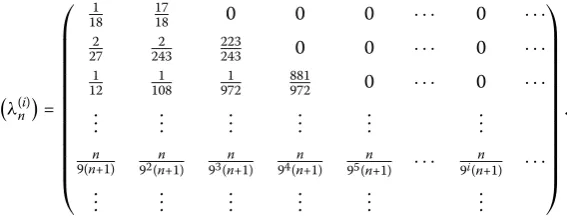
In this example, we set the parameter on{λ(ni)}byb= 9. Then we obtain

λ(_ni)= ⎛ ⎜ ⎜ ⎜ ⎜ ⎜ ⎜ ⎜ ⎜ ⎜ ⎜ ⎜ ⎜ ⎝

1 18

17

18 0 0 0 · · · 0 · · · 2

27 2 243

223

243 0 0 · · · 0 · · · 1

12 1 108

1 972

881

972 0 · · · 0 · · · ..

. ... ... ... ... ...

n 9(n+1)

n

92₍_n₊₁₎ ₉3₍_nn₊₁₎ ₉4₍_nn₊₁₎ ₉5₍_nn₊₁₎ · · · ₉i₍_nn₊₁₎ · · ·

..

. ... ... ... ... ...

⎞ ⎟ ⎟ ⎟ ⎟ ⎟ ⎟ ⎟ ⎟ ⎟ ⎟ ⎟ ⎟ ⎠ .

Figure 1 indicates the behavior ofxnfor algorithm (4.2), which converges to the same solution, that is, 0∈as a solution of this example.

Now, we test the eﬀect of the parameters in{λ(ni)}on the convergence of algorithm (4.2). In this test, Figure 2 presents the behavior ofxnby choosing three diﬀerent parameters in {λ(ni)}, that is,b= 2,b= 9, andb= 100.

5 Conclusions

(16)

Figure 2Behaviors ofxnwith three diﬀerent parameters in{λ(ni)}

for solving a class of split generalized equilibrium problems and ﬁxed point problems for a countable family of nonexpansive multivalued mappings in real Hilbert spaces.

Funding

This work was supported by the Research Center for Pure and Applied Mathematics, Research and Development Institute, Nakhon Pathom Rajabhat University, Nakhon Pathom, Thailand.

Competing interests

The authors declare that they have no competing interests.

Authors’ contributions

Both authors contributed equally and signiﬁcantly in writing this paper. Both authors read and approved the ﬁnal manuscript.

Publisher’s Note

Springer Nature remains neutral with regard to jurisdictional claims in published maps and institutional aﬃliations.

Received: 12 September 2017 Accepted: 1 February 2018

References

1. Ceng, L.C., Yao, J.C.: A hybrid iterative scheme for mixed equilibrium problems and ﬁxed point problems. J. Comput. Appl. Math.214, 186–201 (2008)

2. Blum, E., Oettli, W.: From optimization and variational inequalities to equilibrium problems. Math. Stud.63, 123–145 (1994)

3. Combettes, P.I., Hirstoaga, S.A.: Equilibrium programming in Hilbert spaces. J. Nonlinear Convex Anal.6, 117–136 (2005)

4. Flam, S.D., Antipin, A.S.: Equilibrium programming using proximal-like algorithm. Math. Program.78, 29–41 (1997) 5. Censor, Y., Gibali, A., Reich, S.: Algorithms for the split variational inequality problem. Numer. Algorithms59, 301–323

(2012)

6. Reich, S., Sabach, S.: Three strong convergence theorems regarding iterative methods for solving equilibrium problems in reﬂexive Banach spaces. Contemp. Math.56, 225–240 (2012)

7. Kazmi, K.R., Rizvi, S.H.: Iterative approximation of a common solution of a split generalized equilibrium problem and a ﬁxed point problem for nonexpansive semigroup. Math. Sci.7, 1 (2013)

8. Deepho, J., Kumam, W., Kumam, P.: A new hybrid projection algorithm for solving the split generalized equilibrium problems and the system of variational inequality problems. J. Math. Model. Algorithms Oper. Res.13(4), 405–423 (2014)

9. Deepho, J., Martinez-Moreno, J., Kumam, P.: A viscosity of Cesàro mean approximation method for split generalized equilibrium, variational inequality and ﬁxed point problems. J. Nonlinear Sci. Appl.9, 1475–1496 (2016)

(17)

11. Cianciaruso, F., Marino, G., Muglia, L., Yao, Y.: A hybrid projection algorithm for ﬁnding solutions of mixed equilibrium problem and variational inequality problem. Fixed Point Theory Appl.2010, Article ID 383740 (2010)

12. Takahashi, W., Takeuchi, Y., Kubota, R.: Strong convergence theorems by hybrid methods for families of nonexpansive mappings in Hilbert spaces. J. Math. Anal. Appl.341, 276–286 (2008)

13. Kimura, Y., Nakajo, K., Takahashi, W.: Strongly convergent iterative schemes for a sequence of nonlinear mappings. J. Nonlinear Convex Anal.9, 407–416 (2008)

14. Kimura, Y.: Convergence of a sequence of sets in a Hadamard space and the shrinking projection method for a real Hilbert ball. Abstr. Appl. Anal.2010, Article ID 582475 (2010)

15. Suantai, S., Cholamjiak, P., Cho, Y.J., Cholamjiak, W.: On solving split equilibrium problems and ﬁxed point problems of nonspreading multi-valued mappings in Hilbert spaces. Fixed Point Theory Appl.2016, 35 (2016)

16. Opial, Z.: Weak convergence of the sequence of successive approximation for nonexpansive mappings. Bull. Am. Math. Soc.73, 591–597 (1967)

17. Zegeye, H., Shahzad, N.: Convergence of Mann’s type iteration method for generalized asymptotically nonexpansive mappings. Comput. Math. Appl.62, 4007–4014 (2011)

18. Suantai, S.: Weak and strong convergence criteria of Noor iterations for asymptotically nonexpansive mappings. J. Math. Anal. Appl.311, 506–517 (2005)

19. Iiduka, H., Takahashi, W.: Weak convergence theorem by Cesàro means for nonexpansive mappings and inverse-strongly monotone mappings. J. Nonlinear Convex Anal.7, 105–113 (2006)

20. Khan, A.R.: Properties of ﬁxed point set of a multivalued map. J. Appl. Math. Stoch. Anal.3, 323–331 (2005) 21. Cholamjiak, W., Suantai, S.: A hybrid method for a countable family of multivalued maps, equilibrium problems, and

variational inequality problems. Discrete Dyn. Nat. Soc.2010, Article ID 349158 (2010)

22. Martinez-Yanesa, C., Xu, H.K.: Strong convergence of the CQ method for ﬁxed point iteration processes. Nonlinear Anal.64, 2400–2411 (2006)

23. Goebel, K., Reich, S.: Uniform Convexity, Hyperbolic Geometry, and Nonexpansive Mappings. Dekker, New York (1984) 24. Nakajo, K., Takahashi, W.: Strong convergence theorems for nonexpansive mappings and nonexpansive semigroups.

J. Math. Anal. Appl.279, 372–379 (2003)

25. Ma, Z., Wang, L., Chang, S.S., Duan, W.: Convergence theorems for split equality mixed equilibrium problems with applications. Fixed Point Theory Appl.2015, 31 (2015)