Volume 2007, Article ID 79032,13pages doi:10.1155/2007/79032
Research Article
Significance of Joint Features Derived from the Modified
Group Delay Function in Speech Processing
Rajesh M. Hegde,1Hema A. Murthy,2and V. R. R. Gadde3
1Department of Electrical and Computer Engineering, University of California San Diego, San Diego, CA 92122, USA 2Department of Computer Science and Engineering, Indian Institute of Technology Madras, Chennai 600 036, India 3STAR Lab, SRI International, 333 Ravenswood Avenue, Menlo Park, CA 94025, USA
Received 1 April 2006; Revised 20 September 2006; Accepted 10 October 2006
Recommended by Climent Nadeu
This paper investigates the significance of combining cepstral features derived from the modified group delay function and from the short-time spectral magnitude like the MFCC. The conventional group delay function fails to capture the resonant structure and the dynamic range of the speech spectrum primarily due to pitch periodicity effects. The group delay function is modified to suppress these spikes and to restore the dynamic range of the speech spectrum. Cepstral features are derived from the modified group delay function, which are called the modified group delay feature (MODGDF). The complementarity and robustness of the MODGDF when compared to the MFCC are also analyzed using spectral reconstruction techniques. Combination of several spec-tral magnitude-based features and the MODGDF using feature fusion and likelihood combination is described. These features are then used for three speech processing tasks, namely, syllable, speaker, and language recognition. Results indicate that combining MODGDF with MFCC at the feature level gives significant improvements for speech recognition tasks in noise. Combining the MODGDF and the spectral magnitude-based features gives a significant increase in recognition performance of 11% at best, while combining any two features derived from the spectral magnitude does not give any significant improvement.
Copyright © 2007 Rajesh M. Hegde et al. This is an open access article distributed under the Creative Commons Attribution License, which permits unrestricted use, distribution, and reproduction in any medium, provided the original work is properly cited.
1. INTRODUCTION
Various types of features have been used in speech pro-cessing [1]. Variations on the basic spectral computation, such as the inclusion of time and frequency masking, have been used in [2–4]. The use of auditory models as the ba-sis of feature extraction has been beneficial in many sys-tems [5–9], especially in noisy environments [10]. Perhaps the most popular features used in speech recognition today are the Mel frequency cepstral coefficients (MFCCs) [11]. In conventional speech recognition systems, features are usu-ally computed from the short-time power spectrum while the short-term phase spectrum is not used. This is primar-ily because early experiments on human speech perception have indicated that the human ear is not sensitive to short-time phase. But recent experiments described in [12, 13] have indicated the usefulness of the short-time phase spec-trum in human listening tests. In this context, the short-time phase spectrum estimated via the group delay domain has been used to parameterize speech in our earlier efforts
a discussion on the significance of joint features in speech processing.
2. SIGNIFICANCE OF FEATURE COMBINATIONS
The technique of combination is widely used in statistics. The simplest method of combination involves averaging the various estimates of the underlying information. This idea is based on the hypothesis that if different estimates are sub-ject to different sources of noise, then combining them will cancel some of the errors when an averaging is done. Good examples of combining features are the works of Christensen [22] and Janin et al. [25] who have combined different fea-tures before and after the acoustic model. Other significant works on feature and likelihood combination can be found in [33–36]. A combination system works on the principle that if some characteristics of the speech signal that is de-emphasized by a particular feature are de-emphasized by an-other feature, then the combined feature stream captures complementary information present in individual features.
2.1. Feature combination before the acoustic model
The combination of features before the acoustic model has been used by Christensen [22], Okawa et al. [20], and Ellis [21], where efforts have been made to capitalize on the dif-ferences between various feature streams using all of them at once. The joint feature stream is derived in such an approach by concatenating all the individual feature streams into a sin-gle feature stream.
2.2. Likelihood combination after the acoustic model
This approach uses the technique of combining the outputs of the acoustic models. Complex techniques of combining the posteriors [22–26,33–36] have evolved. In this context, it is also worthwhile to note that if the intent is to capitalize on the complementary information in different features, the posteriors of the same classifier for individual features can be combined to achieve improved speech recognition perfor-mance.
3. THE GROUP DELAY FUNCTION AND ITS PROPERTIES
The resonances of the speech signal present themselves as the peaks of the envelope of the short-time magnitude spectrum. These resonances, often called formants, appear as transi-tions in the short-time phase spectrum. The problem with identifying these transitions is the masking of these transi-tions due to the wrapping around of the phase spectrum at multiples of 2π. The group delay function, defined as the negative derivative of phase, can be computed directly from the speech signal and has been used to extract source and sys-tem parameters [37] when the signal under consideration is a minimum phase signal. This is primarily because the magni-tude spectrum of a minimum phase signal [37] and its group delay function resemble each other.
3.1. The group delay function
Group delay is defined as the negative derivative of the Fou-rier transform phase
τ(ω)= d
θ(ω)
dω , (1)
where the phase spectrum (θ(ω)) of a signal is defined as a continuous function ofω. The Fourier transform phase and the Fourier transform magnitude are related as in [38]. The group delay function can also be computed from the signal as in [14] using
τx(ω)= Imd
logX(ω)
dω (2)
=XR(ω)YR(ω) +YI(ω)XI(ω)
X(ω)2 , (3)
where the subscripts R and I denote the real and imagi-nary parts of the Fourier transform. X(ω) and Y(ω) are the Fourier transforms ofx(n) andnx(n), respectively. The group delay functionτ(ω) can also be viewed as the Fourier transform of the weighted cepstrum [37].
3.2. Relationship between spectral magnitude and phase
The relation between spectral magnitude and phase has been discussed extensively in [38]. In [38], it has been shown that the unwrapped phase function for a minimum phase signal is given by
θ(ω)=θv(ω) + 2πλ(ω)=
n=1
c(n) sin(nω), (4)
where c(n) are the cepstral coefficients. Differentiating (4) with respect toω, we have
τ(ω)= θ
(ω)=
n=1
nc(n) cos(nω), (5)
whereτ(ω) is the group delay function. The log-magnitude spectrum for a minimum phase signalv(n) [38] is given by
lnV(ω)=c(0)
2 +
n=1
c(n) cos(nω). (6)
(4) holds, while the unwrapped phase is given by
θ(ω)=θv(ω) + 2πλ(ω)=
n=1
c(n) sin(nω) (7)
and the group delay functionτ(ω) is given by
τ(ω)= θ
(ω)=
n=1
nc(n) cos(nω). (8)
Hence the relation between spectral magnitude and phase for a maximum phase signal [38], through cepstral coefficients, is given by (4) and (7). For mixed phase signals, the relation between spectral magnitude and phase is given by two sets of cepstral coefficientsc1(n)andc2(n), as
lnX(ω)=c1(0)
2 +
n=1
c1(n) cos(nω), (9)
where lnX(ω)is the log-magnitude spectrum for a mixed phase signal and c1(n) is the set of cepstral coefficients computed from the minimum phase equivalent signal de-rived from the spectral magnitude. Similarly, the unwrapped phase is given by
θx(ω) + 2πλ(ω)=
n=1
c2(n) sin(nω), (10)
whereθx(ω) + 2πλ(ω) is the unwrapped phase spectrum for
a mixed phase signal andc2(n)is the set of cepstral coeffi -cients computed from the minimum phase equivalent signal derived from the spectral phase. Therefore, the relation be-tween spectral magnitude and phase for a mixed phase signal [38], through cepstral coefficients, is given by (9) and (10).
3.3. Issues in group delay processing of speech
The group delay functions and their properties have been discussed in [37,39]. The two main properties of the group delay functions [39] of relevance to this work are
(i) additive property; (ii) high-resolution property.
3.3.1. Additive property
The group delay function exhibits an additive property. Let
Hejω=H 1
ejω
H2
ejω, (11)
whereH1(ejω) andH2(ejω) are the responses of the two
res-onators whose product gives the overall system response. In the group delay domain, equation (11) translates to
τh
ejω=τh1
ejω+τh2
ejω, (12)
where,τh1(ejω) andτh2(ejω) correspond to the group delay
functions of H1(ejω) andH2(ejω), respectively. From (11)
and (12), we see that multiplication in the spectral domain becomes an addition in the group delay domain.
3.3.2. High-resolution property
The group delay function has a higher resolving power when compared to both the magnitude and the LP spectrum. This property is a manifestation of the spectral additive property of the group delay function. The high-resolution property of the group delay function over both the magnitude and the linear prediction spectrum has been illustrated in [39].
3.4. Significance of pitch periodicity effects
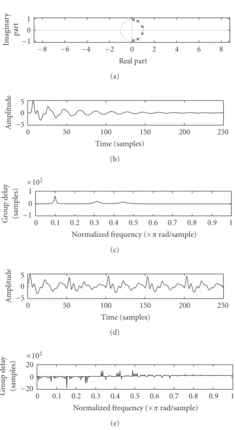
When the short-time Fourier transform power spectrum is used to extract the formants, the focus is on capturing the spectral envelope of the spectrum and not the fine structure. Similarly, the fine structure has to be deemphasized when ex-tracting the vocal tract characteristics from the group delay function. But the group delay function becomes very spiky in nature due to pitch periodicity effects. To illustrate this, a three-formant system is simulated whose pole-zero plot is shown inFigure 1(a). The formant locations are at 500 Hz, 1570 Hz, and 2240 Hz. The corresponding impulse response of the system is shown in Figure 1(b) and its group delay function is shown inFigure 1(c). The group delay function is able to resolve all the three formants. The system shown in Figure 1(a)is now excited with 5 impulses and the sys-tem response is shown inFigure 1(d). The group delay func-tion of the signal inFigure 1(d)is shown inFigure 1(e). It is evident fromFigure 1(e)that the group delay function be-comes spiky and distorted due to pitch periodicity effects. The spikes introduced into the group delay function due to zeros close to the unit circle and also due to the pitch period-icity effects form a significant part of the fine structure and cannot be removed by normal smoothing techniques. Hence the group delay function has to be modified to suppress the effects of these spikes. These considerations form the basis for modifying the group delay function.
4. THE MODIFIED GROUP DELAY FUNCTION
As mentioned in the earlier sections, for the group delay function to be a meaningful representation, it is necessary that the roots of the transfer function are not too close to the unit circle in the z plane. Normally, in the context of speech, the poles of the transfer function are well within the unit circle. The zeros of the slowly varying envelope of speech correspond to that of nasals. The zeros in speech are either within or outside the unit circle since the zeros also have nonzero bandwidth. In this section, we modify the compu-tation of the group delay function to suppress these effects. A similar approach was taken in an earlier paper by one of the authors [40] for spectrum estimation. Let us reconsider the group delay function derived directly from the speech signal. It is important to note that the denominator term
X(ω)
2in (3) becomes very small at zeros that are located
1 0 1
Im
ag
inar
y
par
t
8 6 4 2 0 2 4 6 8
Real part (a) 5
0 5
A
m
plitude
0 50 100 150 200 250
Time (samples) (b)
10 2
1 0 1
Gr
o
u
p
d
el
ay
(samples)
0 0.1 0.2 0.3 0.4 0.5 0.6 0.7 0.8 0.9 1 Normalized frequency (πrad/sample)
(c) 5
0 5
A
m
plitude
0 50 100 150 200 250
Time (samples) (d)
10 2
20 0 20
Gr
o
u
p
d
el
ay
(samples)
0 0.1 0.2 0.3 0.4 0.5 0.6 0.7 0.8 0.9 1 Normalized frequency (πrad/sample)
(e)
Figure1: Significance of pitch periodicity effects on the group delay functions (a) thez-plane with three complex poles and their com-plex conjugate pairs inside the unit circle, (b) the impulse response of the system shown in (a), (c) the group delay spectrum of the sig-nal shown in (b), (d) the response of the system shown in (a) to 5 impulses, and (e) the group delay spectrum of the signal shown in (d).
very spiky in nature and also alters the dynamic range of the group delay spectrum. The spiky nature of the group delay spectrum can be overcome by replacing the termX(ω)in the denominator of the group delay function as in (3) with its cepstrally smoothed version,S(ω).1Two new parameters γ andα are further introduced to reduce the amplitude of these spikes and to restore the dynamic range of the group
1A lower-order cepstral window lifter
wwhose length can vary from 4 to 9
is used.
delay spectrum. The new modified group delay function is defined as
τm(ω)=
τ(ω)
τ(ω)
τ(ω)α
, (13)
where
τ(ω)=
XR(ω)YR(ω) +YI(ω)XI(ω)
S(ω)2γ , (14)
whereS(ω) is the smoothed version ofX(ω). The parame-tersαandγintroduced vary from 0 to 1 where (0< α1.0) and (0< γ1.0).
Figure 2(a)shows az plane plot of a system with three resonances at 530 Hz, 1840 Hz, and 2480 Hz. In Figures2(b)
and2(c), respectively, are shown the impulse response and the group delay function of such a system. The response of the same system excited with 5 impulses and the correspond-ing group delay function are shown in Figures2(d)and2(e), respectively. The modified group delay function (lifterw =
6, α = 0.4, andγ = 0.9) for the signal in Figure 2(d) is shown inFigure 2(f). It is clear from Figures2(e)and2(f)
that while the group delay function fails to capture the for-mant structure of the signal in Figure 2(d), the modified group delay function is able to do so.
5. PARAMETERIZING THE MODIFIED GROUP DELAY FUNCTION
Since the modified group delay function exhibits a squared magnitude behavior at the location of the roots, we refer to the modified group delay function as the modified group de-lay spectra henceforth. Homomorphic processing is the most commonly used approach to convert spectrum derived from the speech signal to meaningful features. This is primarily because this approach yields features that are linearly decor-related which allows the use of diagonal covariances in mod-eling the speech vector distribution. In this context, the dis-crete cosine transform (DCT I,II,III) [41] is the most com-monly used transformation that can be used to convert the modified group delay spectra to cepstral features. Hence the group delay function is converted to cepstra using the dis-crete cosine transform (DCT II) as
c(n)=
k=Nf
k=0
τm(k) cos
n(2k+ 1)π
Nf , (15)
whereNf is the DFT order andτm(k) is the modified group
1 0 1
Im
ag
inar
y
par
t
10 8 6 4 2 0 2 4 6 8 10
Real part (a) 2
0 2
A
m
plitude
0 50 100 150 200 250
Time (samples) (b)
50 0 50
Gr
o
u
p
d
el
ay
(samples)
0 0.1 0.2 0.3 0.4 0.5 0.6 0.7 0.8 0.9 1 Normalized frequency (πrad/sample)
(c) 2
0 2
A
m
plitude
0 50 100 150 200 250 300
Time (samples) (d)
10 2
50 0 50
Gr
o
u
p
d
el
ay
(samples)
0 0.1 0.2 0.3 0.4 0.5 0.6 0.7 0.8 0.9 1 Normalized frequency (πrad/sample)
(e)
60 40 20
M
o
dified
gr
oup
dela
y
(samples)
0 0.1 0.2 0.3 0.4 0.5 0.6 0.7 0.8 0.9 1 Normalized frequency (πrad/sample)
(f)
Figure2: Comparison of the group delay and the modified group delay function to handle pitch periodicity effects. (a) Thez-plane plot of a system with three complex poles and their complex conju-gate pairs, (b) the impulse response of the system shown in (a), (c) the group delay function of the signal shown in (b), (d) the response of the system shown in (a) to 5 impulses, (e) the group delay func-tion of the signal shown in (d), and (f) the modified group delay function of the signal shown in (d).
6. SIGNIFICANCE OF SPECTRAL RECONSTRUCTIONS IN COMBINING MAGNITUDE AND
PHASE-BASED FEATURES
In this section, we reconstruct the formant structures or the respective short-time spectra from the MODGDF, MFCC,
and the joint features. The MODGDF is derived from the modified group delay spectra as
cp(n)= k=Nf
k=0
τm(k) cos
n(2k+ 1)π
Nf , (16)
whereNf is the DFT order. It is emphasized here that there
are no filter banks used in the computation of the MODGDF. The MFCC are derived from the short time power spectra as
cm(n)= k=Nf b
k=1 Xkcos
n(k 1/2)π Nf b
, (17)
wheren = 1, 2, 3,. . .,M represents the number of cepstral coefficients and k = 1, 2, 3,. . .,Nf b the number of filters
used. Xk represents the log-energy output of the kth filter.
The joint features (MODGDF + MFCC) are derived by ap-pending the MODGDF vectors calculated as in (16) with the MFCC vectors calculated as in (17). The number of cepstral coefficients used in both the MODGDF and the MFCC is the same. To reconstruct the formant structures or the short-time spectra from the cepstra, an inverse DCT of the original DFT order has to be performed on the cepstra. The recon-structed modified group delay spectra as derived from the MODGDF is given by
τm(k)= n=Nf
n=0
cp(n) cos
n(2k+ 1)π
Nf , (18)
whereNf is the DFT order, while the reconstructed
short-time power spectra derived from the MFCC is given by
Xk= n=Nf b
n=0
cm(n) cos
n(2k+ 1)π Nf b
, (19)
where n = 1, 2, 3,. . .,M represents the original number of cepstral coefficients andk = 1, 2, 3,. . .,Nf b the original
number of filters used.Xkrepresents the reconstructed
log-energy output of the kth filter. The smooth frequency re-sponse of the original DFT order is computed by interpo-lating the filter bank reconstructed energies. The short-time spectra for the joint features are reconstructed as a three-step process. First, the short-time modified group delay spec-tra of the original DFT order are reconstructed from the
n-dimensional MODGDF as in (18). Then the short-time power spectra of the original DFT order are reconstructed from then-dimensional MFCC using (19) and an interpola-tion of the resulting filter bank energies. Finally, the short-time power spectra reconstructed from the MFCC and the short-time modified group delay spectra reconstructed from the MODGDF are averaged to derive the short-time compos-ite spectra of the original DFT order. Note that the dimen-sionality of the MODGDF and the MFCC is the same.
6.1. Spectral reconstruction for a synthetic vowel
production, the transfer function of such a system is given by:
H(z)=
kbkz k
kakz k.
(20)
The transfer function of the same system for the production of vowel assuming an all pole model is given by
H(z)= k=p1
k=0akzk
, (21)
H(z)= 1 1 +kk==1pakzk
. (22)
Let the vowel be characterized by the frequenciesF1,F2,F3. Hence the poles of the system are located at
p=rejωi
. (23)
By substituting (23) in (21), the system function for produc-tion of theith formant now becomes
Hi(z)=
1 1 2rcosωiTz1+
r2z2
. (24)
But from resonance theory
r=eπBiT
. (25)
By substituting (25) in (24), the system function in (24) now becomes
Hi(z)=
1 1 2eπBiTcos
ωiTz1+
e2πBiT
z2
. (26)
In the above array of equations,ωi corresponds to the ith
formant frequency,Bi to the bandwidth of theith formant
frequency, and T to the sampling period. Using (26), we generate a synthetic vowel with the following values:F1 = 500 Hz, F2 = 1500 Hz, F3 = 3500 Hz, Bi = 10% of Fi,
andT =0.0001 second corresponding to a sampling rate of 10 KHz. Note thatF1,F2, andF3 are the formant frequen-cies in Hz. We then extract the MODGDF, MFCC, and joint features (MODGDF + MFCC) from the synthesized vowel. To reconstruct the formants, we use the algorithm described above. The reconstructed formant structures derived from the MODGDF, MFCC, joint features (MODGDF + MFCC), and also RASTA filtered MFCC are shown in Figures3(a),
3(b),3(c), and3(d), respectively. The illustrations are shown as spectrogram like plots2 where the data along theY-axis
correspond to the DFT bins and thex-axis corresponds to the frame number. It is interesting to note that while the formants are reconstructed accurately by both the MOD-GDF and the MFCC as in Figures3(a)and3(b), respectively, joint features (MODGDF + MFCC) combine the formant
2The differences between the subplots are better visualized in color than in
gray scale.
250 150 50
Fre
q
u
en
cy
(FFT
bins)
10 20 30 40 50 60 70 80 90 Frame number
0.1 0.08 0.06 0.04
(a) 250
150 50
Fre
q
u
en
cy
(FFT
bins)
10 20 30 40 50 60 70 80 90 Frame number
0.4 0.3 0.2 0.1
(b) 250
150 50
Fre
q
u
en
cy
(FFT
bins)
10 20 30 40 50 60 70 80 90 Frame number
0.25 0.15 0.05
(c) 250
150 50
Fre
q
u
en
cy
(FFT
bins)
10 20 30 40 50 60 70 80 90 Frame number
0.6 0.4 0.2 0
(d)
Figure3: Spectrogram-like plots to illustrate formant reconstruc-tions for a synthetic vowel. (a) The short-time modified group de-lay spectra reconstructed from MODGDF, (b) the short-time power spectra reconstructed from MFCC, (c) the short-time composite spectra reconstructed from joint features (MODGDF+MFCC), and (d) the short-time power spectra reconstructed from RASTA filtered MFCC.
information in the individual features as inFigure 3(c). It is expected that RASTA filtered MFCC shown in Figure 3(d)
250 200 150 100 50
Fre
q
u
en
cy
(FFT
bins)
20 40 60 80 100 120 140
Frame number (a)
250 200 150 100 50
Fre
q
u
en
cy
(FFT
bins)
20 40 60 80 100 120 140
Frame number (b)
250 200 150 100 50
Fre
q
u
en
cy
(FFT
bins)
20 40 60 80 100 120 140
Frame number (c)
Figure4: Spectrogram-like plots to illustrate formant reconstruc-tions for a synthetic speech signal with varying formant trajec-tory. (a) The short-time modified group delay spectra reconstructed from the MODGDF, (b) the short-time power spectra reconstructed from MFCC, and (c) the short-time composite spectra recon-structed from joint features (MODGDF + MFCC).
7. DATABASES USED IN THE STUDY
There are four databases used in the study. The databases used are the database for Indian languages (DBIL) for syllable recognition [27], TIMIT [28] and NTIMIT [29] for speaker identification, and OGI MLTS [32] for language identifica-tion.
7.1. The database for Indian languages (DBIL)
(i) DBIL Tamil database: this corpus consists of 20 news bulletins of the Tamil language transmitted by Door-darshan India, each of 15 minutes duration compris-ing 10 male and 10 female speakers. The total number of distinct syllables is 2184.
(ii) DBIL Telugu database: this corpus consists of 20 news bulletins of the Telugu language transmitted by Door-darshan India, each of 15 minutes duration compris-ing 10 male and 10 female speakers. The total number of distinct syllables is 1896.
7.2. The TIMIT database
The DARPA TIMIT Acoustic-Phonetic Continuous Speech Corpus was a joint effort among the Massachusetts Institute of Technology (MIT), Stanford Research Institute (SRI), and
Texas Instruments (TI). TIMIT contains a total of 6300 sen-tences, 10 sentences spoken by each of 630 speakers from 8 major dialect regions of the United States.
7.3. The NTIMIT database
The NTIMIT corpus was developed by the NYNEX Sci-ence and Technology Speech Communication Group to pro-vide a telephone bandwidth adjunct to the popular TIMIT Acoustic-Phonetic Continuous Speech Corpus. NTIMIT was collected by transmitting all the 6300 original TIMIT utter-ances through various channels in the NYNEX telephone network and redigitizing them. The actual telephone chan-nels used were varied in a controlled manner, in order to sample various line conditions. The NTIMIT utterances were time-aligned with the original TIMIT utterances so that the TIMIT time-aligned transcriptions can be used with the NTIMIT corpus as well.
7.4. The OGI MLTS database
The OGI multilanguage telephone speech corpus consists of telephone speech from 11 languages. The initial collection, included 900 calls, 90 calls each in 10 languages and was col-lected by Muthusamy et al. [32]. The languages are English, Farsi, French, German, Japanese, Korean, Mandarin, Span-ish, Tamil, and Vietnamese. It is from this initial set that the training (50), development (20), and test (20) sets were es-tablished. The National Institute of Standards and Technol-ogy (NIST) uses the same 50-20-20 set that was established. The corpus is used by NIST for the evaluation of automatic language identification.
8. FEATURE EXTRACTION AND COMBINATION
In this section, we discuss the methods for feature extraction, tuning, and combination of various features before and after the acoustic model. The features used in this work are the MFCC, the spectral root compressed MFCC (SRMFC), the energy root compressed MFCC (ERMFC), the normalized spectral root compressed MFCC (NSRMFC), the linear fre-quency cepstral coefficients (LFCC), the spectral root com-pressed LFCC (SRLFC), and the MODGDF.
8.1. Computation and tuning of spectral magnitude-based features
The speech signal is first pre-emphasized and transformed to the frequency domain using a fast Fourier transform (FFT). The frame size used is 20 ms and the frame shift used is 10 ms. A hamming window is applied on each frame of speech prior to the computation of the FFT. The frequency scale is then warped using the bilinear transformation pro-posed by Acero [42]. The frequency scale is then multiplied by a bank of filters Nf whose center frequencies are
uni-formly distributed in the interval [Minf, Maxf] along the
to another. The shape of the filter is controlled by a constant which varies from 0 to 1, where 0 corresponds to triangu-lar and 1 corresponds to rectangutriangu-lar. The filter bank energies are then computed by integrating the energy in each filter. A discrete cosine transform (DCT) is then used to convert the filter bank log energies to cepstral coefficients. Cepstral mean subtraction is always applied when working with noisy telephone speech. The front end parameters are tuned care-fully as in [43] for computing the MFCC so that the best performance is achieved. The LFCC are computed in a sim-ilar fashion except that the frequency warping is not done as in the computation of the MFCC. The velocity, acceleration, and the energy parameters are added for both the MFCC and LFCC in a conventional manner. The spectral root com-pressed MFCC are computed as described in [44] and the en-ergy root compressed MFCC as in [35]. The computation of the spectral root compressed MFCC is the same as the com-putation of the MFCC except that instead of taking a log of the FFT spectrum, we raise the FFT spectrum to a powerγ
where the value ofγranges from 0 to 2. In the computation of the energy root compressed MFCC, instead of raising the FFT spectrum to the root value, the Mel frequency filter bank energies are compressed using the root value. In the energy root compressed case, the value of the root used for com-pression can range from 0 to 1. The normalized spectral root compressed MFCC is computed by normalizing the short-time power spectrum with its cepstrally smoothed version, followed by root compression as in the case of the spectral root compressed MFCC. It is emphasized here that all the free parameters involved in the computation of all these fea-tures including the root value and the cepstral window length used in spectral smoothing have been tuned carefully so that they give the best performance and are not handicapped in any way when they are compared with the MODGDF. The values of the spectral root and the energy root used in the experiments are 2/3 and 0.08, respectively. The velocity, ac-celeration and the energy parameters are augmented to both forms of the root compressed MFCC in a conventional man-ner. Note that all free parameters in all the aforementioned features have been tuned using line search on a validation data set selected from the particular database.
8.2. Computation and tuning of free parameters for the MODGDF
There are three free parameters lifterw,α, andγinvolved in
the computation of the MODGDF as discussed inSection 4. From the results of initial experiments on the databases de-scribed inSection 7, we fix the length of the lifterw to 8
al-though the performance remains nearly the same for lengths from 4 to 9. Any value greater than 9 brings down the per-formance. Having fixed the length of the lifterw, we then
fix the values ofαandγ. In order to estimate the values of
αandγ, an extensive optimization was carried out for the SPINE database [45] for phoneme recognition. To ensure that the optimized parameters were not specific to a partic-ular database, we collected the sets of parameters that gave best performance on the SPINE database and tested them on
Table1: Series of experiments conducted on various databases with the MODGDF.
Experiments conducted on the various databases Nc=10, 12, 13, 16
γ= 0.11.0in increments of 0.1
α= 0.11.0in increments of 0.1
lifterw=4, 6, 9, 10, 12
Table2: Best front end for the MODGDF across all databases.
γ α lifterw Nc
0.9 0.4 8 13
other databases like the DBIL database (for syllable recogni-tion), TIMIT, NTIMIT (for speaker identificarecogni-tion), and the OGI MLTS database (for language identification). The val-ues of the parameters that gave the best performance across all databases and across all tasks were finally chosen for the experiments. The optimization technique uses successive line searches. For each iteration,αis held constant andγis var-ied from 0 to 1 in increments of 0.1 (line search) and the recognition rate is noted for the three tasks on the aforemen-tioned databases. The value ofγthat maximizes the recogni-tion rate is fixed as the optimal value. A similar line search is performed onα(varying it from 0 to 1 in increments of 0.1) keepingγfixed. Finally, the set of values ofαandγthat give the lowest error rate across the three tasks is retained. The series of experiments conducted to estimate the opti-mal values for lifterw,α, andγusing line search are
summa-rized inTable 1. Based on the results of such line searches, the best front end for the MODGDF across all tasks is listed inTable 2.
8.3. Extraction of joint features before the acoustic model
The following method is used to derive joint features by com-bining features before the acoustic model.
(i) Compute 13-dimensional MODGDF and the MFCC streams appended with velocity, acceleration, and en-ergy parameters.
(ii) Use feature stream combination to append the 42-dimensional MODGDF stream to the 42-42-dimensional MFCC stream to derive an 84-dimensional joint fea-ture stream.
Henceforth, we use the subscript bm for joint features thus derived.
8.4. Likelihood combination after the acoustic model
The following method is used to do a likelihood combination after the acoustic model.
(ii) Build a Gaussian mixture model (GMM) (for pho-neme, speaker, and language recognition tasks) or a hidden Markov model (HMM) (for the continuous speech recognition task).
(iii) Compute the output probability of the acoustic model for different features.
(iv) The combined output log likelihood due to different feature streams is given by
logPf = M
i=1
a(i,f)logP(i,f) (27)
and ai,f is the weight assigned to the ith feature
stream, andMis the number of feature streams used. First, a rank is assigned to the log likelihood due to each individual feature stream based on its value. The higher log likelihood value gets a higher rank. The weightsai,f are now computed as the reciprocal of the
rank assigned.
(v) Make a decision based on maximization of the com-bined output log likelihood.
Henceforth, we use the subscript am for likelihood combi-nation.Table 3summarizes the results of performance eval-uation using both feature and likelihood combination tech-niques.
9. PERFORMANCE EVALUATION
In this section, we first discuss the significance of dimension-ality of the feature vector and the size of training data. The results of performance evaluation of the MODGDF, MFCC, LFCC, NSRMFC, SRMFC, SRLFC, and joint features derived by combining these features for syllable, speaker, and lan-guage recognition are then presented. To enable a fair com-parison, the results of combining any two features derived from the short-time spectral magnitude and also the MOD-GDF are listed. Although we experimented with all possible combinations of all features, both at feature level and using likelihood combination, we present the results of combin-ing MODGDF with MFCC and MFCC with the LFCC. This is because combining any two features derived from spec-tral magnitude gave very small or no improvements, while a combination of the MODGDF with any feature derived from the spectral magnitude gave significant improvements in recognition performance. It is also noticed that new fea-tures like the NSRMFC, SRMFC, ERMFC, and SRLFC give a small improvement in recognition performance compared to the MFCC when used in isolation, but do not give any im-provement when combined with each other.
9.1. Significance of dimensionality of the feature vectors and training data
In the experimental results described in the following sec-tions, we compute a 13-dimensional vector for each feature stream appended with energy, delta, and acceleration coef-ficients. For feature combination before the acoustic mod-el, the features are concatenated to compute a joint feature
stream. Experimental results indicate that simply increas-ing the dimensionality of each individual feature stream to match the dimensionality of the joint feature stream does not improve recognition performance for any of the three tasks mentioned above. We have also experimented with increased amounts of training data for such individual high dimen-sional feature streams to validate these results. For syllable recognition, training data was increased in increments of one news bulletin from the DBIL database. For the speaker and language identification tasks, the training data was increased in increments of two sentences from the TIMIT, NTIMIT, and the OGI MLTS databases. The results from these ex-periments indicate that combining the MODGDF (derived from the short-time spectral phase) with features computed from the short-time spectral magnitude like MFCC gives an improvement in recognition performance even though the overall feature dimension is increased. It is hypothesized from these results that the MODGDF has some complemen-tary information when compared to features derived from the short-time spectral magnitude.
9.2. Syllable-based speech recognition
Table 3: Results of performance evaluation for three speech processing tasks: syllable, speaker, and language recognition for MODGDF(MGD), MFCC(MFC), LFCC(LFC), spectral root compressed MFCC(SRMFC), normalized spectral root compressed MFCC(NSRMFC), energy root compressed MFCC(ERMFC), spectral root compressed LFCC(SRLFC), MODGDF and MFCC combined be-fore the acoustic model( MGD+MFCbm), likelihood combination of MODGDF and MFCC after the acoustic model( MGD+MFCam),
MFCC and LFCC combined before the acoustic model( MFC+LFCbm), and likelihood combination of MFCC and LFCC after the acoustic
model( MFC+LFCam).
Task Feature Database Train data Test data Classifier Recog. (%) Inc. in Recog. (%)
Syllable recognition
MGD
DBIL (TELUGU)
10 news bulletins 15 mt. duration
2 news bulletins 9400 syllables
HMM 5 states 3 mixtures
36.6% —
MFC 39.6% —
LFC 32.6% —
SRMFC 35.6% —
NSRMFC 36% —
ERMFC 38% —
SRLFC 34.2% —
MGD+MFCbm 50.6% 11%
MGD+MFCam 44.6% 5%
MFC+LFCbm 41.6% 2%
MFC+LFCam 40.6% 1%
Syllable recognition
MGD
DBIL (TELUGU)
10 news bulletins 15 mt. duration
2 news bulletins 9400 syllables
HMM 5 states 3 mixtures
35.1% —
MFC 37.1% —
LFC 31.2% —
SRMFC 34.1% —
NSRMFC 34.5% —
ERMFC 36.5% —
SRLFC 32.4% —
MGD+MFCbm 48.9% 11%
MGD+MFCam 41.7% 4.6%
MFC+LFCbm 39.1% 2%
MFC+LFCam 38% 0.9%
Speaker identification
MGD
TIMIT 6 sentences/speaker 4 sentences/speaker GMM 64 mixtures
98% —
MFC 98% —
LFC 96.25% —
SRMFC 97.25% —
NSRMFC 97% —
ERMFC 98% —
SRLFC 97% —
MGD+MFCbm 99% 1%
MGD+MFCam 99% 1%
MFC+LFCbm 98% 0%
MFC+LFCam 98% 0%
Speaker identification
MGD
NTIMIT 6 sentences/speaker 4 sentences/speaker GMM 64 mixtures
41% —
MFC 40% —
LFC 30.25% —
SRMFC 34.25% —
NSRMFC 35% —
ERMFC 34.75% —
SRLFC 31.75% —
MGD+MFCbm 47% 6%
MGD+MFCam 45% 4%
MFC+LFCbm 40% 0%
Table3: Continued.
Task Feature Database Train data Test data Classifier Recog. (%) Inc. inRecog. (%)
Language identification
MGD
OGI MLTS 11-language task
45 sentences 40 males and 5 females
20 sentences 18 males and 2 females
GMM 64 mixtures
53% —
MFC 50% —
LFC 47% —
SRMFC 50.4% —
NSRMFC 50.8% —
ERMFC 50.6% —
SRLFC 48% —
MGD+MFCbm 58% 5%
MGD+MFCam 57% 4%
MFC+LFCbm 51% 1%
MFC+LFCam 50.5% 0.5%
9.3. Speaker identification
In this section, we discuss the baseline system and ex-perimental results for speaker identification on the TIMIT database (clean speech) and the NTIMIT database (noisy telephone speech). A series of GMMs modeling the voices of speakers for whom training data is available and a clas-sifier that evaluates the likelihoods of the unknown speak-ers voice data against these models make up the likelihood maximization-based baseline system used in this section. Single state, 64 mixture Gaussian mixture models (GMMs) are trained for each of the 630 speakers in the database. The number of sentences used for training each speaker’s model is 6, while 4 sentences are used to test a particu-lar speaker during the testing phase. Hence a total of 400 tests are conducted to identify 100 speakers and the num-ber of tests goes up to 2520 for identifying 630 speakers. For the TIMIT (clean speech) data [28], the MODGDF (MGD) recognition performance was at 98%, MFCC (MFC) at 98%, (MGD+MFCbm) at 99%, and (MGD+MFCam) at 99% for this task. The best increase due to feature combination was 1%. While for the NTIMIT (noisy telephone speech) data [29], the MODGDF (MGD) recognition performance was at 41%, MFCC (MFC) at 40%, (MGD+MFCbm) at 47%, and (MGD+MFCam) at 45% for this task. The best increase due to feature combination was 6% as indicated in
Table 3. The results for combining the MODGDF with the LFCC are also tabulated inTable 3and show minor improve-ments.
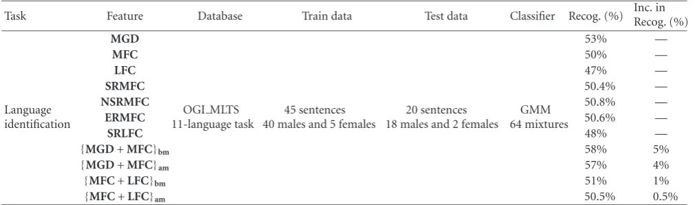
9.4. Language identification
In this section, we discuss the baseline system and experi-mental results for language identification on the OGI MLTS database (11-language task for noisy telephone speech). The baseline system used for this task is very similar to the sys-tem used for the automatic speaker identification task as in
Section 9.3, except that each language is now modeled by a GMM. From the 90 phrases available for each language, 45 are used for training and 20 are used for testing. The du-ration of the test utterance is 45 seconds. The results of the MODGDF and the MFCC on the OGI MLTS [32] corpora
using the GMM scheme are listed in Table 3. For the 11-language task on the OGI MLTS data, the MODGDF (MGD) recognition performance was at 53%, MFCC (MFC) at 50%, (MGD+MFCbm) at 58%, and (MGD+MFCam) at 57% for this task. The best increase due to feature combination was 5%. The results for combining the MODGDF with the LFCC are also tabulated inTable 3, and indicate that combin-ing two spectral magnitude-based features does not give sig-nificant improvements for the language identification task. It was also noticed from the confusion matrix created from our recognition experiments that Japanese and Korean had a high degree of confusion between themselves, and that the MODGDF was able to identify Korean better, while the MFCC performed better in recognizing Japanese.
10. CONCLUSION
the performance evaluation indicate the complementarity of the MODGDF to the MFCC, it is not clear how a measure of complementarity can be defined. The use of feature pruning techniques like the sequential floating forward search with appropriate distance measures to reduce the dimensionality of the joint feature stream is another issue that needs to be addressed.
ACKNOWLEDGMENT
The work of Rajesh M. Hegde was supported by the Na-tional Science Foundation under Award numbers 0331707 and 0331690—http://www.itr-rescue.org.
REFERENCES
[1] L. R. Rabiner and B. H. Juang,Fundamentals of Speech Recog-nition, Prentice Hall, Englewood Cliffs, NJ, USA, 1993. [2] K. Aikawa, H. Singer, H. Kawahara, and Y. Tohkura, “A
dy-namic cepstrum incorporating time-frequency masking and its application to continuous speech recognition,” in Proceed-ings of IEEE International Conference on Acoustics, Speech, and Signal Processing (ICASSP ’93), vol. 2, pp. 668–671, Minneapo-lis, Minn, USA, April 1993.
[3] M. Bacchiani and K. Aikawa, “Optimization of time-frequency masking filters using the minimum classification error crite-rion,” inIEEE International Conference on Acoustics, Speech, and Signal Processing (ICASSP ’94), vol. 2, pp. 197–200, Ade-laide, SA, Australia, April 1994.
[4] H. Hermansky, “Perceptual linear predictive (PLP) analysis of speech,”Journal of the Acoustical Society of America, vol. 87, no. 4, pp. 1738–1752, 1990.
[5] O. Ghitza, “Auditory models and human performance in tasks related to speech coding and speech recognition,”IEEE Trans-actions on Speech and Audio Processing, vol. 2, no. 1, part 2, pp. 115–132, 1994.
[6] K. L. Payton, “Vowel processing by a model of the auditory pe-riphery: a comparison to eighth-nerve responses,”The Journal of the Acoustical Society of America, vol. 83, no. 1, pp. 145–162, 1988.
[7] R. Lyon, “A computational model of filtering, detection, and compression in the cochlea,” inProceedings of IEEE Interna-tional Conference on Acoustics, Speech, and Signal Processing (ICASSP ’82), vol. 7, pp. 1282–1285, Paris, France, May 1982. [8] S. Seneff, “A joint synchrony/mean-rate model of auditory
speech processing,”Journal of Phonetics, vol. 16, no. 1, pp. 55– 76, 1988.
[9] J. R. Cohen, “Application of an auditory model to speech recognition,”The Journal of the Acoustical Society of America, vol. 85, no. 6, pp. 2623–2629, 1989.
[10] M. J. Hunt, S. M. Richardson, D. C. Bateman, and A. Piau, “An investigation of PLP and IMELDA acoustic representa-tions and of their potential for combination,” inProceedings of IEEE International Conference on Acoustics, Speech, and Sig-nal Processing (ICASSP ’91), vol. 2, pp. 881–884, Toronto, Ont, Canada, May 1991.
[11] S. B. Davis and P. Mermelstein, “Comparison of paramet-ric representations for monosyllabic word recognition in con-tinuously spoken sentences,”IEEE Transactions on Acoustics, Speech, and Signal Processing, vol. 28, no. 4, pp. 357–366, 1980. [12] K. K. Paliwal and L. D. Alsteris, “On the usefulness of STFT phase spectrum in human listening tests,”Speech Communica-tion, vol. 45, no. 2, pp. 153–170, 2005.
[13] L. D. Alsteris and K. K. Paliwal, “Some experiments on iter-ative reconstruction of speech from STFT phase and magni-tude spectra,” inProceedings of 9th European Conference on Speech Communication and Technology (EUROSPEECH ’05), pp. 337–340, Lisbon, Portugal, September 2005.
[14] H. A. Murthy and V. R. R. Gadde, “The modified group delay function and its application to phoneme recognition,” in Pro-ceedings of IEEE International Conference on Acoustics, Speech, and Signal Processing (ICASSP ’03), vol. 1, pp. 68–71, Hong Kong, April 2003.
[15] R. M. Hegde, H. A. Murthy, and V. R. R. Gadde, “Applica-tion of the modified group delay func“Applica-tion to speaker identi-fication and discrimination,” inProceedings of IEEE Interna-tional Conference on Acoustics, Speech, and Signal Processing (ICASSP ’04), vol. 1, pp. 517–520, Montreal, Quebec, Canada, 2004.
[16] R. M. Hegde, H. A. Murthy, and V. R. R. Gadde, “Continuous speech recognition using joint features derived from the mod-ified group delay function and MFCC,” inProceedings of 8th International Conference on Spoken Language Processing (IN-TERSPEECH ’04), vol. 2, pp. 905–908, Jeju Island, Korea, Oc-tober 2004.
[17] R. M. Hegde, H. A. Murthy, and V. R. R. Gadde, “The modified group delay feature: a new spectral representation of speech,” inProceedings of 8th International Conference on Spoken Lan-guage Processing (INTERSPEECH ’04), vol. 2, pp. 913–916, Jeju Island, Korea, October 2004.
[18] R. M. Hegde, H. A. Murthy, and V. R. R. Gadde, “Significance of the modified group delay feature in speech recognition,” to appear inIEEE Transactions on Speech and Audio Processing. [19] R. M. Hegde, H. A. Murthy, and V. R. R. Gadde, “Speech
processing using joint features derived from the modified group delay function,” in Proceedings of IEEE International Conference on Acoustics, Speech, and Signal Processing (ICASSP ’05), vol. 1, pp. 541–544, Philadelphia, Pa, USA, March 2005.
[20] S. Okawa, E. Bocchieri, and A. Potamianos, “Multi-band speech recognition in noisy environments,” inProceedings of the IEEE International Conference on Acoustics, Speech, and Sig-nal Processing (ICASSP ’98), vol. 2, pp. 641–644, Seattle, Wash, USA, May 1998.
[21] D. Ellis, “Feature stream combination before and/or after the acoustic model,” Tech. Rep. TR-00-007, International Com-puter Science Institute, Berkeley, Calif, USA, 2000.
[22] H. Christensen, “Speech recognition using heterogenous in-formation extraction in multi-stream based systems,” Ph.D. dissertation, Aalborg University, Aalborg, Denmark, 2002. [23] B. E. D. Kingsbury and N. Morgan, “Recognizing
reverber-ant speech with RASTA-PLP,” inProceedings of IEEE Interna-tional Conference on Acoustics, Speech, and Signal Processing (ICASSP ’97), vol. 2, pp. 1259–1262, Munich, Germany, April 1997.
[24] S.-L. Wu, B. E. D. Kingsbury, N. Morgan, and S. Greenberg, “Incorporating information from syllable-length time scales intoautomatic speech recognition,” inProceedings of the IEEE International Conference on Acoustics, Speech, and Signal Pro-cessing (ICASSP ’98), vol. 2, pp. 721–724, Seattle, Wash, USA, May 1998.
[26] K. Kirchhoffand J. A. Bilmes, “Dynamic classifier combina-tion in hybrid speech recognicombina-tion systems using utterance-level confidence values,” in Proceedings of IEEE Interna-tional Conference on Acoustics, Speech, and Signal Processing (ICASSP ’99), vol. 2, pp. 693–696, Phoenix, Ariz, USA, March 1999.
[27] Database for Indian Languages, Speech and Vision Lab, IIT Madras, Chennai, India, 2001.
[28] NTIS, The DARPA TIMIT Acoustic-Phonetic Continuous Speech Corpus, 1993.
[29] C. Jankowski, A. Kalyanswamy, S. Basson, and J. Spitz, “NTIMIT: a phonetically balanced, continuous speech, tele-phone bandwidth speech database,” inProceedings of IEEE In-ternational Conference on Acoustics, Speech, and Signal Process-ing (ICASSP ’90), vol. 1, pp. 109–112, Albuquerque, NM, USA, April 1990.
[30] L. Besacier and J. F. Bonastre, “Time and frequency pruning for speaker identification,” inProceedings of the 14th Interna-tional Conference on Pattern Recognition (ICPR ’98), vol. 2, pp. 1619–1621, Brisbane, Qld., Australia, August 1998.
[31] K. L. Brown and E. B. George, “CTIMIT: a speech cor-pus for the cellular environment with applications to auto-matic speech recognition,” in Proceedings of IEEE Interna-tional Conference on Acoustics, Speech, and Signal Processing (ICASSP ’95), vol. 1, pp. 105–108, Detroit, Mich, USA, May 1995.
[32] Y. K. Muthusamy, R. A. Cole, and B. T. Oshika, “The OGI multi-language telephone speech corpus,” inProceedings of the 2nd International Conference on Spoken Language Processing (ICSLP ’92), pp. 895–898, Banff, Alberta, Canada, October 1992.
[33] K. Turner, “Linear and order statistics combiners for reliable pattern classification,” Ph.D. dissertation, University of Texas at Austin, Austin, Tex, USA, May 1996.
[34] M. P. Perrone and L. N. Cooper, “When networks disagree: ensemble methods for hybrid neural networks,” inNeural Net-works for Speech and Image Processing, pp. 126–142, Chapman-Hall, London, UK, 1993.
[35] R. Sarikaya and J. H. L. Hansen, “Analysis of the root-cepstrum for acoustic modeling and fast decoding in speech recog-nition,” in Proceedings of the 7th European Conference on Speech Communication and Technology (EUROSPEECH ’01), pp. 687–690, Aalborg, Denmark, September 2001.
[36] A. Krogh and J. Vedelsby, “Neural network ensembles, cross validation, and active learning,” inAdvances in Neural Infor-mation Processing Systems, vol. 7, pp. 231–238, MIT Press, Cambridge, Mass, USA, 1995.
[37] H. A. Murthy and B. Yegnanarayana, “Formant extraction from group delay function,”Speech Communication, vol. 10, no. 3, pp. 209–221, 1991.
[38] B. Yegnanarayana, D. K. Saikia, and T. R. Krishnan, “Signifi-cance of group delay functions in signal reconstruction from spectral magnitude or phase,”IEEE Transactions on Acous-tics, Speech, and Signal Processing, vol. 32, no. 3, pp. 610–623, 1984.
[39] V. K. Prasad, T. Nagarajan, and H. A. Murthy, “Automatic seg-mentation of continuous speech using minimum phase group delay functions,”Speech Communication, vol. 42, no. 3-4, pp. 429–446, 2004.
[40] B. Yegnanarayana and H. A. Murthy, “Significance of group delay functions in spectrum estimation,”IEEE Transactions on Signal Processing, vol. 40, no. 9, pp. 2281–2289, 1992.
[41] P. Yip and K. R. Rao,Discrete Cosine Transform: Algorithms, Advantages, and Applications, Academic Press, San Diego, Calif, USA, 1997.
[42] A. Acero, “Acoustical and environmental robustness in auto-matic speech recognition,” Ph.D. dissertation, Carnegie Mel-lon University, Pittsburgh, Pa, USA, 1990.
[43] H. A. Murthy, F. Beaufays, L. P. Heck, and M. Weintraub, “Ro-bust text-independent speaker identification over telephone channels,”IEEE Transactions on Speech and Audio Processing, vol. 7, no. 5, pp. 554–568, 1999.
[44] P. Alexandre and P. Lockwood, “Root cepstral analysis: a uni-fied view. Application to speech processing in car noise envi-ronments,”Speech Communication, vol. 12, no. 3, pp. 277–288, 1993.