A PREDICTIVE MODEL FOR ESTIMATING PETROLEUM CONSUMPTION
USING MACHINE LEARNING APPROACH
Folorunso, S. O., Taiwo, A. I.
*, Olabanjo, O. E.
Department of Mathematical Sciences, Olabisi Onabanjo University, Ago Iwoye
*Corresponding author: [email protected]
ABSTRACT
This study is focused on predicting the consumption of Petroleum (Thousands of Barrels per year) in Nigeria. Autoregressive integrated moving average (ARIMA), Linear Regression (LR) and Random Forest Regression (RFR) models were fitted to predict the consumption of Petroleum. The prediction accuracy of these models was evaluated using Root Mean Square Error (RMSE), Mean Absolute Error (MAE), Mean Absolute Percentage Error (MAPE) and Coefficient of determination( )metrics. The Petroleum dataset spanned a period of 37 years (1980-2017) and it was spilted into train and test at the ratio of 70:30 respectively to reduce overfitting. The result obtained revealed that the two machine learning models: LR and RFR outperformed the ARIMA model with lower values
of prediction accuracy in terms of MAE, MAPE, RMSE and
R
2.Keywords: Energy and Oil Consumption; Prediction Accuracy; Regression; Forecasting, Time Series
INTRODUCTION
Access to clean energy is one of the essential factors used to meet basic needs of people and it stimulate and support economic growth which in turn improve the level of standard of living (Oyedepo, 2012). The consumption of Petroleum is erratic and has increased sharply in the recent past years (Hymel, 2006). The scarcity in the supply of Petroleum products has increased greatly and has affected the prices and the distribution of Petroleum products (Nnabuife et al.,, 2016). The trend which the factors mentioned above has followed on the distribution of Petroleum was triggered by lack of appropriate prediction model to proffer predictions for the future consumption of Petroleum based on the past observations made on the consumption of petroleum (Oyedepo, 2012).
The severity of energy problems has made energy issues and policies urgent and necessary to be synthesized within an integrated framework at the national level (Omer, 2012). Omer (2012) also observed that energy consumptions are characterized by extremely high levels of price volatility of a market that are influenced by the cost of production. He identified energy as a critical input to the economy which should be given policy priority to ensure its adequate supply in order to support a stable and sound economy. The fundamental issue that needs to be addressed in energy planning is scarcity and
consumption of Petroleum products. Global demand for Petroleum is expected to grow and many researchers and practitioners have proposed many models of global oil consumption using various fundamental, technical and analytical techniques to give a more or less exact prediction (Bhattacharyya and Timilsina, 2009).
predict electricity consumption in Nigeria. The data was divided into train, validation and test sets in the ratio of 13:3:4 respectively to avoid overfitting. RBF performed better than equivalent Back-Propagation (BP) network models when compared based on training time (Time), Sum of Square Error (SSE), Mean Square Error (MSE) and correlation coefficient (R). Bonetto and Rossi (2017) used SVM, Recurrent Neural Network (RNN) and ARIMA models to fit and predict residential energy consumption time series data. The result they obtained indicated that SVM and RNN had smaller prediction errors in the mean and variance when compared to ARMA. Seyedzadeh, Rahimian, Glesk, & Roper, (2018) gave a comprehensive review four main machine learning
clustering to forecasting and improving building energy performance on time series data. In-essence, this paper is aimed at building a machine learning predictive model LR and RFR for estimating and predicting petroleum consumption in Nigeria. In addition, the predictive efficiency of LR, RFR and ARIMA will be determine using RMSE, MAE, MAPE and Coefficient of determination (R2).
MATERIALS AND METHODS
The methods employed for forecasting of Petroleum consumption will be Box-Jenkins ARIMA and Machine Learning Models: LR and RFR. Figure 1 described the methodology adopted for the prediction of Petroleum consumption.
Figure 1. Petroleum Consumption Modeling Process
Dataset
The Nigerian Yearly Petroleum Consumption dataset analysed in this research was obtained from
http://nigeria.opendataforafrica.org/ovfhfrg/total-petroleum-consumption-1980-2018. The date of the observations ranges from 1980 to 2017 (37 years). The features contain the date and the value on consumption in thousands of barrels per year. The experiment was setup at the R Studio (RStudio, 2012) and programmed with R language (R Core Team, 2013). Packages implemented were Forecast Packages (Hyndman and Khandakar, 2008), “TSA” , “party” (Strobl et al., 2008), “random Forest” (Liaw and Wiene, Classification and Regression by randomForest, 2002), LR (Grömping, 2006) and ARIMA (Hyndman & Khandakar, 2008) were used for the prediction of petroleum Consumption in Nigeria. This experiment was performed on a Workstation with an Intel processor of 3.0 GHz, 4GB of Random-Access Memory, VGA with desktop performance for windows, 320GB hard disk.
Models
This section will describe the models employed for the forecast and the parameters used.
Box-Jenkins ARIMA Model
Autoregressive Moving average model relate what happens in period t to both the past values and the random errors that occurred in past time periods (Box and Jenkins, 1976). A general ARMA model can be written as follow
= ∅ + ∅ + ⋯ + ∅ + + + + ⋯ + (1)
Equation (1) can be simplified by a backward shift operator to obtain
( )∇ = ( ) (2)
and can be written as ( , , )where ∇ =
(1 − ) with∇ and consecutive differencing. Steps involved in ARIMA model building is illustrated in Figure 2.
Figure 2. The Box-Jenkins Model stages
Model Identification for ARIMA Model
Autocorrelations function (ACF) and partial autocorrelation functions (PACF) are the two most useful tools in time series model identification. This was used to identify the AR and MA parts of the ARIMA model. Differencing based on unit root test was also applied to determine the order of integrated which maybe level, first and second differences. The identified models was validated using Akaike Information (AIC) and Bayesian information criteria (BIC) respectively.
Parameter Estimation for ARIMA Model
After choosing the most appropriate model, ordinary least square (OLS) estimation method will be used to estimate the coefficients of the model. For the OLS method, a time series model given as
= ∅ + , = 1, … , (3)
will be considered. Then the OLS estimator of ∅ is given by
∅ =∑∑ (4)
Diagnostic Checking for ARIMA Model
A careful analysis of the estimated residuals will be carried out by checking whether the residuals are white noise and this is done by computing the sample ACF and PACF of the residuals to see whether they do not form any pattern and all are statistically significant, that is, within two standard deviation with
= 0.05.
vector (instances and features) as data for modelling. Consequently, the trained model is applied to an unseen similar data for prediction or classification. This process is known as supervised learning. The supervised learning models considered in this research are linear regression and random forest regression models
Linear Regression (LR) Model
Linear Regression refers to a group of techniques for fitting and studying the straight-line relationship between two variables. Linear regression estimates the regression coefficients and as modeled in by (5)
= + + (5)
X is the independent variable, Y is the dependent variable, is the Y intercept, is the slope, and ε is
the error (NCSS Statistical Software, 2000).
Random Forest Regression (RFR)
Random Forests (Breiman, 2001) is a variant of Bagging (Breiman, 1996) but with an extra coat of randomness. In addition to constructing each tree using a different bootstrap sample of the data, random forests change how the classification or regression trees are constructed. In standard trees, each node is split using the best split among all variables. In a random forest, each node is split using the best among a subset of predictors randomly chosen at that node. This somewhat counterintuitive strategy turns out to perform very well compared to many other classifiers, including discriminant analysis, support vector machines and neural networks, and is robust against
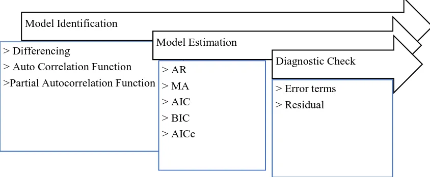
Model Identification
> Differencing
> Auto Correlation Function
>Partial Autocorrelation Function
Model Estimation
> AR
> MA
> AIC
> BIC
> AICc
Diagnostic Check
Random Forest is represented in (6)
( ) = ( ) + ( ) + ( ) + ⋯ (6)
where the final model g is the sum of simple base models fi. Here, each base classifier is a simple decision tree, all the base models are constructed independently using a different subsample of the data.
Forecast Evaluation Metrics
The accuracy of the forecast of each model used in the research will be measured using Mean Absolute Error (MAE) defined as
=ℎ + 11 ( − ) (7)
Root Mean Square Error (RMSE) defined as
= ℎ + 11 ( − ) (8)
the Mean Absolute Percentage Error (MAPE) defined as
=ℎ +100 − (9)
and Coefficient of determination ( )defined as
= 1 − (10)
ℎ = , 1 + , … ,ℎ+ . The actual and
predicted values for corresponding values are denoted by respectively. SSE is the sum of square of error and SST is the sum of square of total.
RESULTS AND DISCUSSION
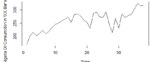
From the time plot of the petroleum consumption in Figure 3, there is a continuous increasing trend and some fluctuation points. This indicate non-stationarity of the series and differencing order 2 up to was used to attain stationarity. The differenced dataset was divided into two (train and test data) with the ratio of 70:30 respectively in order to rightly fit the ARIMA, LR and RFR models. The autocorrelation function (ACF) and partial autocorrelation function (PACF) plots in Figure 4-5 were used to determine the order of the AR part and MA part of the ARIMA (p, d, q) model. The Autocorrelation Function (ACF) plot indicated that the series is normalized and cut-off at lag 2. This is an indication that = 1 2 and a further investigate in-term of partial autocorrelation function (PACF) in Figure 5 indicated that the series decay exponentially to at lag 2. Therefore, can be taken as 1or 2 respectively. In-hence, the tentative model can be ARIMA (1,1,1), ARIMA (2.1.2), ARIMA (2,1,1) and ARIMA (1,1,2). After estimation, based on the smallest values of AIC and BIC, ARIMA (1,1,1) was chosen as the optimal model. The ACF, PACF plot of the residual and Ljung-Box Statistic in figure 6 indicated that the residual of ARIMA (1,1,1) is white noise and this indicated that ARIMA (1,1,1) is suitable for model and predicting Nigerian yearly petroleum consumption.
Figure 4. Autocorrelation Plot for Nigerian Petroleum consumption
Figure 5. Partial Autocorrelation plot of Nigerian Petroleum consumption
Figure 6. ACF, PACF Residual plots and Ljung-Box Statistic
Analysis based on the Metrics
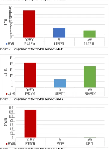
The differenced dataset was divided into train and test data in the ratio of 70:30 respectively and evaluated on the three models. The result obtained based on the evaluation of the models are illustrated in Figures 7-10. Evaluating the four models on MAE metric, ARIMA, LR and RFR have error estimates of 16.3407, 5.8213 and 4.3616 respectively. With RMSE metric, it
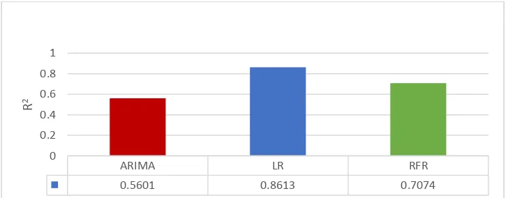
based on the value of R2 of LR at 0.8613, RFR at 0.7074 and ARIMA (1,1,1) at 0.5601, the variation in
with linear regression model.
Figure 7: Comparison of the models based on MAE
Figure 8: Comparison of the models based on RMSE
Figure 9: Comparison of the models based on MAPE
ARIMA LR RFR
MAE 16.34069 5.821264 4.361564 0
2 4 6 8 10 12 14 16 18
MAE
ARIMA LR RFR
RMSE 20.98975 7.020655 17.80237 0
5 10 15 20 25
RMS
E
ARIMA LR RFR
MAPE 130.0914 0.2911 1.1655 0
20 40 60 80 100 120 140
MAP
Figure 10: Comparison of the models based on R2
CONCLUSION
It has been reported in the literatures that machine learning models can perform very well on time series forecasting. In this paper, we propose LR and RFR for predicting petroleum consumption in Nigeria and compared the result with ARIMA. The four phases involved the machine learning models for time series forecasting: data collection, dataset preprocessing (Differencing), training and learning and test forecasting. An empirical study, in which we compare LR and RFR’s performance with ARIMA (1,1,1) is put underway to verify the effectiveness of the machine learning models based on MAE, RMSE, MAPE and R2. The results show that LR is superior to RFR and ARIMA forecasting methods in the yearly Nigerian petroleum consumption prediction. The prediction can be improved if the parameters of the machine learning models were tuned.
REFERENCES
(NESP), N. E. (2015). The Nigerian Energy Sector: An Overview with a Special Emphasis on Renewable Energy, Energy Efficiency and Rural Electrification (2nd ed.). Deutsche Gesellschaft für Internationale
Zusammenarbeit (GIZ) GmbH.
Bhattacharyya, S. C., Timilsina, G. R. (2009). Energy Demand Models for Policy: A Comparative Study of Energy Demand Models.
Bonetto, R., Rossi, M. (2017). Machine Learning Approaches to Energy Consumption Forecasting in Households. 1-4.
Box, G. P., Jenkins, G. M. (1976). Time series analysis: Forecasting and control. Rev. San
Retrieved February 17, 2018, from
https://link.springer.com/content/pdf/10.102 3/A:1018054314350.pdf
Breiman, L. (2001). Random forests. Machine Learning, 45(1), 5-32. Retrieved February 16, 2018, from
https://www.stat.berkeley.edu/~breiman/ran domforest2001.pdf
Folorunso, O., Akinwale, A. T., Asiribo, O. E., Adeyemo, T. A. (2010). Population prediction using artificial neural network. African Journal of Mathematics and Computer Science Research, 3(8):155- 162.
Grömping, U. (2006). Relative Importance for Linear Regression in R: The Package relaimpo. . Journal of Statistical Software, 17(1):1-27.
Hymel, M. L. (2006). Globalisation, Environmental Justice and Sustainable Development: The case of oil. Macquarie Law Review, 29. Retrieved from
https://ssrn.com/abstract=934467
Hyndman, R. J., Khandakar, Y. (2008). Automatic time series forecasting: the forecast package for R. Journal of Statistical Software, 26(3):1-22.
Liaw, A., Wiene, M. (2002). Classification and Regression by randomForest. R News, 2(3):18-22.
Liaw, A., Wiener, M. (2002). Classification and Regression by Random Forest. R News, 2(3):18-22.
ARIMA LR RFR
0.5601 0.8613 0.7074 0
0.2 0.4 0.6 0.8 1
R
ssl.com/wp-content/themes/ncss/pdf/Procedures/NCSS/ Linear_Regression_and_Correlation.pdf
Nnabuife, E. K., Orogbu, L. O., Onyeizugbe, C. U., Onyilofor, T. U. (2016). Fuel Scarcity and Business Growth in NIgeria from 2005 to 2015. European Journal of Business, Economics and Accountancy, 4(8):9-31.
Omer, A. M. (2012). The Energy Crisis, the Role of Renewable and Global Warming. Greener Journal of Environment Management and Public Safety, 1(1):38-70.
Oyedepo, S. O. (2012). Energy and sustainable development in Nigeria: the way forward. Energy, Sustainability and Society, 2(15):1-17.
R Core Team. (2013). R: A language and environment for statistical computing. R Foundation for Statistical Computing, Vienna, Austria. Retrieved from URL http://www.R-project.org/
RStudio. (2012, May 20). RStudio: Integrated development environment for R (Version 0.96.122). Computer software.
(2018). Machine learning for estimation of building energy consumption and
performance: A review. Visualization in Engineering, 6(5). doi:s40327-018-0064-7
Strobl, C., Boulesteix, A.-L., Kneib, T., Augustin, T., Zeileis, A. (2008). Conditional Variable Importance for Random Forests. . BMC Bioinformatics, 9(307). Retrieved from http://www.biomedcentral.com/1471-2105/9/307
Usman, O. L., Folorunso, O., Alaba, O. B. (2016). Electricity Consumption Prediction System using a Radial basis function neural network. Journal of Natural Science, Engineering and Technology, 15(1):1-20.