Computing Mixed-Design (Split-Plot) ANOVA »

Computing Mixed-Design

(Split-Plot) ANOVA

Sylvain Chartier

Denis Cousineau

The mixed, within-between subjects ANOVA (also called a split-plot ANOVA) is a statistical test of means commonly used in the behavioral sciences. One approach to computing this analysis is to use a corrected between-subjects ANOVA. A second approach uses the general linear model by partitioning the sum of squares and cross-product matrices. Both approaches are detailed in this article. Finally, a package called MixedDesignANOVA is

introduced that runs mixed-design ANOVAs using the second approach and displays summary statistics as well as a mean plot.

‡

Introduction

The mixed, within-between subjects design (also called split-plot or randomized blocks factorial) ANOVA is a technique that compares the means obtained by manipulating two factors, one being a repeated-measure factor. Let g be the number of independent groups, each representing one level of the between-subjects factor, let c be the number of meas-ures corresponding to the within-subjects factor, and let ni be the number of subjects in

The data is contained in a matrix X of the form:

X

=

1

y

y

º⋯

y

1

y

y

º⋯

y

ª

ª

ª

ª

1

y

y

º⋯

y

2

y

y

º⋯

y

2

y

y

º⋯

y

ª

ª

ª

ª

2

y

y

º⋯

y

ª

ª

ª

ª

g yg

yg

º⋯

yg

g yg

yg

º⋯

yg

ª

ª

ª

ª

g ygn

ygn

º⋯

ygn

First load the package. It is available from

www.mathematica-journal.com/data/uploads/2011/10/Chartier.zip.

Needs@"MixedDesignANOVA`"D

An example taken from Howell [1] (p. 481) concerns data collected in a study by King [2]. King investigated the effect of midazolam on the motor activity of rats. The rats were measured at six different times (c=6) and there were g=3 equal groups of ni=8

WSLabels=8"Time", 8"t1", "t2", "t3", "t4", "t5", "t6"<<; BSLabels=8"Group", 8"Control", "Same", "Different"<<; X=8

81, 150., 44., 71., 59., 132., 74.<,

81, 335., 270., 156., 160., 118., 230.<,

81, 149., 52., 91., 115., 43., 154.<,

81, 159., 31., 127., 212., 71., 224.<,

81, 159., 0., 35., 75., 71., 34.<,

81, 292., 125., 184., 246., 225., 170.<,

81, 297., 187., 66., 96., 209., 74.<,

81, 170., 37., 42., 66., 114., 81.<,

82, 346., 175., 177., 192., 239., 140.<,

82, 426., 329., 236., 76., 102., 232.<,

82, 359., 238., 183., 123., 183., 30.<,

82, 272., 60., 82., 85., 101., 98.<,

82, 200., 271., 263., 216., 241., 227.<,

82, 366., 291., 263., 144., 220., 180.<,

82, 371., 364., 270., 308., 219., 267.<,

82, 497., 402., 294., 216., 284., 255.<,

83, 362., 104., 144., 114., 115., 127.<,

83, 338., 132., 91., 77., 108., 169.<,

83, 282., 186., 225., 134., 189., 169.<,

83, 317., 31., 85., 120., 131., 205.<,

83, 263., 94., 141., 142., 120., 195.<,

83, 138., 38., 16., 95., 39., 55.<,

83, 329., 62., 62., 6., 93., 67.<,

83, 292., 139., 104., 184., 193., 122.< < ê.81->BSLabelsP2, 1T, 2->BSLabelsP2, 2T,

3->BSLabelsP2, 3T<; TableForm@X,

Group t1 t2 t3 t4 t5 t6

Control 150. 44. 71. 59. 132. 74.

Control 335. 270. 156. 160. 118. 230.

Control 149. 52. 91. 115. 43. 154.

Control 159. 31. 127. 212. 71. 224.

Control 159. 0. 35. 75. 71. 34.

Control 292. 125. 184. 246. 225. 170.

Control 297. 187. 66. 96. 209. 74.

Control 170. 37. 42. 66. 114. 81.

Same 346. 175. 177. 192. 239. 140.

Same 426. 329. 236. 76. 102. 232.

Same 359. 238. 183. 123. 183. 30.

Same 272. 60. 82. 85. 101. 98.

Same 200. 271. 263. 216. 241. 227.

Same 366. 291. 263. 144. 220. 180.

Same 371. 364. 270. 308. 219. 267.

Same 497. 402. 294. 216. 284. 255.

Different 362. 104. 144. 114. 115. 127.

Different 338. 132. 91. 77. 108. 169.

Different 282. 186. 225. 134. 189. 169.

Different 317. 31. 85. 120. 131. 205.

Different 263. 94. 141. 142. 120. 195.

Different 138. 38. 16. 95. 39. 55.

Different 329. 62. 62. 6. 93. 67.

Different 292. 139. 104. 184. 193. 122.

Ú Table 1. Data from Howell (2003) of a 3×6 design (three groups, six repeated measures).

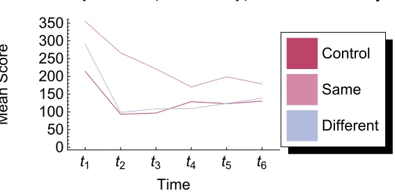
The plot of the means across conditions (Figure 1) shows evidence of a time effect, the re-sults on the second time being generally smaller than those on the first time. In addition, there is an interaction effect caused by the “same” group that does not follow this pattern.

MeanPlotê. MixedDesignANOVA@X,

Labels->8WSLabels, BSLabels<, MeanPlotØTrueD

t1 t2 t3 t4 t5 t6

0 50 100 150 200 250 300 350

Time

Mean

Score

Different Same Control

Ú Figure 1. Illustration of the example given in Table 1.

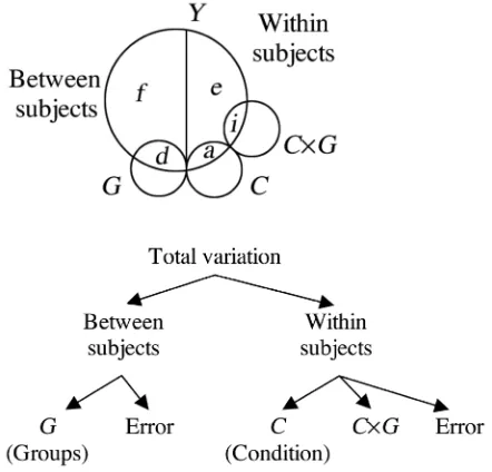
Figure 2 shows variation partitioning for the subjects by condition design. The between-subjects variation is decomposed into two parts: a source of variation due to the group effect (area d) and a source of variation due to the measurement error (area f). Within-subjects variation is decomposed into three areas: a source of variation for the repeated measures effect (area a), a source of variation for the interaction between the repeated measures and the group effect (area i), and a source of variation for error (area e). Conse-quently, there will be three F ratios to compute: the group effect (the ratio fêd, FG), the

repeated measure effect (the ratio aêe, FC) and the interaction effect (the ratio iêe, FCµG).

Ú Figure 2. (top) Venn diagram for the subjects within groups by conditions design. G is the group ef-fect, C is the repeated-measure effect and CµG is the interaction effect between the two factors. (bottom) Tree diagram showing the partitioning of the different sources of variation.

The total variation R2 _{is 1=a+d+e+ f+i . Each letter corresponds to a proportion of} variation (r-squared). The between-subjects proportions of variation are:

d=R_Y2_ÿG,

f =R_Y2_ÿS-R_Y2_ÿG,

d+ f =R_Y2_ÿS,

where R_Y2_{ÿS represents the variation explained by the between-subjects source. By dividing}

d and f by d+ f, we get the mean effect, that is, the group effect:

d

d+f =RYÿG

2 _,

f

d+f =1 -d

d+ f =1-RYÿG

Finally, the within-subjects proportions of variation are:

a=R_Y2_ÿC,

i=R_Y2_ÿCµG,

e=1-Hd+fL-a-i=1-R2_YÿS-R_Y2_ÿC-R_Y2_ÿCµG.

The various F statistics are ratios of the following proportions of variation weighted by their corresponding degrees of freedom:

FG= d

f µ N-g

g-1 =

R_Y2_ÿG

1-R_Y2_ÿG µ

N-g

g-1,

FC= a

e µN-g=

R_Y2_ÿC

1-R_Y2_ÿS-R YÿC

2 _-R

YÿCµG

2 µN-g,

FCµG= i

eµ N-g

g-1 =

R_Y2_ÿCµG

1-R_Y2_ÿS-R YÿC

2 _-R

YÿCµG

2 µ

N-g

g-1.

‡

Computing a Split-Plot ANOVA from the Computations

Obtained by a Between-Subjects ANOVA

·

Test of the Between-Subjects Effect

The group (between-subjects) effect (measured by dêf in Figure 2) can be obtained by averaging the repeated measures (so that information about the repeated measures is discarded) and submitting them to a one-way ANOVA:

y_{i j}= 1

c ‚ k=1 c

y_{i jk},i=1, …,g, j=1, …,ni.

Using Mathematica, we need to set a few constants first, and for convenience, the labels for the within- and between-subjects factors. The conditions are taken from the first col-umn of X.

AllConditions=Union@XPAll, 1TD;

This computes the number of groups and repeated measures.

This computes the total number of participants and the number of participants per group.

nTotal=Length@XD; Table@

ni =Length@Select@XPAll, 1T, Ò ==AllConditionsPiT&DD,

8i, 1, g<D;

Finally, we define the labels.

WSLabels=8"Time", 8"t1", "t2", "t3", "t4", "t5", "t6"<<; BSLabels=8"Group", 8"Control", "Same", "Different"<<; WSVariable=Time;

BSVariable=Group;

To get the between-subjects effect, we aggregate the data over replicated measures.

y_G=TableB:XPj, 1T, 1

c Total@Drop@XPjT, 1DD>, 8j, nTotal<F;

Using this, a one-way ANOVA is computed.

Needs@"ANOVA`"D

resGrp=ANOVA@y_G, 8BSVariable<, 8BSVariable<, CellMeansØFalseD

ANOVAØ

DF SumOfSq MeanSq FRatio PValue Group 2 47 635.8 23 817.9 7.80059 0.00292823 Error 21 64 120.3 3053.35

Total 23 111 756.

In the following, we will need the between-subjects sum of squares, so we extract it from the table. To take into account the c repeated measures, the sum of squares must be multi-plied by that number of measures.

SSBetween=c µ resGrpP2, 1, 3, 2T

·

Test of the Within-Subjects Effect

F ratios for the repeated-measure effect and the interaction effect are computed by first re-coding the data matrix such that the repeated measures look like a second between-sub-jects factor. Thus, the bulk of the analysis simplifies into a standard factorial ANOVA. The following transforms the data.

yCµG=Flatten@Table@8XPj, 1T, i, XPj, i+1T<,8i, c<,

8j, nTotal<D, 1D;

Applying a standard between-factors ANOVA, the following summary table is obtained.

results=ANOVA@yCµG,8WSVariable, BSVariable, All<,

8WSVariable, BSVariable<, CellMeansØFalseD

ANOVAØ

DF SumOfSq MeanSq FRatio PValue

Time 2 285 815. 142 908. 27.0398 1.69471µ10-10

Group 5 399 737. 79 947.3 15.127 1.26463µ10-11

Group Time 10 80 820. 8082. 1.52921 0.136377

Error 126 665 921. 5285.09

Total 143 1.43229µ106

First, the results regarding the group effect are discarded since it has been analyzed in the previous section. Next, the results regarding the repeated measure “time” and the inter-action (group × time) must be modified to obtain the corrected F ratios. Specifically, infor-mation regarding the error term is incorrect since it does not take into account the estimation of the between-subjects error that we obtained in the previous subsection. The corrected error sum of squares is given by

SSError=SSTotal-SSBetween-SSWithin-SSinteraction.

The corrected error degrees of freedom (df) is given by

dfError =HN-gL Hc-1L.

Using the results of the previous ANOVA, the sum of squares terms can be extracted and the corrected error term computed.

SSTotal=resultsP2, 1, 5, 2T; SSWithin=resultsP2, 1, 2, 2T; SSInteraction=resultsP2, 1, 3, 2T;

SSError=SSTotal-SSBetween-SSWithin-SSInteraction;

dfError=HnTotal-gLµHc-1L

From this, the error mean square (MS) can be computed.

MSError=

SSError

dfError

2678.09

The within-subjects F ratios are summarized in the following table.

TableForm@8

Join@resultsP2, 1, 2, 81, 2, 3<T,

8resultsP2, 1, 2, 3T êMSError,

1-CDF@FRatioDistribution@resultsP2, 1, 1, 1T, dfErrorD, resultsP2, 1, 1, 3T êMSErrorD<D,

Join@resultsP2, 1, 3, 81, 2, 3<T,

8resultsP2, 1, 3, 3T êMSError,

1-CDF@FRatioDistribution@resultsP2, 1, 3, 1T, dfErrorD, resultsP2, 1, 3, 3T êMSErrorD<D,

8dfError, SSError, MSError< <,

TableHeadingsØ

88WSLabelsP1T, WSLabelsP1T<>" µ "<>BSLabelsP1T, "Error"<,

8"DF", "SS", "MS", "F", "P"<< D

DF SS MS F P

Time 5 399 737. 79 947.3 29.8524 1.11022µ10-16

Time µ Group 10 80 820. 8082. 3.01782 0.00216428 Error 105 281 199. 2678.09

‡

Computing a Split-Plot ANOVA Using the General Linear

Model Approaches

·

Test of the Between-Subjects Effect

For this effect, a coding matrix that identifies each subject within each group could be used. However, as pointed out in [3] and detailed in [4], it is simpler to aggregate the repeated measures as in the previous section to consider only the group effect. Hence, the effect coding matrix for the groups (ECG) has g lines. Because the last group is entirely

determined by the other groups, it is not coded (otherwise the resulting matrix would be singular), resulting in g-1 columns.

Group Coded As x1 x2 º⋯ xg-1

1 Ø 1 0 º⋯ 0

2 Ø 0 1 º⋯ 0

ª ª ª ª ¸⋱ ª

g-1 Ø 0 0 º⋯ 1

g Ø -1 -1 º⋯ -1

Using the group coding vector for each subject and joining to it the dependent variable, we get a matrix M that contains the predictor variables in the first columns and the depen-dent variable in the last column.

With this matrix M, the sum of squares and cross-product (SSCP) matrix can be com-puted by

(1) SSCP=M¬M-H1¬ML¬H1¬ML êN,

where 1 represents the N-dimensional vector composed of 1s. By partitioning the SSCP matrix, the coefficient of determination R2 _{is obtained. The SSCP must be partitioned into} four submatrices named SSpp, SSpd, SSd p, and SSdd (in which the subscript p stands for predictors and d stands for dependent variable). These matrices represent, respectively, the sum of squares of the predictors alone, the sum of cross-products between the predic-tors and the dependent variable, the sum of cross-products between the dependent variable and the predictors, and lastly the sum of squares of the dependent variable alone.

SSCP=

SSpp SSpd

SS_{d p} SS_dd ,

where the size of the SSpp matrix is Hg-1LµHg-1L and the size of the SSdd matrix is

1µ1. Finally, we verify that SS_pd=SS_{d p}¬.

The coefficient of determination for the between-subjects effect (R_Y2_{ÿG) can be obtained by} the matrix multiplication

Finally, the F value is the ratio between the explained variation and the unexplained varia-tion, weighted by the degrees of freedom:

FG= R

YÿG 2

1-R_Y2_ÿG

µ N-g

g-1.

All those operations are performed with the following commands. First we have the cod-ing matrix.

ECG=Append@Table@AllConditionsPiTØIdentityMatrix@g-1DPiT,

8i, g-1<D,

AllConditionsPgTØTable@-1, 8g-1<DD; TableForm@ECGD

ControlØ81, 0< DifferentØ80, 1< SameØ8-1,-1<

The means for each group are then computed.

y_G=TableB:XPj, 1T, 1

c Total@Drop@XPjT, 1DD>, 8j, nTotal<F

88Control, 88.3333<, 8Control, 211.5<, 8Control, 100.667<, 8Control, 137.333<, 8Control, 62.3333<,8Control, 207.<, 8Control, 154.833<, 8Control, 85.<, 8Same, 211.5<,

8Same, 233.5<,8Same, 186.<, 8Same, 116.333<, 8Same, 236.333<, 8Same, 244.<, 8Same, 299.833<,

8Same, 324.667<, 8Different, 161.<, 8Different, 152.5<, 8Different, 197.5<, 8Different, 148.167<,

8Different, 159.167<, 8Different, 63.5<, 8Different, 103.167<, 8Different, 172.333<<

Then the matrix M can be constructed.

M=Map@Flatten@8ÒP1T ê. ECG,ÒP2T<D&, yGD

881, 0, 88.3333<, 81, 0, 211.5<, 81, 0, 100.667<, 81, 0, 137.333<, 81, 0, 62.3333<, 81, 0, 207.<, 81, 0, 154.833<, 81, 0, 85.<,8-1, -1, 211.5<,

8-1, -1, 233.5<, 8-1, -1, 186.<, 8-1,-1, 116.333<, 8-1, -1, 236.333<, 8-1,-1, 244.<, 8-1, -1, 299.833<, 8-1, -1, 324.667<, 80, 1, 161.<, 80, 1, 152.5<,

From this matrix M, the SSCP matrix is easily obtained according to equation 1.

ones=Array@1 &, 8Length@MD, 1<D; [email protected]

-Transpose@[email protected]@onesD.ML ê

Length@MD; MatrixForm@SSCPD

16. 8. -805.167

8. 16. -694.833

-805.167 -694.833 111 756.

This SSCP matrix can then be partitioned into the various sum of squares submatrices needed to compute R

YÿG

2 _.

SSpp=Take@SSCP,81, g-1<,81, g-1<D; SSpd=Take@SSCP,81, g-1<,8g, g<D; SSdd=Take@SSCP,8g, g<, 8g, g<D;

R2_YÿG =ITransposeASSpdE.InverseASSppE.SSpd.Inverse@SSddDMP

1, 1T

0.426248

Finally, the F ratio can be obtained.

FG= R2YÿG 1-R2_YÿG µ

nTotal-g

g-1

7.80059

And again, the total sum of squares of the between-subjects factor S_Y2 is memorized for later use (area f in Figure 2).

SSBetween=c µ SSdd;

·

Test of the Within-Subjects Effects

The first step is to compute the proportion of variance accounted for by the repeated measure effect R_Y2_{ÿC. To this end, we must create an effect coding matrix for the c repeated} measures. This effect coding is created as in the previous section except that it is of size c.

ECC=Append@

Table@iØIdentityMatrix@c-1DPiT, 8i, c-1<D, cØTable@-1, 8c-1<DD;

TableForm@ECCD

1Ø81, 0, 0, 0, 0< 2Ø80, 1, 0, 0, 0< 3Ø80, 0, 1, 0, 0< 4Ø80, 0, 0, 1, 0< 5Ø80, 0, 0, 0, 1<

6Ø8-1, -1, -1, -1,-1<

The raw data is reorganized so that for each item, the replication number is available,

9j,yi jk=, i=1, …,g, j=1, …,c, and k=1, …ni. From it, the matrix M is computed in

ex-actly the same way as before.

yC=Flatten@Table@8i, XPj, i+1T<, 8i, 1, c<, 8j, nTotal<D, 1D; M=Map@Flatten@8ÒP1T ê. ECC, ÒP2T<D&, yCD;

Next, the SSCP matrix is computed exactly as before.

ones=Array@1 &, 8Length@MD, 1<D; [email protected]

-Transpose@[email protected]@onesD.ML ê

Length@MD; MatrixForm@SSCPD

48. 24. 24. 24. 24. 3290.

24. 48. 24. 24. 24. 83.

24. 24. 48. 24. 24. -171. 24. 24. 24. 48. 24. -318. 24. 24. 24. 24. 48. -19. 3290. 83. -171. -318. -19. 1.43229µ106

Partitioning this matrix, the quantity R_Y2_{ÿC can be obtained exactly as before.}

SSpp=Take@SSCP,81, c-1<,81, c-1<D; SSpd=Take@SSCP,81, c-1<,8c, c<D; SSdd=Take@SSCP,8c, c<, 8c, c<D;

R2YÿC =ITransposeASSpdE.InverseASSppE.SSpd.Inverse@SSddDMP 1, 1T

The same steps are repeated one last time for the interaction effect R_Y2ÿCµG. The effect

cod-ing matrix for the interaction is defined for all the combinations of the between-subjects factor and the repeated-measure factor. It is obtained with the outer product of the individ-ual effect coding.

ECCG=Flatten@

Table@8AllConditionsPjT, i<Ø

Flatten@Transpose@8AllConditionsPjT ê. ECG<D.

H8iê. ECC<LD, 8j, 1, g<, 8i, 1, c<D, 1D;

TableForm@ECCGD

8Control, 1<Ø81, 0, 0, 0, 0, 0, 0, 0, 0, 0< 8Control, 2<Ø80, 1, 0, 0, 0, 0, 0, 0, 0, 0< 8Control, 3<Ø80, 0, 1, 0, 0, 0, 0, 0, 0, 0< 8Control, 4<Ø80, 0, 0, 1, 0, 0, 0, 0, 0, 0< 8Control, 5<Ø80, 0, 0, 0, 1, 0, 0, 0, 0, 0<

8Control, 6<Ø8-1, -1, -1, -1, -1, 0, 0, 0, 0, 0< 8Different, 1<Ø80, 0, 0, 0, 0, 1, 0, 0, 0, 0< 8Different, 2<Ø80, 0, 0, 0, 0, 0, 1, 0, 0, 0< 8Different, 3<Ø80, 0, 0, 0, 0, 0, 0, 1, 0, 0< 8Different, 4<Ø80, 0, 0, 0, 0, 0, 0, 0, 1, 0< 8Different, 5<Ø80, 0, 0, 0, 0, 0, 0, 0, 0, 1<

8Different, 6<Ø80, 0, 0, 0, 0, -1, -1, -1, -1,-1< 8Same, 1<Ø8-1, 0, 0, 0, 0, -1, 0, 0, 0, 0<

The data matrix is reorganized one last time so that both the group and the number of the repeated measures are available: 9i, j,y_{i jk}=, i=1 , …,g, j=1, …,c, and k=1, …ni. The M and SSCP matrices are then computed as usual.

yCG=Flatten@Table@8XPj, 1T, i, XPj, i+1T<, 8i, 1, c<,

8j, nTotal<D, 1D;

M=Map@Flatten@88ÒP1T, ÒP2T< ê. ECCG, ÒP3T<D&, yCGD;

ones=Array@1 &, 8Length@MD, 1<D; [email protected]

-Transpose@[email protected]@onesD.ML ê

Length@MD; MatrixForm@SSCPD

32. 16. 16. 16. 16. 16. 8. 8. 8. 8. -738. 16. 32. 16. 16. 16. 8. 16. 8. 8. 8. -996. 16. 16. 32. 16. 16. 8. 8. 16. 8. 8. -608. 16. 16. 16. 32. 16. 8. 8. 8. 16. 8. 57. 16. 16. 16. 16. 32. 8. 8. 8. 8. 16. -218. 16. 8. 8. 8. 8. 32. 16. 16. 16. 16. -196. 8. 16. 8. 8. 8. 16. 32. 16. 16. 16. -1024. 8. 8. 16. 8. 8. 16. 16. 32. 16. 16. -580. 8. 8. 8. 16. 8. 16. 16. 16. 32. 16. -168. 8. 8. 8. 8. 16. 16. 16. 16. 16. 32. -281. -738. -996. -608. 57. -218. -196. -1024. -580. -168. -281. 1.43229µ106

Partitioning this last matrix, the quantity R_Y2_ÿCµG can be obtained.

SSpp=Take@SSCP,81, Hg-1L Hc-1L<, 81,Hg-1L Hc-1L<D; SSpd=Take@SSCP,81, Hg-1L Hc-1L<,

8Hg-1L Hc-1L+1, Hg-1L Hc-1L+1<D;

SSdd=Take@SSCP,8Hg-1L Hc-1L+1, Hg-1L Hc-1L+1<,

8Hg-1L Hc-1L+1, Hg-1L Hc-1L+1<D;

R2YÿCµG =ITransposeASSpdE.InverseASSppE.SSpd.Inverse@SSddDMP 1, 1T

Finally, the error proportion of variance can be estimated as the within-subjects variation left unexplained:

R2_Error=1-R_Y2_ÿS-R2_YÿC-R_Y2_ÿCµG,

in which R_Y2_ÿS is given by

R_Y2ÿS= S

Y 2

S_Y2,

where S_Y2 _{is the between-factors sum of squares memorized in the previous subsection.}

R2YÿS =

SSBetween

SSdd P1, 1T

0.468156

R2Error=1-R2YÿS-R2YÿC-R2YÿCµG

0.196328

The F ratios for the repeated-measure effect and the interaction effect can be computed with the formulas:

FC= R_Y2_ÿC

R_Error2

µHN-gL,

F_CµG=

R_Y2_ÿCµG

R_Error2 µ

N-g

g-1,

which we compute.

FC= R2YÿC

R2Error HnTotal-gL

29.8524

FCG= R2YÿCµG R2Error

nTotal-g

g-1

3.01782

‡

The MixedDesignANOVA Package

The MixedDesignANOVA package performs the different analyses using the procedures outlined in the previous section. It works for equal as well as for unequal numbers of sub-jects per group. To use it, first load the package (adapt the path if necessary) and load some data. Optionally, you can define labels for the factors and the levels of the factors.

Needs@"MixedDesignANOVA`"D

X=88Control, 150., 44., 71., 59., 132., 74.<,

8Control, 335., 270., 156., 160., 118., 230.<,

8Control, 149., 52., 91., 115., 43., 154.<,

8Control, 159., 31., 127., 212., 71., 224.<,

8Control, 159., 0., 35., 75., 71., 34.<,

8Control, 292., 125., 184., 246., 225., 170.<,

8Control, 297., 187., 66., 96., 209., 74.<,

8Control, 170., 37., 42., 66., 114., 81.<,

8Same, 346., 175., 177., 192., 239., 140.<,

8Same, 426., 329., 236., 76., 102., 232.<,

8Same, 359., 238., 183., 123., 183., 30.<,

8Same, 272., 60., 82., 85., 101., 98.<,

8Same, 200., 271., 263., 216., 241., 227.<,

8Same, 366., 291., 263., 144., 220., 180.<,

8Same, 371., 364., 270., 308., 219., 267.<,

8Same, 497., 402., 294., 216., 284., 255.<,

8Different, 282., 186., 225., 134., 189., 169.<,

8Different, 317., 31., 85., 120., 131., 205.<,

8Different, 362., 104., 144., 114., 115., 127.<,

8Different, 338., 132., 91., 77., 108., 169.<,

8Different, 263., 94., 141., 142., 120., 195.<,

8Different, 138., 38., 16., 95., 39., 55.<,

8Different, 329., 62., 62., 6., 93., 67.<,

8Different, 292., 139., 104., 184., 193., 122.<<; WSLabels=8"times",8"t1", "t2", "t3", "t4", "t5", "t6"<<;

The command MixedDesignANOVA, with a data matrix respecting the input format X

defined in the first section, displays the ANOVA table only, with default names (B for the between-subjects factor and A for the within-subjects factor).

ANOVATableê. MixedDesignANOVA@XD

SC dl CM F P

Between-Subjects

B 285 815. 2 142 908. 7.80059 0.00292823 Error 384 722. 21 18 320.1

Total 670 537. 23

Within-Subjects

A 399 737. 5 79 947.3 29.8524 5.43708µ10-11 A µ B 80 820. 10 8082. 3.01782 0.00216428 Error 281 199. 105 2678.09

Total 761 756. 120

Total 1.43229µ106 143

The command has seven options, as listed below. The option Epsilons is used to compute the Greenhouse–Geisser, the Huynh–Feldt and the lower-bound epsilons [5, 6]. The options MeanTable and MeanPlot show the mean across conditions and measures under the form of a table or visually. The option VarCov returns the gµg variance-covariance matrices for each group as well as the global variance-variance-covariance matrix.

Finally, the option SummaryStatistics can be used to display summary statistics for each cell of the design. Default summary statistics are None; Automatic returns the mean, variance, standard deviation, length (i.e. the number of observations in the cell), un-biased skewness, and unun-biased kurtosis.

Options@MixedDesignANOVAD

8ANOVATableØTrue, EpsilonsØFalse,

LabelsØAutomatic, MeanPlotØFalse, MeanTableØFalse, SummaryStatisticsØNone, VarCovØFalse<

The next command runs an analysis with all options turned on; the results are displayed one at a time afterward.

analysis=MixedDesignANOVA@X, LabelsØ8WSLabels, BSLabels<, MeanPlotØFalse, MeanTableØTrue,

SummaryStatisticsê. analysis

Mean Total Variance Skewness Control-t1 213.875 1711. 6274.41 0.57759

Control-t2 93.25 746. 8699.93 0.933113

Control-t3 96.5 772. 2927.14 0.452598

Control-t4 128.625 1029. 4943.98 0.638305

Control-t5 122.875 983. 4256.41 0.503268

Control-t6 130.125 1041. 5557.27 0.199142

Control 130.875 6282. 6490.66 0.614616

Same-t1 354.625 2837. 8084.55 -0.211362

Same-t2 266.25 2130. 12 031.4 -0.677922

Same-t3 221. 1768. 4883.43 -0.969977

Same-t4 170. 1360. 6100.86 0.406149

Same-t5 198.625 1589. 4385.41 -0.554247

Same-t6 178.625 1429. 6987.98 -0.644123

Same 231.521 11 113. 10 434.2 0.213016

Different-t1 290.125 2321. 4805.55 -1.36696

Different-t2 98.25 786. 2859.64 0.21114

Different-t3 108.5 868. 3926.57 0.465401

Different-t4 109. 872. 2759.14 -0.688462

Different-t5 123.5 988. 2510.29 -0.0230334

Different-t6 138.625 1109. 3137.7 -0.374307

Different 144.667 6944. 7468.31 0.83978

Grand total 169.021 24 339. 10 016. 0.63334

MeanTableê. analysis

t1 t2 t3 t4 t5 t6 Mean

Control 213.875 93.25 96.5 128.625 122.875 130.125 130.875

Same 354.625 266.25 221. 170. 198.625 178.625 231.521

Different 290.125 98.25 108.5 109. 123.5 138.625 144.667

Mean 286.208 152.583 142. 135.875 148.333 149.125 169.021

Epsilonsê. analysis

VarCovê. analysis

:

VarianceêCovariance matrices Hone per groupL ,

:

6274.41 6929.32 2512.21 2386.38 3604.13 2123.16 6929.32 8699.93 2688.57 1933.96 3123.75 3045.68 2512.21 2688.57 2927.14 3462.36 1188.21 3413.64 2386.38 1933.96 3462.36 4943.98 1212.8 4183.63 3604.13 3123.75 1188.21 1212.8 4256.41 -444.982 2123.16 3045.68 3413.64 4183.63 -444.982 5557.27

,

8084.55 6094.11 2564. 188.429 990.411 2144.41 6094.11 12 031.4 7233.86 4323.14 3591.54 6710.25 2564. 7233.86 4883.43 3169. 2978. 4478.57 188.429 4323.14 3169. 6100.86 3876.57 3695.71 990.411 3591.54 2978. 3876.57 4385.41 1982.41 2144.41 6710.25 4478.57 3695.71 1982.41 6987.98

,

4805.55 1065.25 1644.21 -529.857 1458.64 1504.63 1065.25 2859.64 2622. 1128. 1959.29 839.679 1644.21 2622. 3926.57 1458.71 2318.86 2001.07

-529.857 1128. 1458.71 2759.14 1656.43 1374.43 1458.64 1959.29 2318.86 1656.43 2510.29 1430.5 1504.63 839.679 2001.07 1374.43 1430.5 3137.7

>,

VarianceêCovariance common matrix

,

6388.17 4696.23 2240.14 681.649 2017.73 1924.07 4696.23 7863.64 4181.48 2461.7 2891.52 3531.87 2240.14 4181.48 3912.38 2696.69 2161.69 3297.76 681.649 2461.7 2696.69 4601.33 2248.6 3084.59 2017.73 2891.52 2161.69 2248.6 3717.37 989.31 1924.07 3531.87 3297.76 3084.59 989.31 5227.65

,

The two unbiased functions are available as SkewnessU@listD and KurtoÖ

sisU@listD following the formulas given in [7].

?? SkewnessU

SkewnessU@listDcomputes the unbiased skewness over the list.

SkewnessU@list_D:= nHn-1L Skewness@listD

n-2 ê. nØLength@listD

?? KurtosisU

KurtosisU@listDcomputes the unbiased kurtosis excess over the list.

KurtosisU@list_D:=

HHn-1L Hn+1LLKurtosis@listD Hn-2L Hn-3L

-3Hn-1L2

Hn-2L Hn-3L ê. nØLength@listD

The package MixedDesignANOVA works in Mathematica 4.0 and higher. It is available with this article or can be found at

www.mapageweb.umontreal.ca/cousined/home/Others/MixedDesignAnova/Index.html.

‡

References

[1] D. C. Howell, Fundamental Statistics for the Behavioral Sciences, 5th ed., Belmont, CA: Thomson–Brooks/Cole, 2004.

[2] D. A. King, “Associative Control of Tolerance to the Sedative Effects of a Short-Acting Benzo-diazepine,” unpublished doctoral dissertation, University of Vermont, 1986.

[3] J. Cohen and P. Cohen, Applied Multiple Regression/Correlation Analysis for the Behavioral Sciences, 2nd ed., Hillsdale, NJ: Lawrence Erlbaum Associates, 1983.

[4] A. L. Edwards, Multiple Regression and the Analysis of Variance and Covariance, 2nd ed., New York: W. H. Freeman, 1985.

[5] S. W. Greenhouse and S. Geisser, “On Methods in the Analysis of Profile Data,” Psychome-trika, 24(2), 1959 pp. 95–112. www.springerlink.com/content/220512x5l554733q.

[6] H. Huynh and L. S. Feldt, “Estimation of the Box Correction for Degrees of Freedom from Sample Data in the Randomized Block and Split Plot Designs,” Journal of Educational Statis-tics, 1(1), 1976 pp. 69–82. www.jstor.org/pss/1164736.

About the Authors

Sylvain Chartier is a professor of cognitive psychology and quantitative methods at the University of Ottawa. His areas of research include artificial neural networks and nonlin-ear dynamic systems applied to psychology.

Denis Cousineau is a professor of cognitive psychology at the University of Ottawa. He runs research in artificial intelligence as well as on human categorization processes.

Sylvain Chartier

School of Psychology University of Ottawa 136 Jean Jacques Lussier Ottawa, Ontario

K1N 6N5, Canada

[email protected]

Denis Cousineau

School of Psychology University of Ottawa 136 Jean Jacques Lussier Ottawa, Ontario

K1N 6N5, Canada