A COMPARATIVE STUDY OF SOME ESTIMATORS IN ECONOMETRIC MODEL WITH MULTICOLLINEARITY.

[Badawaire* 5(2): February, 2018] ISSN 2349-4506

Impact Factor: 3.799

G

lobal

J

ournal of

E

ngineering

S

cience and

R

esearch

M

anagement

A COMPARATIVE STUDY OF SOME ESTIMATORS IN ECONOMETRIC MODEL

WITH MULTICOLLINEARITY

Abdulrasheed BelloBadawaire*, S. Y. Jackson, M. G. Bukar

* Department of Mathematics & Statistics, Federal University Wukari, P.M.B. 1020, Wukari, Nigeria Department of Mathematical Sciences, University of Maiduguri, Maiduguri, Nigeria

Department of Basic Science, MohametLawan College of Agriculture Maiduguri, P.M.B. 1427, Maiduguri, Nigeria

DOI: 10.5281/zenodo.1186509

KEYWORDS

:

ABSTRACT

Mostly, economic data are afflicted with the problems of multicollinearity. This leads to inaccurate parameter estimates in Ordinary Least Squares. Therefore, this paper examined the efficiency of three methods of parameter estimation in regression model (Ordinary Least Squares(OLS), Ridge Regression and Least Absolute Shrinkage and Selection Operator (LASSO)) under multicollinearity. Monte-Carlo experiment of 1000 trials was carried out for four sample sizes (20, 50, 100 and 150), each with three levels of collinearity( Low, Mild and Severe). The findings from this paper showed that when the collinearity level between the predictors is low, irrespective of the sample size, OLS is the most efficient estimator. However, under mild or severe collinearity condition, irrespective of the sample size, Lasso is the most efficient estimator.

INTRODUCTION

Multicollinearity is one of the problems in computing the Ordinary Least Squares estimates in regression analysis. It occurs when the assumption of ‘‘no linear dependencies among the predictor variables’’ is violated. It can as well be defined as a situation whereby two or more of the explanatory variables considered in a model are related (Belsley, 1991; Murray, 2006).

Multicollinearity can be perfect or inperfect. A situation occurs whereby two or more predictors considered in a model move exactly in step with each other and is called a perfect multicollinearity condition (Mrray, 2006). If multicollinearity is perfect, the regression coefficients of the X variables are indeterminate and their standard errors are infinite (Gujarati, 2004). When the multicollinearity in the data is inperfect, the linear combination of the relevant columns, though not zero, is small (Stewart, 1987).

Multicollinearity comes into a model through the data collection method employed, model specification errors, constraints on the model or in the population being sampled, over determination of a model and so on (Gujarati, 2004).

Multicollinearity creates improper specification and inflation of variances of the coefficient estimates (Alin, 2010; Murray, 2006).

When the assumptions of classical linear regression model are met, Least Squares estimator has minimum variance (Stock & Watson, 2007). However, if multicollinearity exists in a data, the OLS estimators, though may still be linear, unbiased, and asymptotically normally distributed, would no longer have the minimum variance among linear unbiased estimators, and as such, would be inefficient relative to other linear unbiased estimators.

[Badawaire* 5(2): February, 2018] ISSN 2349-4506

Impact Factor: 3.799

G

lobal

J

ournal of

E

ngineering

S

cience and

R

esearch

M

anagement

MATERIALS AND METHODS

In this paper, a linear regression with a dependent and four independent variables is considered. While simulating the data for this paper through Monte-Carlo, multicollinearity was injected through the correlation structure. We then examined the efficiency of three methods of parameter estimations under that condition.

Methods of Parameter Estimation Considered

The three methods of estimating parameters of linear regression model with multicollinearity considered in this paper are:

Ordinary Least Squares (OLS): The OLS is a naïve procedure of estimating the parameters of linear regression model. It is written as

𝑦 = 𝑋𝛽 + 𝜖 (1)

Where 𝑦 is an n by 1 column vector of dependent variable, 𝑋 is an n by p matrix of independent variables, 𝛽 is a p by 1 vector of the regression coefficients and 𝜖 is an n by 1 vector of random errors.

The OLS aims at minimizing

∑ 𝜖𝑖2= 𝜖𝑇𝜖 𝑛

𝑖=1

= (𝑦 − 𝑋𝛽)𝑇_{(𝑦 − 𝑋𝛽)}

= 𝑦𝑇_{𝑦 − 2𝛽}𝑇_𝑋𝑇_{𝑦 + 𝛽}𝑇_𝑋𝑇_𝑋𝛽 The Least Squares estimators must satisfy

𝜕(𝜖𝑇𝜖)

𝜕𝛽 = −2𝑋

𝑇_{𝑦 + 2𝑋}𝑇_{𝑋𝛽̂ = 0}

⇒ 𝑋𝑇_{𝑋𝛽̂ = 𝑋}𝑇_𝑦 Thus, the Least Squares estimator of 𝛽is

𝛽̂𝑂𝐿𝑆= (𝑋𝑇𝑋)−1𝑋𝑇𝑦 (2)

Properties: Bias:

Bias(𝛽̂𝑂𝐿𝑆) = 𝐸(𝛽̂𝑂𝐿𝑆) − 𝛽

= 𝐸[(𝑋𝑇_𝑋)−1_𝑋𝑇_{𝑦] − 𝛽} = 𝐸[(𝑋𝑇_𝑋)−1_𝑋𝑇_{(𝑋𝛽 + 𝜖)] − 𝛽} = 𝛽 − 𝛽

= 0

Thus, Least Squares produce an unbiased estimator of the parameter 𝛽 in the linear regression model.

Variance:

𝑣𝑎𝑟(𝛽̂𝑂𝐿𝑆) = 𝑣𝑎𝑟[(𝑋𝑇𝑋)−1𝑋𝑇𝑦] = 𝐸[(𝑋𝑇_𝑋)−1_𝑋𝑇_𝜖𝜖𝑇_𝑋(𝑋𝑇_𝑋)−1_] = (𝑋𝑇_𝑋)−1_𝑋𝑇_{𝐸(𝜖𝜖}𝑇_)𝑋(𝑋𝑇_𝑋)−1

= (𝑋𝑇_𝑋)−1_𝑋𝑇_𝜎2_I𝑋(𝑋𝑇_𝑋)−1 ⇒ 𝑣𝑎𝑟(𝛽̂𝑂𝐿𝑆) = 𝜎2(𝑋𝑇𝑋)−1.

Mean Square Error (MSE):

𝑀𝑆𝐸(𝛽̂𝑂𝐿𝑆) = 𝐸(𝛽̂𝑂𝐿𝑆− 𝛽)2 = 𝐸{𝛽̂𝑂𝐿𝑆− 𝐸(𝛽̂𝑂𝐿𝑆) + 𝐸(𝛽̂𝑂𝐿𝑆) − 𝛽}2

= 𝐸{[𝛽̂𝑂𝐿𝑆− 𝐸(𝛽̂𝑂𝐿𝑆)] + [𝐸(𝛽̂𝑂𝐿𝑆) − 𝛽]}2 = 𝐸{[𝛽̂𝑂𝐿𝑆− 𝐸(𝛽̂𝑂𝐿𝑆)]2+ [𝐸(𝛽̂𝑂𝐿𝑆) − 𝛽]2} = 𝑣𝑎𝑟(𝛽̂𝑂𝐿𝑆) + [Bias(𝛽̂𝑂𝐿𝑆)]2

But the bias of OLS is zero, ⇒ 𝑀𝑆𝐸(𝛽̂𝑂𝐿𝑆) = 𝑣𝑎𝑟(𝛽̂𝑂𝐿𝑆) = 𝜎2(𝑋𝑇𝑋)−1

[Badawaire* 5(2): February, 2018] ISSN 2349-4506

Impact Factor: 3.799

G

lobal

J

ournal of

E

ngineering

S

cience and

R

esearch

M

anagement

The Ridge Regression (RR) (Hoerl and Kennard, 1970) is an estimation procedure based on the matrix (𝑋𝑇_{𝑋 + 𝜆𝐼), where 𝐼 denoting the 𝑝 ∗ 𝑝 identity matrix and𝜆 = 𝑑𝑖𝑎𝑔(𝜆}

1, 𝜆2, 𝜆3, … , 𝜆𝑝), with 𝜆𝑖′𝑠 as the biasing parameters (Wan, 2002). Ridge Regression trade off bias for variance (Alin, 2010; Grewal et al., 2004). The reliability of point estimates of the coefficients increases by the reduction of inflated variances caused by multicollinearity in OLS when appropriate 𝜆 is chosen in ridge regression (Li et al., 2010).

The procedure is

𝛽̂𝑅= 𝑎𝑟𝑔𝑚𝑖𝑛⏟ 𝛽

(𝑌 − 𝑋𝛽)𝑇_{(𝑌 − 𝑋𝛽) + 𝛽}2_{𝐼 (3)}

= 𝑎𝑟𝑔𝑚𝑖𝑛⏟ 𝛽

(𝑌 − 𝑋𝛽)𝑇_{(𝑌 − 𝑋𝛽) + ‖𝛽‖} 2 2

Differentiating (3) with respect to β and equating the result to zero, we obtain (𝑋𝑇_{𝑋 + 𝜆𝐼)𝛽̂}

𝑅 = 𝑋𝑇𝑌

𝛽̂𝑅= (𝑋𝑇𝑋 + 𝜆𝐼)−1𝑋𝑇𝑌 (4)

Where the ridge parameter (𝜆>0) is choosing arbitrarily.

Properties: Bias:

Bias(𝛽̂𝑅) = 𝐸(𝛽̂𝑅) − 𝛽

𝐸(𝛽̂𝑅) = 𝐸{(𝑋𝑇𝑋 + 𝜆𝐼)−1𝑋𝑇𝑌} = [𝐼 + 𝜆(𝑋𝑇_𝑋)−1_]−1_𝐸(𝛽̂) = (𝑋𝑇_{𝑋 + 𝜆𝐼)}−1_𝑋𝑇_𝑋𝛽

Since 𝐸(𝛽̂𝑅) ≠ 𝛽 for any 𝜆>0, then, ridge estimator is biased. Variance:

𝑣𝑎𝑟(𝛽̂𝑅) = (𝑋𝑇𝑋 + 𝜆𝐼)−1𝑣𝑎𝑟(𝛽)[(𝑋𝑇𝑋 + 𝜆𝐼)−1𝑋𝑇𝑋𝛽]𝑇 = 𝜎2_(𝑋𝑇_{𝑋 + 𝜆𝐼)}−1_𝑋𝑇_𝑋{(𝑋𝑇_{𝑋 + 𝜆𝐼)}−1_}𝑇

Mean Square Error (MSE):

𝑀𝑆𝐸(𝛽̂𝑅) = 𝜎2𝑡𝑟{(𝑋𝑇𝑋 + 𝜆𝐼)−2𝑋𝑇𝑋} + 𝜆2𝛽𝑇(𝑋𝑇𝑋 + 𝜆𝐼)−2𝛽.

Least Absolute Shrinkage and Selection Operator (LASSO)

Least absolute shrinkage and selection operator (Lasso) is a sparse model proposed by Tibshirani (1996) whereby most of the coefficients of the irrelevant variables considered in the modelare set to zero while other coefficients are shrunk. Lasso estimator which includes only the best subset of regressors considered in its final model has been used by many researchers to handle the problem of multicollinearity, such as (Fu and Knight, 2000; Zhao and Yu, 2006; Yuan and Lin, 2007;;Lounici, 2008).

Lasso estimator uses the same procedure with ridge regression estimator, but the difference is that the squared ℓ2 norm (‖𝛽‖22) in the ridge has been replaced by ℓ1 norm (‖𝛽‖1).

Lasso minimized the sum of squares of residuals subject to the sum of absolute value of the coefficient being less than a constant.

𝛽̂𝐿𝑎𝑠𝑠𝑜 = 𝑎𝑟𝑔𝑚𝑖𝑛⏟ 𝛽

(𝑌 − 𝑋𝛽)𝑇_{(𝑌 − 𝑋𝛽) + 𝜆‖𝛽‖}

1 (5)

Monte Carlo Experiment

The datasets utilized for this study were simulated from R (www.cran.r-project.org) statistical package. Four set of predictors with sizes 20, 50, 100 and 150 were generated from multivariate normal distribution. Also, the residual term was simulated from the univariate normal distribution with mean 0 and standard deviation 𝜎. The response is simulated with the relationship given by

𝑦 = 20 + 50𝑥1+ 80𝑥2+ 10𝑥3+ 3𝑥4+ 𝜀 (6)

i.e. 𝛽′_{= [𝛽}

0= 20, 𝛽1= 50, 𝛽2= 80, 𝛽3= 10, 𝛽4= 3] The correlation structures used are;

[Badawaire* 5(2): February, 2018] ISSN 2349-4506

Impact Factor: 3.799

G

lobal

J

ournal of

E

ngineering

S

cience and

R

esearch

M

anagement

𝜌 ∗= {[

1 0.40 0.35 0.25

. 1 0.38 0.45

. .

.

. 1_. 0.40₁ ]}

ii. Mild Collinearity(0.8 ≤ 𝜌 < 0.9)

𝜌 ∗= {[

1 0.83 0.83 0.87

. 1 0.84 0.84

. .

.

. 1_. 0.85₁ ]}

iii. Severe Collinearity(0.9 ≤ 𝜌 < 0.9999)

𝜌 ∗= {[

1 0.99 0.99 0.99

. 1 0.999 0.998

. .

.

. 1_. 0.995₁

]}

Each of the combinations was iterated 1000 times and the three estimators considered were assessed based on the absolute bias, variance and root mean square error of their parameter estimates.

Averages of estimates of parameters [(𝛽̂0+ 𝛽̂1+ 𝛽̂2+ 𝛽̂3+ 𝛽̂4)/5] from the three criteria above (absolute bias, variance and RMSE) for the three estimators are computed. After that, the estimators were rankedaccording to their relative performance.

RESULTS AND DISCUSSION

The performances of the three estimators considered in this study under low, mild and severe collinearityconditions and at various sample sizes are presented and discussed here. To make it more generalized, the average values of absolute bias, variance and RMSE of the parameter estimates at the three levels of collinearity (low, mild and severe) and four sample sizes (n=20, n=50, n=100 and n=150) are computed. This allows us to see, on average, foe a given criterion, at each sample size, which estimator is the best in terms of having lowest average value.

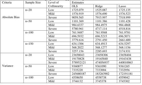
Table 1: Average of estimates of parameters from the various criteria

Criteria Sample Size Level of Collinearity

Estimates

OLS Ridge Lasso

Absolute Bias

n=20 Low 1725.079 1525.087 1725.135

Mild 1576.919 1576.690 1576.523

Severe 9059.565 7915.997 7518.999

n=50 Low 1101.369 1101.386 1101.428

Mild 984.6337 984.4975 984.4868

Severe 5780.961 4717.114 4518.816

n=100 Low 761.9487 761.9568 761.9781

Mild 696.5932 696.5215 696.5071

Severe 3779.616 2791.450 2661.600

n=150 Low 634.1306 634.4913 634.5297

Mild 568.2022 568.1277 568.1156

Severe 3257.156 2285.693 2174.931

Variance

n=20 Low 23658043 23658306 23658404

Mild 19170828 19165840 19163438

Severe 578952121 474056937 440010063

n=50 Low 9360877 9361090 9361265

Mild 7335220 7333004 7332956

Severe 245680187 183263902 172191181

n=100 Low 4558650 4558738 4559042

[Badawaire* 5(2): February, 2018] ISSN 2349-4506

Impact Factor: 3.799

G

lobal

J

ournal of

E

ngineering

S

cience and

R

esearch

M

anagement

Severe 10278835 65479536 60841448

n=150 Low 3104887 3105005 3105297

Mild 2445341 2444641 2444581

Severe 75565712 44194248 40810412

RMSE

n=20 Low 2195.891 2195.900 2195.992

Mild 1988.571 1988.280 1988.116

Severe 11242.091 10174.941 9803.312

n=50 Low 1381.303 1381.324 1381.397

Mild 1230.100 1229.893 1229.873

Severe 7318.058 6323.498 6129.644

n=100 Low 962.1928 962.1981 962.2022

Mild 878.6355 878.4742 878.4466

Severe 4736.598 3782.861 3646.823

n=150 Low 794.1306 794.1492 794.2007

Mild 710.1862 710.0991 710.0867

Severe 4060.467 3107.574 2986.482

From table 1 above, it can be observed that the absolute biases, variances and root mean square errors of all the estimators decreases as the sample size increases.

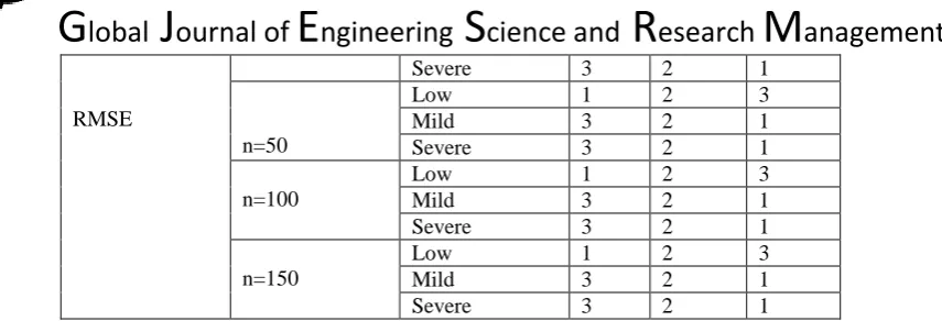
Results in table 1 for the estimators are ranked for each criterion and at each sample size, from the one with lowest average value as 1, to the one with highest average value as 3. The ranks are presented in table 2 below.

Table 2. Ranks of the Estimators Using Various Criteria

Criteria Sample Size Level of Collinearity

Estimators

OLS Ridge Lasso

Absolute Bias

n=20

Low 1 2 3

Mild 3 2 1

Severe 3 2 1

n=50

Low 1 2 3

Mild 3 2 1

Severe 3 2 1

n=100

Low 1 2 3

Mild 3 2 1

Severe 3 2 1

n=150

Low 1 2 3

Mild 3 2 1

Severe 3 2 1

Variance

n=20

Low 1 2 3

Mild 3 2 1

Severe 3 2 1

n=50

Low 1 2 3

Mild 3 2 1

Severe 3 2 1

n=100

Low 1 2 3

Mild 3 2 1

Severe 3 2 1

n=150

Low 1 2 3

Mild 3 2 1

Severe 3 2 1

n=20

Low 1 2 3

[Badawaire* 5(2): February, 2018] ISSN 2349-4506

Impact Factor: 3.799

G

lobal

J

ournal of

E

ngineering

S

cience and

R

esearch

M

anagement

RMSE

Severe 3 2 1

n=50

Low 1 2 3

Mild 3 2 1

Severe 3 2 1

n=100

Low 1 2 3

Mild 3 2 1

Severe 3 2 1

n=150

Low 1 2 3

Mild 3 2 1

Severe 3 2 1

From table 2 above it could be deduced that, when the collinearity level between the predictors is low, at all the sample sizes considered, OLS has the smallest ranks in all the three criteria for assessment. It can as well be observed that when the collinearity level between the predictors is mild or severe, at all the sample sizes considered, Lasso estimator consistently has the smallest ranks in all the three criteria.

From table 2 above, the table of preference of these estimators at varying degree of multicollinearity and at different sample size is formed, with the estimator having rank 1 as the most preferred estimator.

Table 3: Preference of the estimators

Criteria Sample Size Collinearity Level Most Preferred Estimator

Absolute Bias

n=20

Low OLS

Mild Lasso

Severe Lasso

n=50

Low OLS

Mild Lasso

Severe Lasso

n=100

Low OLS

Mild Lasso

Severe Lasso

n=150

Low OLS

Mild Lasso

Severe Lasso

Variance

n=20

Low OLS

Mild Lasso

Severe Lasso

n=50

Low OLS

Mild Lasso

Severe Lasso

n=100

Low OLS

Mild Lasso

Severe Lasso

n=150

Low OLS

Mild Lasso

Severe Lasso

n=20

Low OLS

Mild Lasso

Severe Lasso

n=50

Low OLS

[Badawaire* 5(2): February, 2018] ISSN 2349-4506

Impact Factor: 3.799

G

lobal

J

ournal of

E

ngineering

S

cience and

R

esearch

M

anagement

From table 3 above, it can be posited that OLS is the most preferred estimator at all the four sample sizes using both the criteria when the collinearity level is low, but when the collinearity level between the regressors is mild or severe, going by the three criteria and at all the four sample sizes, Lasso is the most preferred estimator.

CONCLUSION

In this study, the efficiency of four methods of parameter estimation when the assumption of ‘’no multicollinearity among the predictors considered in a model’’ is violated is investigated.Results from Monte Carlo experiments have shown that under low collinearity condition, irrespective of the sample size, OLS is the most efficient estimator.

Again when the collinearity condition between the predictors is mild or severe, irrespective of the sample size, Lasso is the most efficient estimator.

RMSE Severe Lasso

n=100

Low OLS

Mild Lasso

Severe Lasso

n=150

Low OLS

Mild Lasso

[Badawaire* 5(2): February, 2018] ISSN 2349-4506

Impact Factor: 3.799

G

lobal

J

ournal of

E

ngineering

S

cience and

R

esearch

M

anagement

REFERENCES

1. Alin, A. (2010), Multicollinearity. Willey Interdisciplinary Reviews: Computational Statistics, 2, 370-374.

2. Belsley, D. A. (1991), Conditioning Diagnostics Collinearity and Week Data in Regression. New York: Wiley- Interscience.

3. Fu, W. & Knight, K. (2000), Asymptotic for Lasso-type estimators. Ann. Stat., 28, 1356-1378.

4. Grewal, R., Cote, J. A., & Baumgartner, H. (2004),Multicollinearity and Measurement Error in Structural Equation Models: Implications for Theory Testing. Marketing Science, 23, 519-529.

5. Gujarati, D. N. (2004), Basic Econometrics, (4th _{Ed.).The McGraw-Hill Companies.NewYork.}

6. Hoerl, A. E., & Kennard, R. W. (1970), Ridge Regression: Biased Estimation for Nonorthogonal Problems. Technometrics, 12, 55-67.

7. Li, Y. F., Xie, M., &Goh, T. N. (2010), Adaptive Ridge Regression System for Software Cos Estimation On Multi-Collinear Datasets. Jounal of Systems and Software, 83, 2332-2343.

8. Lounici, K. (2008), Sub-norm convergence rate and sign concentration property of Lasso and Dantzig estimators.Electronic Journal of Statistics, 2.

9. Murray, M. P. (2006), Econometrics A Modern Introduction. Boston: Addison-Wesley. 10. Stewart, G. W. (1987),Collinearity and Least Squares Regression. Statistical Science, 2, 68-84.

11. Stock, J. H., & Watson, M. W. (2007), Introduction toEconometrics. (D. Clinton, Ed., 2nd_ed.). International Edition: Pearson Education.

12. Wan, A. T. K. (2002),On Generalized Ridge Regression Estimation Under Collinearity and Balanced Loss. Applied Mathematics and Computation, 129, 455-467.