Improving the Accuracy of the Solutions of
Riccati Equations
A. R. Vahidia∗, M. Didgarb
(a)Department of Mathematics, Shahr-e-Rey Branch, Islamic Azad University, Tehran, Iran
(b)Department of Mathematics, Science and Research Branch, Islamic Azad University, Tehran, Iran Received 4 July 2011; revised 9 December 2011, accepted 12 December 2011.
———————————————————————————————-Abstract
In this paper, we present an improved method for solving Riccati equations. This mod-ification is based on the previous scheme to obtain the approximate solution of Riccati equations [B.Q. Tang and X.F. Li, A new method for determining the solution of Ric-cati differential equations, Appl. Math. Comput. 194 (2007) 431-440]. Some numerical illustrations are given to show the effectiveness and high accuracy of the proposed modi-fication.
Keywords: Riccati equation; Volterra integral equation; Taylor expansion.
————————————————————————————————–
1
Introduction
Consider the Riccati equation of the form
w′(x) =p(x) +q(x)w(x) +r(x)w2(x), r(x)̸= 0. (1.1) Nonlinear differential equations are essential tool for modeling many physical situations such as: spring-mass systems, resistor-capacitor-inductance circuits, bending of beams, chemical reactions, pendulums, the motion of rotating mass around another body, and so forth. This kind of equations have also demonstrated their usefulness in ecology and economics. Thus, methods of solving these equations are of great importance to engineers and scientists [11].
Since the beginning of the 1980s, the Adomian decomposition method (ADM) [4, 5] and the homotopy perturbation method (HPM) [9, 10] have been applied to a wide class of functional equations. Bulut and Evans applied the ADM to obtain the approximate solution of the Riccati equation [7]. El-Tawil et al used the multistage Adomian’s decom-position method which can be used to obtain the solution for the whole time horizon [8].
∗Corresponding author. Email address: [email protected]
In this method, the time interval is divided into n equal subintervals and the method is applied once to each subinterval. Abbasbandy solved the Riccati equation by the homo-topy perturbation method [1], the iterated He’s homohomo-topy perturbation method [2] and He’s variational iteration method [3] while these methods have acceptable accuracy in the whole time horizon, they have some disadvantages in the solution intervals. For example, there is not any clear-cut criterion for partitioning the interval into an appropriate number of subintervals. In addition, the iterated HPM needs solving a linear functional equation in each iteration, which sometimes is very difficult and even impossible.
Bao-Qing Tang and Xian-Fang Li in [6] proposed a novel method for solving Riccati equations. Their method is based on converting the Riccati equation to a second-order ordinary differential equation, then to a Volterra integral equation. Finally the Taylor expansion is used to obtain the approximate solution. Therefore the accuracy of the approximate solutions depends on the order of the Taylor expansion. An advantage of this method is that it can be used for solving Riccati equations with both constant and variable coefficients.
By comparing the approximate solutions of above mentioned method with other meth-ods and evaluating errors, one can get that although the accuracy of the approximate solutions of the proposed method is not very high, the method leads not to be divergent. Furthermore, the graphs of the approximate solutions follow the graph of the exact solu-tion, which represents an advantage of new approach in comparison with the ADM and the HPM for solving Riccati equations. This method approximates the exact solution in the whole of interval contrary to other methods that approximate the exact solution in a small interval.
In this paper, we modify the proposed method and improve the accuracy of the approx-imate solutions, remarkably. In particular, at the beginning of the interval, the accuracy is very high and the graphs of the approximate solutions follow the exact solution nicely. This paper is arranged as follows. In Section 2, we introduce the structure of the proposed method in [6]. In Section 3, the modified method is presented. We indicate the effectiveness of the modified technique through several examples in Section 4. In Section 5, findings are summarized.
2
Mathematical formulation
In this section, we explain the method proposed by Bao-Qing Tang and Xian-Fang Li for solving the Riccati equation [6]. In this method, Eq. (1) will be transformed into an equivalent Volterra integral equation [6]. To achieve this end, with the following change of variable
w(x) =− y
′(x)
r(x)y(x), (2.2)
we transform Eq. (1) into a second-order homogeneous ordinary differential equation as follows
r(x)y′′−[r′(x) +r(x)q(x)]y′+p(x)r2(x)y= 0. (2.3) In view of transformation (2), we can easily deduce the integral form of the solution as
y(x) =Cexp(− ∫ x
x0
whereCis an arbitrary constant. In what follows, without loss of generality, we letC= 1 and obtain the initial conditions as y(x0) = 1 and y′(x0) =−w(x0)r(x0).
By integrating both sides of Eq. (2.3) twice with respect to xfrom x0 toxsubject to initial conditions, we obtain a Vloterra integral equation as follows
y(x) + ∫ x
x0
k(x, t)y(t)dt=f(x), (2.5)
where
k(x, t) = (x−t)[p(t)r(t) +q′(t) + (r
′(t)
r(t))
′]−[q(t) +r′(t)
r(t)], (2.6)
f(x) = 1−w(x0)r(x0)x−[q(x0) +
r′(x0)
r(x0)]x. (2.7)
Now, using the method suggested in [12], we employ the Taylor expansion for the unknown functiony(t) at x
y(t)≈y(x) +y′(x)(t−x) +...+ 1
n!y
(n)(x)(t−x)n. (2.8)
Substituting (2.8) for y(t) in the integrand into (2.5) leads to
y(x) + n ∑
j=0 (−1)j
j! y (j)(x)
∫ x
x0
k(x, t)(x−t)jdt=f(x). (2.9)
Note that a notation y(0) = y(x) is adopted. In Eq. (2.9) y(j)(x), for j = 0, . . . , n are unknown functions. In order to obtain these unknown functions, we consider the above equation as a linear equation for y(x) and its derivatives up to n. Consequently, other
n independent linear equations fory(x) and their derivatives up to n are needed. These equations can be obtained by the integration of both sides of Eq. (2.5)ntimes as follows
∫ x
x0
(x−t)i−1y(t)dt+ ∫ x
x0 ∫ x
t
(x−s)i−1k(s, t)y(t)dsdt=f(i)(x), 1≤i≤n, (2.10)
where
f(i)(x) = ∫ x
x0
(x−t)i−1f(t)dt. (2.11)
Inserting (2.8) for y(t) into Eq. (2.10) leads to
∫ x
x0
(x−t)i−1 n
∑
j=0
(−1)j j! y
(j)(x)(x−t)jdt+
∫ x
x0 ki(x, t)
n
∑
j=0
(−1)j j! y
(j)(x)(x−t)jdt=f
(i)(x),(2.12) where
ki(x, t) = ∫ x
t
Hence, Eqs. (2.9) and (2.12) form a system of linear equations for the unknowns y(x) and its derivatives up to n.
Introducing
C(x) =
c00(x) c01(x) . . . c0n(x)
c10(x) c11(x) . . . c1n(x) ..
. ... . .. ...
cn0(x) cn1(x) . . . cnn(x)
, (2.14)
F(x) =
f(x)
f(1)(x) .. .
f(n)(x)
, Y(x) =
y(x)
y′(x) .. .
y(n)(x)
, (2.15)
the above system composed of Eqs. (2.9) and (2.12) can be rewritten as
C(x)Y(x) =F(x), (2.16)
where in (2.14), the first row refers to coefficients of y(j)(x) in Eq. (2.9) forj = 0, . . . , n
and the other rows refer to coefficients ofy(j)(x) in Eq. (2.12) forj = 0, . . . , n. Applying of Cramer’s rule to the resulting system yields an approximate solution of Eq. (2.3). We note that not only y(x) but also y(j)(x), for j = 1, . . . , n, are determined by solving the resulting system. Accordingly, in view of (2.2), a desired solutionw(x) can be represented by the nth-order approximations
wn(x) =−
det(C1(x))
r(x)det(C0(x))
, (2.17)
where
C0(x) =
f(x) c01(x) . . . c0n(x)
f(1)(x) c11(x) . . . c1n(x) ..
. ... . .. ...
f(n)(x) cn1(x) . . . cnn(x)
, (2.18)
C1(x) =
c00(x) f(x) . . . c0n(x)
c10(x) f(1)(x) . . . c1n(x) ..
. ... . .. ...
cn0(x) f(n)(x) . . . cnn(x)
, (2.19)
3
Modified method
In the previous section, in view of transformation (2), we obtained an approximate solution forw(x) as
wn(x) =−
yn′(x)
r(x)yn(x)
=− det(C1(x))
r(x)det(C0(x))
, (3.20)
where
yn(x) =
det(C0(x))
det(C(x)), (3.21)
yn′(x) = det(C1(x))
det(C(x)), (3.22)
and bothyn(x) andyn′(x) are calculated by Cramer’s rule.
In this section, we propose a modified method to evaluatey′(x) which doesn’t need to use Cramer’s rule again.
Now, in order to modify the method, we consider the Maclaurin expansion of y(x) obtained in section 2 and name it yM(x). In what follows, we useyM(x) instead of y(x). Next we need to estimatey′(x). To reach this end, we differentiateyM(x). Consequently, a desired solutionw(x) can be represented by thenth-order approximations
wn(x) =−
yM′ (x)
r(x)yM(x)
. (3.23)
By applying the modified method, we can improve the accuracy, remarkably. In particular, the accuracy is very high at the beginning of the interval, .
4
Test examples
In this section, we solve three test examples to demonstrate the effectiveness of our modification. Absolute errors at equidistant points are shown in tables, comparing two methods introduced in Section 3 and in [6]. All results are calculated by using the MATH-EMATICA software package.
Example 4.1. Consider the following Riccati equation
w′(x) = 1 + 2w(x)−w2(x), (4.24)
with the initial condition w(0) = 0, which has the exact solution
w(x) = 1 +√2tanh[√2x+1 2log(
√
2−1
√
2 + 1)]. (4.25)
Using the proposed method, we can evaluate the approximate solutions of Eq. (4.24). First, by applying the introduced method in section (2) we obtainy(x). For example, whenn= 2 in the Taylor expansion, one can obtain y(x) as follows
y(x) = 12(−600 + 720x−630x
2+ 200x3−31x4+ 2x5)
Then by calculating the Maclaurin expansion of y(x) up to order 7, we get
yM(x) = 1 +
x2 2 +
x3 3 +
5x4 24 +
x5 10 +
157x6 3600 +
211x7
9000 . (4.27) Consequently, in view of (3.23) and by calculating y′M(x), we obtain
w2(x) =
2x(9000 + 9000x+ 7500x2+ 4500x3+ 2355x4+ 1477x5)
18000 + 9000x2+ 6000x3+ 3750x4+ 1800x5+ 785x6+ 422x7. (4.28) Other nth-order approximationswn(x) for n= 3,4, . . . are similarly evaluated, which are
not shown here. To continue, we compare the absolute errors of the approximate solutions, taking n= 5,6 with two methods presented in [6] and this paper.
Absolute errors at twenty equidistant points in the interval[0,4]are shown in Tables 1 and 2. In the following Tables, E1 and E2 show the absolute errors of methods presented in [6] and in this paper taking n = 5,6, respectively. For n = 5 and n = 6, we have calculated the Maclaurin expansion of y(x) up to order 14 and 16, respectively.
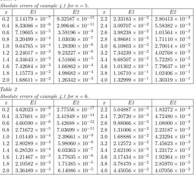
Table 1
Absolute errors of example 4.1 forn= 5.
x E1 E2 x E1 E2
0.2 2.14179×10⁻⁷ 9.32587×10⁻¹⁵ 2.2 2.33183×10⁻² 2.80413×10⁻³ 0.4 8.33086×10⁻⁶ 2.99646×10⁻¹¹ 2.4 3.09707×10⁻² 5.58382×10⁻³ 0.6 7.19605×10⁻⁵ 3.59196×10⁻⁹ 2.6 3.98238×10⁻² 1.01564×10⁻² 0.8 3.20499×10⁻⁴ 1.03036×10⁻⁷ 2.8 4.98681×10⁻² 1.71110×10⁻² 1.0 9.64765×10⁻⁴ 1.28390×10⁻⁶ 3.0 6.10803×10⁻² 2.70014×10⁻² 1.2 2.24017×10⁻³ 9.23227×10⁻⁶ 3.2 7.34239×10⁻² 4.02768×10⁻² 1.4 4.34643×10⁻³ 4.51666×10⁻⁵ 3.4 8.68507×10⁻² 5.72285×10⁻² 1.6 7.42684×10⁻³ 1.66862×10⁻⁴ 3.6 1.01302×10⁻¹ 7.79637×10⁻² 1.8 1.15773×10⁻² 4.98682×10⁻⁴ 3.8 1.16710×10⁻¹ 1.02406×10⁻¹ 2.0 1.68611×10⁻² 1.26342×10⁻³ 4.0 1.32999×10⁻¹ 1.30319×10⁻¹ Table 2
Absolute errors of example 4.1 forn= 6.
x E1 E2 x E1 E2
0.2 4.62023×10⁻⁹ 2.77556×10⁻¹⁷ 2.2 5.04887×10⁻³ 1.83272×10⁻⁴ 0.4 3.57601×10⁻⁷ 3.41949×10⁻¹⁴ 2.4 7.20720×10⁻³ 4.72480×10⁻⁴ 0.6 4.60590×10⁻⁶ 5.42688×10⁻¹² 2.6 9.88066×10⁻³ 1.08000×10⁻³ 0.8 2.71672×10⁻⁵ 7.03699×10⁻¹¹ 2.8 1.31006×10⁻² 2.23187×10⁻³ 1.0 1.01449×10⁻⁴ 2.39661×10⁻⁹ 3.0 1.68886×10⁻² 4.23294×10⁻³ 1.2 2.80289×10⁻⁴ 5.98060×10⁻⁸ 3.2 2.12572×10⁻² 7.45623×10⁻³ 1.4 6.28520×10⁻⁴ 6.03363×10⁻⁷ 3.4 2.62100×10⁻² 1.23172×10⁻² 1.6 1.21467×10⁻³ 3.77635×10⁻⁶ 3.6 3.17434×10⁻² 1.92364×10⁻² 1.8 2.10582×10⁻³ 1.71385×10⁻⁵ 3.8 3.78470×10⁻² 2.85970×10⁻² 2.0 3.36489×10⁻³ 6.14086×10⁻⁵ 4.0 4.45056×10⁻² 4.07056×10⁻²
Tables 1 and 2 indicate the effectiveness of the modified method. In particular, we ob-serve that the accuracy is very high at the beginning of the interval.
1 2 3 4 0.5
1.0 1.5 2.0
Fig. 1. The exact solution (solid) versus the approximate solution (bolded dash). Example 4.2. Consider the following Riccati equation
w′(x) = 1 +x2−w2(x), (4.29)
subject tow(0) =C whereC is a constant. The exact solution of the above Riccati equation is
w(x) =x+ Ce
−x2
1 +C∫0xe−t2
dt. (4.30)
In the case ofC= 1, using our proposed method, we can obtain the approximate solution of the Riccati equation. First, for n= 4,6, we obtain y(x) and then calculate the Maclaurin expansion of y(x) up to order 20, 28 corresponding to n= 4,6, respectively.
Absolute errors at twenty equidistant points in the interval[0,4]are shown in Tables 3 and 4. In the following Tables, E1 and E2 show the absolute errors of methods presented in [6] and this paper taking n= 4,6, respectively.
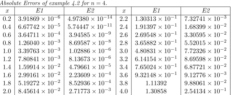
Table 3
Absolute Errors of example 4.2 for n= 4.
x E1 E2 x E1 E2
Table 4
Absolute Errors of example 4.2 for n= 6.
x E1 E2 x E1 E2
0.2 1.75971×10⁻⁹ 0 2.2 1.20948×10⁻² 1.80898×10⁻⁶ 0.4 1.38446×10⁻⁷ 6.66134×10⁻¹⁶ 2.4 2.13966×10⁻² 1.80141×10⁻⁵ 0.6 1.90408×10⁻⁶ 1.62981×10⁻¹³ 2.6 3.57479×10⁻² 1.29406×10⁻⁴ 0.8 1.27184×10⁻⁵ 1.02709×10⁻¹¹ 2.8 5.68025×10⁻² 5.34823×10⁻⁴ 1.0 5.68465×10⁻⁵ 2.53517×10⁻¹⁰ 3.0 8.63430×10⁻² 1.64884×10⁻³ 1.2 1.96039×10⁻⁴ 3.39761×10⁻⁹ 3.2 1.26173×10⁻¹ 4.04101×10⁻³ 1.4 5.62481×10⁻⁴ 2.91749×10⁻⁸ 3.4 1.77999×10⁻¹ 7.97472×10⁻³ 1.6 1.40404×10⁻³ 1.74448×10⁻⁷ 3.6 2.43309×10⁻¹ 1.23386×10⁻² 1.8 3.13752×10⁻³ 7.41881×10⁻⁷ 3.8 3.23282×10⁻¹ 1.32183×10⁻² 2.0 6.40115×10⁻³ 2.07300×10⁻⁶ 4.0 4.18716×10⁻¹ 3.04960×10⁻³
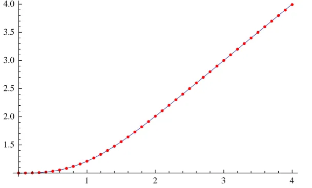
Moreover, Fig. 2 shows the exact solution and the approximate solution, obtained from the proposed method in this paper for n = 6. It illustrates that our new approach has a good convergence through the applicable domain.
1 2 3 4
1.5 2.0 2.5 3.0 3.5 4.0
Fig. 2. he exact solution (solid) versus the approximate solution (bolded dash). Example 4.3. Consider the following Riccati equation
w′(x) = 1 +w2(x), (4.31)
with the initial condition w(0) = 0 which has the exact solution w(x) = tan(x). In this example, we study cases n= 3,6. Forn= 3, we evaluate the Maclaurin expansion ofy(x) up to order 8 and when n= 6 we calculate the Maclaurin expansion of y(x) up to order 14.
Table 5
Absolute errors of example 4.3 forn= 3.
x E1 E2
0.1 4.77556×10⁻⁶ 5.67699×10⁻¹³ 0.3 1.31998×10⁻⁴ 1.25556×10⁻⁹ 0.5 6.42351×10⁻⁴ 4.59033×10⁻⁸ 0.7 1.91631×10⁻³ 5.02099×10⁻⁷ 0.9 4.65106×10⁻³ 3.08180×10⁻⁶ 1.1 1.05496×10⁻² 1.36974×10⁻⁵ 1.3 2.60423×10⁻² 5.27239×10⁻⁵ 1.5 1.29891×10⁻¹ 4.07727×10⁻⁴ Table 6
Absolute errors of example 4.3 forn= 6.
x E1 E2
0.1 4.64490×10⁻¹⁴ 0
0.3 1.05268×10⁻¹⁰ 5.55112×10⁻¹⁷ 0.5 4.05170×10⁻⁹ 1.11022×10⁻¹⁶ 0.7 4.82526×10⁻⁸ 4.77396×10⁻¹⁵ 0.9 3.37725×10⁻⁷ 2.70228×10⁻¹³ 1.1 1.83698×10⁻⁶ 7.95874×10⁻¹² 1.3 9.71748×10⁻⁶ 1.88015×10⁻¹⁰ 1.5 9.63926×10⁻⁵ 1.09076×10⁻⁸
Moreover, Fig. 3 shows the exact solution and the approximate solution obtained from the proposed method in this paper for n = 3. It illustrates that our new approach has a good convergence through the applicable domain.
0.2 0.4 0.6 0.8 1.0 1.2 1.4
1 2 3 4 5 6
Fig. 3. The exact solution (solid) versus the approximate solution (bolded dash).
5
Conclusion
equation could be approximately solved. In view of (2), we proposed a new method for calculating y′(x) and improved the accuracy of the approximate solutions.
References
[1] S. Abbasbandy, Homotopy perturbation method for quadratic Riccati differential equation and comparison with Adomian’s decomposition method, Appl. Math. Com-put. 172 (2006) 485-490.
[2] S. Abbasbandy, Iterated He’s homotopy perturbation method for quadratic Riccati differential equation, Appl. Math. Comput. 175 (2006) 581-589.
[3] S. Abbasbandy, A new application of He’s variational iteration method for quadratic Riccati differential equation by using Adomian’s polynomials, J. Comput. Appl. Math. 207 (2007) 59-63.
[4] G. Adomian, Nonlinear Stochastic Systems Theory and Applications to Physics, Kluwer Academic, Dordrecht, 1989.
[5] G. Adomian, Solving Frontier Problems of Physics: The Decomposition Method, Kluwer Academic, Dordrecht, 1994.
[6] Bao-Qing Tang, Xian-Fang Li, A new method for determining the solution of Riccati differential equations, Appl. Math. Comput. 194 (2007) 431-440.
[7] H. Bulut, D. J. Evans, On the solution of the Riccati equation by the decomposition method, Int. J. Comput. Math. 79 (2002) 103-109.
[8] M. A. El-Tawil, A. A. Bahnasawi, A. Abdel-Naby, Solving Riccati differential equation using Adomian’s decomposition method, Appl. Math. Comput. 157 (2004) 503-514.
[9] J. H. He, An approximate solution technique depending upon an artificial parameter, Commun. Nonlinear Sci. Simulat. 3 (2) (1998) 92-97.
[10] J. H. He, Homotopy perturbation technique, Comput. Methods App1. Mech. Engng. 178 (3-4) (1999) 257-262.
[11] W.T. Reid, Riccati Differential Equations, Academic Press, New York, 1972.