Solving singular integral equations by using orthogonal polynomials

(1)

Solving singular integral equations by using orthogonal polynomials

Samad Ahdiaghdam

Department of Mathematics, Marand Branch, Islamic Azad University, Marand, Iran.

Abstract In this paper, a special technique is studied by using the orthogonal Chebyshev polynomials to get approximate solutions for singular and hyper-singular integral equations of the ﬁrst kind. A singular integral equation is converted to a system of algebraic equations based on using special properties of Chebyshev series. The error bounds are also stated for the regular part of approximate solution of singular integral equations. The eﬃciency of the method is illustrated through some examples.

Keywords. Singular integral equations, Chebyshev systems, Approximate quadratures. 2010 Mathematics Subject Classification. 45E05, 41A50, 41A55.

1. _Introduction

Let us consider a singular integral equation of the form ∫1

−1 ψ(t) (t−x)αdt+

∫ 1

−1

K(t, x)ψ(t)dt=f(x), −1< x <1, α∈N, (1.1)

where the functionsK(t, x) and f(x) are given real-valued H¨older continues functions and ψ(t) is the unknown function to be determined.

The first integral in (1.1) is known as the finite part integral, which was firstly introduced by J. Hadamard who generalized the Cauchy singular integral equations [11]. The singular-ities of Eq. (1.1) would be mentioned as Cauchy or Hadamard type forα= 1 andα > 1, respectively.

Equations of the form (1.1) arise in the study of obtaining solutions to mixed boundary value problems of mathematical physics and theoretical mechanics, particularly in the areas of elasticity, aerodynamics, and unsteady aerofoil theory [12].

The classical theoretical and numerical studies on the Eq. (1.1) in the caseα= 1 are given in [15] and [7] by Muskhelishivi and Goldberg, respectively. The recent studies on the Eq. (1.1) can be found in [5,8,9,10,14,17,18]. For example, Eshkuvatov and Long [5] presented new quadrature formulas to approximate the singular integrals of Cauchy type by utilizing linear spline interpolation, modified discrete vortex and product integration methods. But they only considered the caseK(t, x) = 0 andα= 1, i.e., the characteristic singular integral equation. Kashfi and Shahmorad [10] constructed an approximate solution for Eq. (1.1) in the caseα= 1 by using Chebyshev polynomials of the first and second kinds. Setia [17] developed a numerical method to solve various types of Cauchy singular integral equations by using Bernstein polynomials. Karczmarek et. al. [9] have approximated the solution of

Received: 3 December 2017 ; Accepted: 20 August 2018.

(2)

such Cauchy type singular integral equations by using Jacobi polynomials. Tsalamengas [18] derived quadrature rules for Cauchy and Hadamard type singular integrals of the form

I±(K, ψ, t) =

∫ 1

−1

ω(t)ψ(t)K(t, x)dt, ω(t) = (1−t2)±1/2,

from corresponding quadrature rules for logarithmic singular integrals.

For the caseα= 1 a convergence analysis of Galerkin and collocation methods for Eq. (1.1) has been given by Miel [14]. Zhang et. al. [19] discussed a pointwise superconvergence of the composite trapezoidal rule for Hadamard ﬁnite part integrals.

A special case of Eq. (1.1) is the famous characteristic singular integral equation

∫1

−1 ψ(t)

t−xdt=f(x), −1< x <1. (1.2)

For the H¨older continues f(x), the Eq. (1.2) has analytical solution in four diﬀerent forms given by

ψ(t) :=ωr(t)ϕr(t), r= 1,2,3,4, (1.3)

where

ϕr(t) =a0−

1 π2

∫ 1

−1

f(x) ωr(x)(x−t)

dx, −1< t <1, (1.4)

and

ωr(t) =

λr(t)

√

1−t2 , λr(t) =

      

1, r= 1, 1−t2, r= 2, 1 +t, r= 3, 1−t, r= 4,

(1.5)

(See [5,7,12,17]). In the caser= 1,a0 is an arbitrary constant, whereas in other cases we havea0 = 0. For ∫₋₁1 ψ(t)dt=Const.the uniqueness of solution is also guaranteed in the caser= 1. A necessary and suﬃcient condition for existence of solution in the caser= 2 is given by

∫ 1

−1 f(x)

ω2(x)dx= 0.

An application of Eq. (1.2) were given in [1] by reducing a system of dual integral equations to Cauchy type singular integral equations.

Letα= 1. By using (1.3)-(1.4) and a simple manipulation, Eq. (1.1) is converted to the linear Fredholm integral equation

ϕr(t) + ∫ 1

−1

ωr(τ)Kr(t, τ)ϕr(τ)dτ =Fr(t), −1< t <1, r= 1,2,3,4, (1.6)

where _

   

Fr(t) =−_π12 ∫1

−1

f(x)

ωr(x)(x−t)dx,

Kr(t, τ) =−_π12 ∫1

−1

K(τ,x)

ωr(x)(x−t)dx.

Since K(t, x) is H¨older continuous, then Kr(t, τ) is generally integrable and one may

proceed to solve Eq. (1.6) numerically [7].

(3)

2. Approximate solution of Cauchy integral equation

The Chebyshev polynomial is like a fine jewel that reveals different characteristics un-der illumination from varying positions [16]. There are many applications of Chebyshev polynomials, specially in solving differential and integral equations. After presenting a brief introduction about these polynomials, we apply them to construct approximate solution for Eq. (1.1).

An inﬁnite series of the form ∞

∑

i=0

aiPr,i(t), r= 1,2,3,4,

is called a Chebyshev series. Fort= cos(θ), we have

Pr,j(t) =                   

Tj(t) = cos(jθ), r= 1,

Uj(t) = sin ((j+ 1)θ)/sin(θ), r= 2,

Vj(t) = cos (

(j+1₂)θ)/cos(θ₂), r= 3,

Wj(t) = sin (

(j+1₂)θ)/sin(θ₂), r= 4,

(2.1)

which are known as the ﬁrst, second, third and fourth kind Chebyshev polynomial, respec-tively.

The functionsPr,j satisfy the orthogonality properties

µrij:=

1

π < Pr,i, Pr,j>r=

          

0, i̸=j,

1, i=j= 0, r= 1, 1/2, i=j̸= 0, r= 1, 1/2, i=j, r= 2, 1, i=j, r= 3,4,

(2.2)

with respect to the inner product

< f, g >r= ∫ 1

−1

ωr(t)f(t)g(t)dt ,

whereωr(t), the weight function, is determined from (1.5).

Now, we recall the following theorem from [13].

Theorem 2.1. As a Cauchy principle value integral, we have

Qr,i(x) :=

1 π

∫ 1

−1

ωr(t)Pr,i(t)

t−x dt =

      

Ui−1(x), r= 1,

−Ti+1(x), r= 2,

Wi(x), r= 3,

−Vi(x), r= 4.

(2.3)

For every integrable functionf onI= [−1,1], there is a Chebyshev expansion

f(x) := ∞

∑

j=0

cjPr,j(x), r= 1,2,3,4,

associated with the Chebyshev polynomial of kindr, where

cj=

1 π µr

jj ∫1

−1

(4)

Now, we are in a position to use the Chebyshev polynomials to construct an approximate solution to the Eq. (1.1) in the caseα= 1. To do this, we set

ϕr(t) :=

∞

∑

i=0

aiPr,i(t), r= 1,2,3,4, (2.4)

in (1.3) and

K(t, x)≃κ(t, x) :=

M ∑

j=0

bj(x)Pr,j(t), r= 1,2,3,4, (2.5)

where the coeﬃcientsai,s are unknown, butbj(x),s are determined as

bj(x) =

1 π µr

jj ∫ 1

−1

ωr(t)κ(t, x)Pr,j(t)dt, j= 0,1, . . . , M,

which may be calculated approximately by using a Gauss-Chebyshev quadrature rule, i.e.,

bj(x)≃

4 ηr

M∑+1

n=1

λr(τr,n)κ(τr,n, x)Pr,j(τr,n), j= 0,1, . . . , M,

in which{τr,n}M_n₌₁+1are the roots ofPr,M+1(t), i.e.,

τr,n= {

cos ((2n−1)π/ηr), r= 1,3,

cos (2nπ/ηr), r= 2,4, (2.6)

for

ηr=   

2M+ 2, r= 1, 2M+ 4, r= 2, 2M+ 3, r= 3,4.

Substituting from (1.3) and (2.4)-(2.5) into Eq. (1.1) forα= 1 and using (2.2)-(2.3), gives the equations

∞

∑

i=σ

aiQr,i(x) + M ∑

i=0

µriiaibi(x) =F(x), σ= {

1, r= 1,

0, r= 2,3,4, (2.7)

where F(x) = f(x)/π. In what follows, we show that each of these equations leads to a system of linear algebraic equations in the casesr= 1,2,3,4.

Case 1.Forr= 1, the relations (2.4)-(2.5) take the forms

ϕ1(t) :=∑∞_i₌₀aiTi(t), and κ(t, x) := ∑M

j=0

′

bj(x)Tj(t),

where∑′ denotes that the ﬁrst term in the summation is halved. Therefore, Eq. (2.7) can be rewritten as

∞

∑

i=1

aiUi−1(x) +1 2

M ∑

i=0

aibi(x) =F(x). (2.8)

Let the functionsF(x) andbi(x) be integrable with respect to the weight functionω2(x) on

[−1, 1], then they can be expanded as

  

bi(x)≃ ∑M

j=0BijUj(x), i= 0,1, . . . , M,

F(x)≃∑M_j₌₀cjUj(x),

(5)

where fori, j= 0,1, . . . , M,the coeﬃcients     

Bij≃_π2 ∫1

−1 √

1−x2_b

i(x)Uj(x)dx≃ _π42 ∫1

−1

∫1 −1

√

1−x2

1−t2K(t, x)Ti(t)Uj(x)dtdx,

cj≃ _π22 ∫1

−1 √

1−x2_f(x)U

j(x)dx,

can be approximately computed by

    

Bij≃₍_M₊₁₎₍4_M₊₂₎ ∑M+1

m=1

∑M+1

n=1 (1−τ 2

2,m)K(τ1,n, τ2,m)Ti(τ1,n)Uj(τ2,m),

cj≃ _π₍_M2₊₂₎ ∑M+1

m=1(1−τ 2

2,m)f(τ2,m)Uj(τ2,m),

whereτr,nis given by (2.6). Using (2.9) in (2.8) yields

∞

∑

j=0

aj+1Uj(x) +

1 2 M ∑ j=0 M ∑ i=0

BijaiUj(x) = M ∑

j=0

cjUj(x),

which is reduced to the linear system of algebraic equations

aj+1+ 1 2

M ∑

i=0

Bijai=cj, j= 0,1, . . . , M, (2.10)

along with aj+1 = 0 for j > M, by using the orthogonality property (2.2) for r = 2. By solving the under-determined system (2.10) for coeﬃcients{aj}M_j₌₀+1we obtain inﬁnitely

many approximations forϕ1(t) asφ1(t) =∑M_i₌₀+1aiTi(t), which results (using (1.3)) inﬁnitely

many approximate solutions for (1.1) as

ψ(t) =ω1(t)ϕ1(t)≃ω1(t)φ1(t) =√ 1 1−t2

M∑+1

i=0

aiTi(t). (2.11)

Case 2.Forr= 2, we set

ϕ2(t) :=∑∞_i₌₀aiUi(t) and κ(t, x) := ∑M

j=0 bj(x)Uj(t),

then the relation (2.7) takes the form

−

M ∑

i=0

aiTi+1(x) +

1 2

M ∑

i=0

aibi(x) =F(x). (2.12)

Using the expansions

    

bi(x)≃ ∑M

j=0

′

BijTj(x), i= 1,2, . . . , M,

F(x)≃∑M_j₌₀′cjTj(x),

in Eq. (2.12), returns the over-determined linear algebraic system

   1 2 ∑M

i=0Bijai=cj, j= 0,

−aj−1+1₂ ∑M

i=0Bijai=cj, j= 1,2, . . . , M,

(2.13)

along withaj−1= 0 forj > M,where 

   

Bij≃ ₍_M₊₁₎₍4_M₊₂₎ ∑M+1

m=1

∑M+1

n=1(1−τ 2

2,n)K(τ2,n, τ1,m)Tj(τ1,m)Ui(τ2,n),

cj≃_π₍_M2₊₁₎ ∑M+1

(6)

Then, the functionψ(t) will be determined approximately from

ψ(t) =ω2(t)ϕ2(t)≃ω2(t)φ2(t) =√1−t2

M_∑−1

i=0

aiUi(t). (2.14)

Cases 3,4. Forr= 3,4, proceeding by the same way as we did in the casesr= 1,2, we get the linear systems

(−1)r+1aj+ M ∑

i=0

Bijai=cj, j= 0,1, . . . , M, r= 3,4 (2.15)

along withaj= 0 forj > M, which lead to the approximate solutions

ψ(t) =ωr(t)ϕr(t)≃ωr(t)φr(t) =        √ 1+t

1−t ∑M

i=0aiVi(t), r= 3,

√

1−t

1+t ∑M

i=0aiWi(t), r= 4.

(2.16)

3. Hadamard integral equation

Existence of the solution for the hyper-singular integral equations of the ﬁrst kind inves-tigated in the spacial caseα=r= 2, by Chen and Zhou [3].

To ﬁnd an approximate solution of Eq. (1.1) forα >1 in the casesr= 1,2,3,4, we ﬁrst notice that _∫

1 −1

ψ(t) (t−x)n+1dt=

1 n! dn dxn ∫ 1 −1 ψ(t)

t−xdt, n∈N.

Then, we substitute from (1.3) and (2.4)-(2.5) into Eq. (1.1) and use (2.2)-(2.3), to get

1 (α−1)!

dα−1 dxα−1

∞

∑

i=σ

aiQr,i(x) + M ∑

i=0

µriiaibi(x) =F(x), (3.1)

where

σ=

{

1, r= 1, 0, r= 2,3,4.

The next step is to convert Eq. (3.1) to the corresponding algebraic system. To do this, we ﬁrstly state the following lemma.

Lemma 3.1. Form≥1, we have

d

dxPr,m(x) =

                    

mUm−1(x), r= 1,

∑[m−1₂ ]

k=0 2(m−2k)Um−2k−1(x), r= 2,

∑m−1

k=0(−1)

k_2(m₋_k)U

m−k−1(x), r= 3,

∑m−1

k=0 2(m−k)Um−k−1(x), r= 4,

(3.2)

wherePr,m(x)is given by (2.1), andUj(x)is the Chebyshev polynomial of the second kind.

Proof. Forr= 1, it directly follows from (2.1)

d

dxTm(x) = d

dxcosmθ=

d dθcosmθ

dx dθ

=msinmθ

(7)

Forr= 2,3,4, the lemma is proved by induction. Here the details of the proof is stated for r= 2.

Letm= 1. Then

d

dxU1(x) = d

dx2x= 2 = 2U0(x) = [m_∑₂−1]

k=0

2(m−2k)Um−2k−1(x),

that is, (3.2) is true form= 1. Let (3.2) is satisﬁed form=n, i.e.,

d

dxUn(x) = [n_∑−1₂ ]

k=0

2(n−2k)Un−2k−1(x).

Form=n+ 1, we prove

d

dxUn+1(x) = [n

2] ∑

k=0

2(n−2k+ 1)Un−2k(x).

To do this, we use the relation

Un+1(x)−Un−1(x) = 2Tn+1(x),

from [13] and get

d

dxUn+1(x) = d

dx(2Tn+1(x) +Un−1(x)). Using (3.2) forr= 1 and the hypothesis of induction, results

d

dxUn+1(x) = 2(n+ 1)Un(x) + [n_∑−2₂ ]

k=0

2(n−2k−1)Un−2k−2(x)

= 2(n+ 1)Un(x) +

[n

2] ∑

j=1

2(n−2(j−1)−1)Un−2(j−1)−2(x)

= 2(n+ 1)Un(x) +

[n₂]

∑

j=1

2(n−2j+ 1)Un−2j(x)

= [n

2] ∑

j=0

2(n−2j+ 1)Un−2j(x),

which proves (3.2) forr= 2 andm=n+ 1. Forr= 3,4, use the relation

Vn+1(x) +Vn(x) =Wn+1(x)−Wn(x) = 2Tn+1(x).

Remark 3.2. Since the operator _dxdαα−−11 decreases degree of a polynomial α−1 times, we

(8)

Hence, forα= 2 by using lemma3.1the system of algebraic equations corresponding to Eqs. (3.1) take the following forms forj= 0,1, . . . , M,

                

2(j+ 1)∑[ M−j

2 ]+1

i=1 a2i+j+1₂ ∑M

i=0Bijai=cj, r= 1, −(j+ 1)aj+1₂

∑M

i=0Bijai=cj, r= 2,

2(j+ 1)∑M_i₌+1_j₊₁(−1)(r−1)(i−j)ai+ ∑M

i=0Bijai=cj, r= 3,4,

(3.3)

where forr= 1,2,3,4, we used (2.9).

4. Error bound

We recall the following deﬁnition and theorem from [10] describing an error bound for the approximate solution of Eq. (1.1) forα= 1 in the special caser= 1.

Definition 4.1. Letm≥0,0< ν≤1. We say that a functionf(x), x∈[−1,1] belongs to the classCm,ν if all the derivatives up to the orderminclusive exist and themthderivative belongs to the H¨older classH(ν):

|f(m)

(x)−f(m)(y)| ≤k|x−y|ν, ∀x, y∈[−1,1],

where the constantskandνare independent of choice of the pointsx, y.

Theorem 4.2. Suppose that the functionsf(x) andK(t, x) belong to the class Cm,ν _(the second function of both variables) for some m≥0,0< ν ≤1, and they are approximated by a ﬁnite Chebyshev series of orderM. Moreover, for suﬃciently large value of M, the homogeneous equation corresponding to (1.6) has only trivial solution. Then the system of linear equations (2.10) is nonsingular and

∥ϕ−φ∥∞≤Nln 2

(M)

Mm+ν, (4.1)

whereN is a constant independent ofM.

By considering the following relation between the ﬁrst and three other kinds of Chebyshev polynomials, the error bound (4.1) is conﬁrmed in the cases 2−4.

ωr(t)Pr,j(t) =ω1(t)           

1

2[Tj(t)−Tj+2(t)], r= 2, Tj(t) +Tj+1(t), r= 3,

Tj(t)−Tj+1(t), r= 4.

For a bounded and convex domain Ω⊂Rn_{, we have}_Cm+1_(Ω)_⊂_Cm,1_{(Ω) [}₂_{]. Therefore,} we deduce the following corollary.

Corollary 4.3. Letf(x)andK(t, x)are polynomials of degree less than or equal toM (the second function of both variables). Then f, K ∈ Cm,1 (m→ ∞) and so the right side of (4.1) tends to zero, i.e.,ϕ=φ.

(9)

Theorem 4.4. Let f ∈ Cr([−1,1]) and K ∈ Cr([−1,1]×[−1,1]). Then the Galerkin approximations

φ(t) =

M ∑

i=0 aiUi(t),

for the solution of

∫ 1

−1

√

1−t2 ϕ(t) (t−x)2dt+

∫ 1

−1

√

1−t2_{K(t, x)ϕ(t)dt}₌_f(x), ₋₁_{< x <}_1,

converge uniformly toϕ, and there exists n0∈Nsuch that

∥ϕ−φ∥∞=O(M−r+2),

for allM ≥max(n0, r+ 1).

The Chebyshev polynomials of 1,3 and 4 kinds have the following relations with the second kind:

ωr(t)Pr,2j(t) =           

ω1(t)T0(t)−2ω2(t)∑j_i₌₀−1U2i(t), r= 1,

ω1(t)(T0(t) +T1(t))−2ω2(t)∑2_i₌₀j−1Ui(t), r= 3,

ω1(t)(T0(t)−T1(t))−2ω2(t)∑_i2₌₀j−1(−1)iUi(t), r= 4,

and

ωr(t)Pr,2j+1(t) =           

ω1(t)T0(t)−2ω2(t)∑j_i₌₀−1U2i+1(t), r= 1,

ω1(t)(T0(t) +T1(t))−2ω2(t)∑2_i₌₀j Ui(t), r= 3,

ω1(t)(T1(t)−T0(t))−2ω2(t)∑_i2₌₀j (−1)i+1Ui(t), r= 4.

By considering these relations and the facts that

∫ 1

−1

ω1(t)T0(t) (t−x)2 dt=

d dx

∫ 1

−1

T0(t) √

1−t2_(t₋_x)dt= d

dx{0}= 0,

and _∫

1 −1

ω1(t)T1(t) (t−x)2 dt=

d dx

∫ 1

−1

T1(t) √

1−t2_(t−_x)dt= d

dxU0(x) = 0,

Theorem4.4holds for the other kinds of Chebyshev polynomials.

5. _Examples

The following examples illustrate application of the method.

Example 1. Let

∫1

−1 ψ(t) t−xdt+

∫ 1

−1

(t−x)2ψ(t)dt=π(5x2+ 5x+ 2), −1< x <1. (5.1)

Find the unique solution in the caser= 1, subject to∫₋1₁ψ(t)dt= 5π.

According to (1.1), we have

(10)

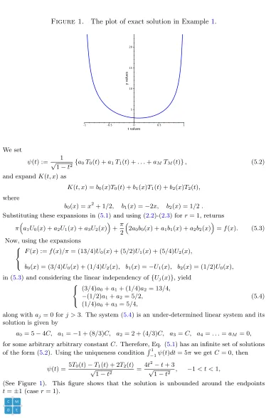
Figure 1. The plot of exact solution in Example1.

We set

ψ(t) := √ 1

1−t2 {a0T0(t) +a1T1(t) +. . .+aMTM(t)}, (5.2) and expandK(t, x) as

K(t, x) =b0(x)T0(t) +b1(x)T1(t) +b2(x)T2(t),

where

b0(x) =x2+ 1/2, b1(x) =−2x, b2(x) = 1/2. Substituting these expansions in (5.1) and using (2.2)-(2.3) forr= 1, returns

π

(

a1U0(x) +a2U1(x) +a3U2(x)

)

+π 2

(

2a0b0(x) +a1b1(x) +a2b2(x)

)

=f(x). (5.3)

Now, using the expansions

  

F(x) :=f(x)/π= (13/4)U0(x) + (5/2)U1(x) + (5/4)U2(x),

b0(x) = (3/4)U0(x) + (1/4)U2(x), b1(x) =−U1(x), b2(x) = (1/2)U0(x),

in (5.3) and considering the linear independency of{Uj(x)}, yield 

 

(3/4)a0+a1+ (1/4)a2= 13/4, −(1/2)a1+a2= 5/2,

(1/4)a0+a3= 5/4,

(5.4)

along withaj= 0 forj >3. The system (5.4) is an under-determined linear system and its

solution is given by

a0= 5−4C, a1=−1 + (8/3)C, a2 = 2 + (4/3)C, a3=C, a4=. . .=aM = 0,

for some arbitrary arbitrary constantC. Therefore, Eq. (5.1) has an inﬁnite set of solutions of the form (5.2). Using the uniqueness condition∫₋1₁ψ(t)dt= 5πwe getC= 0, then

ψ(t) = 5T0(t)−√T1(t) + 2T2(t) 1−t2 =

4t2−t+ 3 √

1−t2 , −1< t <1,

(11)

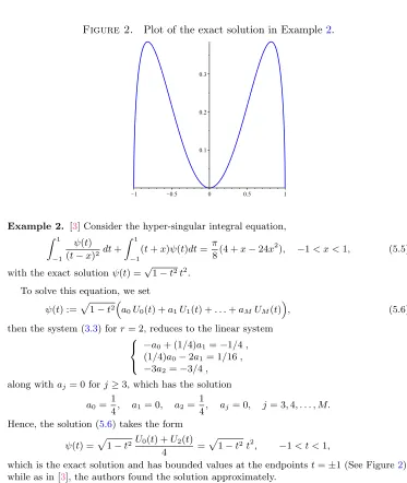
Figure 2. Plot of the exact solution in Example2.

Example 2. [3] Consider the hyper-singular integral equation,

∫ 1

−1 ψ(t) (t−x)2dt+

∫ 1

−1

(t+x)ψ(t)dt= π

8(4 +x−24x 2

), −1< x <1, (5.5)

with the exact solutionψ(t) =√1−t2_t2 .

To solve this equation, we set

ψ(t) :=√1−t2

(

a0U0(t) +a1U1(t) +. . .+aMUM(t) )

, (5.6)

then the system (3.3) forr= 2, reduces to the linear system

  

−a0+ (1/4)a1=−1/4, (1/4)a0−2a1= 1/16, −3a2=−3/4, along withaj= 0 forj≥3, which has the solution

a0=1

4, a1= 0, a2= 1

4, aj= 0, j= 3,4, . . . , M. Hence, the solution (5.6) takes the form

ψ(t) =√1−t2U0(t) +U2(t)

4 =

√

1−t2_t2_, −₁_{< t <}_1,

which is the exact solution and has bounded values at the endpointst=±1 (See Figure2), while as in [3], the authors found the solution approximately.

Example 3. The general solution of the integral equation,

∫ 1

−1 ψ(t) (t−x)2 dt+

∫1

−1 xsin(t)

t ψ(t)dt= 2πx, −1< x <1,

with one degree of freedom isψ(t) =√t3+νt

1−t2, whereν is any real number.

To solve this equation, we set

ψ(t) := √ 1 1−t2

M ∑

i=0

(12)

then solving the system (3.3) fora0, a1, . . . , aM, in the caser= 1, yield the solutions listed

in Table1, whereC1 andC2are arbitrary real constants.

Table 1. The values of multipliers of expansion (5.7).

M a0 a1 a2 a3 aj, j≥4

4 4(1−4C2) C1 0 C2 0

5 4.3636363636363636364(1−4C2) C1 0 C2 0

7 4.3488108720271800680(1−4C2) C1 0 C2 0

10 4.3491040489705664244(1−4C2) C1 0 C2 0

20 4.3491005148015315601(1−4C2) C1 0 C2 0

50 4.3491005148015315673(1−4C2) C1 0 C2 0

100 4.3491005148015315673(1−4C2) C1 0 C2 0

SettingC2=1 4, yield ψ(t) =√ 1

1−t2

(₁

4T3(t) +C1T1(t)

)

=√ 1 1−t2

(

t3+ (C1−3 4)t

)

, −1< t <1,

which is the general solution (5.7).

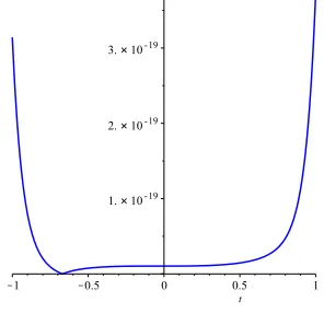
Example 4. Consider the hyper-singular integral equation

∫ 1

−1 ψ(t) (t−x)2 dt+

∫1

−1

t exψ(t)dt=−4πx+ (π/4)ex, −1< x <1,

which has the exact solutionψ(t) =ω2(t)ϕ2(t) withω2(t) =√1−t2 _and_{ϕ2(t) = 2t.} To construct an approximate solution for this equation, let

ψ(t)≃ω2(t)φ2(t), φ2(t) =

M ∑

i=0

aiUi(t).

Then solving the system (3.3) in the caser= 2, yield the functionφ2(t) for diﬀerent values ofM. ForM = 20 the error functionEM(t) =|ϕ2(t)−φ2(t)|plotted in Figure3.

Example 5. Let

∫1

−1 ψ(t) (t−x)3 dt+

∫1

−1

(2t−1)x ψ(t)dt=π, −1< x <1. (5.8)

The exact solution of this equation in the caser= 3, is given by

ψ(t) =

√

1 +t

1−t(c0V0(t) +c1V1(t) +c2V2(t) +c3V3(x)).

wherec0=c1−48c3 andc2=1 4 −c3.

To ﬁnd the approximate solution in the caser= 3, according to (1.1), we have α= 3, K(t, x) = (2t−1)x and f(x) =π.

Then we set

ψ(t) :=

√

1 +t

1−t{a0V0(t) +a1V1(t) +. . .+aMVM(t)}, and expandK(t, x) as

(13)

Figure 3. Plot of the error functionEM for Example4.

Substituting these expansions in (5.8) and using (2.2)-(2.3) forr = 3 along with (3.1) (for α= 3), returns

1 2

d2 dx2

(

a0W0(x) +a1W1(x) +. . .+aMWM(x) )

+a1b1(x) = 1.

Applying (3.2) forr= 3 and then forr= 2, and using

b1(x) = 1

2U1(x), F(x) :=f(x)/π=U0(x). yield

a0=C1−48C2, a1=C1, a2= 1

4−C2, a3=C2, a4=. . .=aM = 0

forM ≥3 and some arbitrary constantsC1 andC2. Therefore, Eq.(5.8) has an inﬁnite set of exact solutions of the form

ψ(t) =

√

1 +t 1−t

(

(C1−48C2)V0(t) +C1V1(t) + (1

4−C2)V2(t) +C2V3(x)

)

.

Example 6. Find the solution of integral equation

1 π

∫ 1

−1 ψ(t)

(t−x)3dt= 1−6x, −1< x <1, (5.9) in the caser= 4.

Letψ(t) =

√

1−t

1+tϕ(t). Then by using (3.1), Eq. (5.9) can be rewritten as

1 2π

d2 dx2

∫ 1

−1

√

1−t 1 +t

ϕ(t)

t−xdt= 1−6x, −1< x <1,

which is reduced to 1 π

∫ 1

−1

√

1−t 1 +t

ϕ(t)

t−xdt=−2x 3

+x2+c1x+c2, −1< x <1,

for some arbitrary constantsc1 andc2. Puttingc1= 1 andc2=−1

4, the right-hand side of the last equation will be 1

4W3(x), therefore, using (2.3) forr= 4, we get ϕ(t) =1

4W3(t) = 2t 3

+t2−t−1

(14)

6. Conclusions

We generalized the idea of using Chebyshev polynomials for the numerical solution of singular integral equations of the form (1.1), and solved some singular and hyper-singular integral equations to illustrate the eﬃciency of the method.

The advantages of the presented method are

• using various Chebyshev series simultaneously to solve (1.1).

• obtaining the exact solution of problem (1.1), whenever the functionsKandf are polynomials in comparison with other existing methods such as the method of [3]. • giving approximate solution with high accuracy, when the functionsK andf are

not polynomials (see the result of Example4).

Acknowledgment

The author would like to thank the respected editor and expert referees for their carefully reading and useful suggestions and comments which led to improvement of my paper. The author also would like to thank Prof. Sedaghat Shahmorad for his contribution in revising the paper and preparing the revision notes.

References

[1] S. Ahdiaghdam, S. Shahmorad and K. Ivaz,Approximate solution of dual integral equations using Chebyshev polynomials, International Journal of Computer Mathematics,94(3) (2017), 493–502.

[2] K. Atkinson and W. Han,Theoretical Numerical Analysis, Third Edition, Springer, 2009. [3] Z. Chen and Y. Zhou,A new method for solving hypersingular integral equations of the ﬁrst

kind, Applied Mathematics Letters,24(5) (2011), 636–641.

[4] S. M. Dardery and M. M. Allan,Chebyshev polynomials for solving a class of singular integral equations, Applied Mathematics,5(2014), 533–559.

[5] Z. K. Eshkuvatov and N. Long,Approximating the singular integrals of Cauchy type with weight function on the interval, Journal of Computational and Applied Mathematics,235(16) (2011), 4742–4753.

[6] M. A. Golberg,The convergence of several algorithms for solving integral equations with ﬁnite part integrals. II, Applied Mathematics and Computation,21(4) (1987), 283–293,

[7] M. A. Golberg,Numerical Solution of Integral Equations, Plenum Press, New York, 1990. [8] Y. Gong,Galerkin solution of a singular integral equation with constant coeﬃcients, Journal

of Computational and Applied Mathematics,230(2) (2009), 393–399.

[9] P. Karczmarek, D. Pylak and M. A. Sheshko, Application of Jacobi polynomials to approxi-mate solution of a singular integral equation with Cauchy kernel, Applied Mathematics and Computation,181(1) (2006), 694–707.

[10] M. Kashﬁ and S. Shahmorad,Approximate solution of a singular integral Cauchy-kernel equa-tion of the ﬁrst kind, Computational Methods in Applied Mathematics,10(4) (2010), 345–353. [11] E. G. Ladopoulos,Singular Integral Equations, Springer, Berlin, 2000.

[12] B. N. Mandal and A. Chakrabarti, Applied Singular Integral Equations, Taylor and Francis Group, CRC Press, 2011.

[13] J. C. Mason and D. C. Handscomb,Chebyshev Polynomials, Chapman and Hall, CRC Press, 2003.

[14] G. Miel, On the Galerkin and collocation methods for a Cauchy singular integral equation, SIAM Journal on Numerical Analysis,23(1) (1986), 135–143.

[15] N. I. Muskhelishvili,Singular Integral Equations, Noordhoﬀ, Groningen, 1953. [16] T. J. Rivlin,The Chebyshev Polynomials, Wiley, 1974.

(15)

[18] J. L. Tsalamengas,A direct method to quadrature rules for a certain class of singular integrals with logarithmic, Cauchy, or Hadamard-type singularities, International Journal of Numererical Modelling,25(2012), 512–524.