ABSTRACT
NORBROTHEN, EMMA MICHELE. On Classifying the Double Cosets Hk\Gk/Hk of
SL(2, k). (Under the direction of Aloysius Helminck.)
Symmetric spaces are defined as group G/H, where G is a reductive group over an algebraically closed field and H is the fixed point group of an involution θ, and are im-portant particularly in mathematics and physics. Recently the study of symmetric spaces has begun to expand to arbitrary fields and these generalizations are called symmetric k-varieties. Similarly, symmetric k-varieties are defined as the group Gk/Hk, where Gk
and Hk are thek-points of Gand H, andk is a field that is not necessarily algebraically
closed.
A problem of importance in representation theory and algebraic group theory is to describe the action of Hk on the symmetric k-variety Gk/Hk, which can be seen as
the double cosets Hk\Gk/Hk. In the Riemannian symmetric space there is the Cartan
decomposition G = HAH of the group G, where A is a maximal θ-split torus of G. Additionally, in real Riemannian symmetric spaces, allA are H-conjugate. In symmetric k-varieties, the Cartan decomposition no longer holds and not all A are necessarily Hk
-conjugate. In this thesis, we study the action of Hk on Gk/Hk for G = SL(2, k) by
studying the Hk-action on maximal θ-split tori in Gk. In particular, we study the Hk
©Copyright 2013 by Emma Michele Norbrothen
On Classifying the Double Cosets Hk\Gk/Hk of SL(2, k)
by
Emma Michele Norbrothen
A dissertation submitted to the Graduate Faculty of North Carolina State University
in partial fulfillment of the requirements for the Degree of
Doctor of Philosophy
Mathematics
Raleigh, North Carolina 2013
APPROVED BY:
Amassa Fauntleroy Thomas Lada
Ernest Stitzinger Aloysius Helminck
BIOGRAPHY
Emma Michele Norbrothen was born in Huntington, NY, to Trish Weller and Ken Nor-brothen. Shortly after the birth of her brother, Ben, the family moved to Sarasota, FL. There, Emma learned many important life lessons, like how to find sand dollars and how to tie her shoes.
As Emma and Ben began elementary school, the family moved to MA. They started in Groton, and after a year, moved to Boxborough. Emma also learned many important life lessons in these towns, like the ideas that a Halloween costume should always be winter-ready and students quiet down when fed treats.
Several years later, Emma’s parents divorced and separately moved to Acton, MA. This was a very good change for Emma, because it later meant that Matt and Karina Martel would join her family as her stepfather and sister. Moreover, Emma joined the Martel family, giving her the big-family experience she never had before and always wanted. Her dad got a cat, giving her the cat experience she never had before and always wanted.
After graduating high school, Emma migrated south to attend Gettysburg College in Gettysburg, PA. She majored in mathematics and minored in physics, and made ex-cellent friends in both departments. During all four years at Gettysburg, Emma worked in the Office of Residence Life, making several more excellent friends, and appreciat-ing another aspect of the college. Fall of her junior year, Emma studied abroad and attended Lancaster University in Lancaster, England. During her summers, Emma trav-eled to Coe College, in Cedar Rapids, IA, and Rose-Hulman Institute of Technology, in Terre-Haute, IN, to participate in Reseach Experience for Undergraduates programs. Throughout college, Emma learned many important lessons, like the value of traveling and the importance of asking questions.
special birthday lunch, Justin asked Emma for her hand in marriage.
ACKNOWLEDGEMENTS
First, I would like to thank my family. Throughout my life, they have been extremely supportive, and often believed in me more than I believed in myself. Mom, Dad, Matt, Ben, and Karina, thank you for always being there with me.
Aside from my family, I would also like to thank my best friends, in particular, Renata Sasson, Dana Ruminski, Brent Spang, and Matt Salter. Despite living on opposite sides of the country, or even the world, we have always made time for each other. Renata, Dana, Brent, Matt, thank you for your continued friendship.
I would never have gone to graduate school if it weren’t for Kathi Crow, my math ad-viser from Gettysburg. Moreover, I was motivated to become an educator/scholar/mentor by the excellent professors I had at Gettysburg and excellent teachers I had at Acton-Boxborough Regional High School. Professors like Kathi Crow, Darren Glass, and Tim Good, were my reason for choosing Gettysburg College. They embody what it means to be a teacher, a mentor, and a friend. All of my math and science teachers at Acton-Boxborough were excellent, and in particular, Peter Montalbano was the first to show me that students can learn a lot more than just math in a math classroom. Kathi, Darren, Tim, and Peter, every time I work with students, I emulate your styles.
Succeeding in my mathematics major was made easier with the help and friendship of Chloe Johnson and Lizzie Heron. The most valuable lesson I learned from them is that math is best learned when people work together, and I think about this every time I design a class. Chloe and Lizzie, thank you for the many nights of candy and chalkboards in Glatfelter 212.
Nathaniel Schwartz, Stephen Adams, Kate Brenneman, and John Hutchens, in par-ticular, helped me survive graduate school. Classes and research were much more ap-proachable with their help and friendship. Nathaniel, Stephen, Kate, and John, thank you for your friendship during what everyone said would be some of the hardest years.
Graduate school never seemed so bad when I was with Cleo or Oliver, my pet hedge-hogs. Caring for them is very humbling and rewarding. They calm me and always make me smile. Cleo and Oliver, thank you for the small joy you bring to my life every day.
This thesis would not be possible without Loek Helminck. From the moment I met him, he believed in me and all of my goals, making me even more excited about my path as a mathematician. Loek, thank you for your support, patience, passion, creativity, and friendship.
TABLE OF CONTENTS
LIST OF TABLES . . . viii
Chapter 1 Symmetric Variety Background . . . 1
1.1 A Class of Reductive Symmetric Spaces . . . 2
1.2 Our Approach to Symmetric Varieties . . . 3
1.3 Riemannian Symmetric Spaces . . . 7
1.3.1 The Subgroup Hk is Maximal Compact . . . 7
1.3.2 All Elements are Semisimple . . . 9
1.3.3 All Elements are k-split . . . 11
1.3.4 Maximal θ-split Tori are Maximal k-split . . . 12
1.3.5 All Maximal (θ, k)-split Tori are Hk-conjugate . . . 13
1.3.6 The Weyl Group has Representatives in Hk . . . 14
Chapter 2 The Hk-orbits in Qk Background . . . 18
2.1 The Hk-Action . . . 19
2.2 The Hk-orbits in Qk over Algebraically Closed Fields . . . 20
2.3 The Hk-orbits in Qk over General Fields . . . 21
2.4 The k-split Tori . . . 23
2.5 Involutions over SL(2, k) . . . 25
2.6 The (θ, k)-split Tori in SL(2, k) over General Fields . . . 29
2.7 The θ-split k-tori in SL(2, k) over General Fields . . . 31
Chapter 3 Preliminary Results about Hk-conjugation Classes in sl(2, k) 35 3.1 Characterizing Tori . . . 35
3.2 The Hk-conjugacy Classes of Type 2 Tori . . . 38
3.2.1 The Hk-conjugacy Classes of Type 2 Tori when k =R. . . 39
3.2.2 The Hk-conjugacy Classes of Type 2 Tori when k =Q . . . 39
3.2.3 The Hk-conjugacy Classes of Type 2 Tori when k =Fp . . . 40
3.2.4 The Hk-conjugacy Classes of Type 2 Tori when k =Qp,p6= 2 . . 41
Chapter 4 Characterizing Hk-conjugacy Classes of Type 3 Tori . . . 43
4.1 Characterizing Hk-conjugacy Classes of Type 3 Tori . . . 43
4.2 The Hk-conjugacy Classes of Type 3 Tori when k =Q. . . 52
Chapter 5 Type 3 Tori in sl(2, k) when k=Fp . . . 53
5.1 Examples of Type 3 Tori . . . 53
5.2 The Hk-conjugacy Classes of Type 3 Tori . . . 54
5.3 The p≡1,m≡Np Case . . . 59
5.4 The p≡3,m≡1 Case . . . 62
5.6 The p≡3,m≡Np Case . . . 67
5.7 Example Hk-conjugation Tables . . . 69
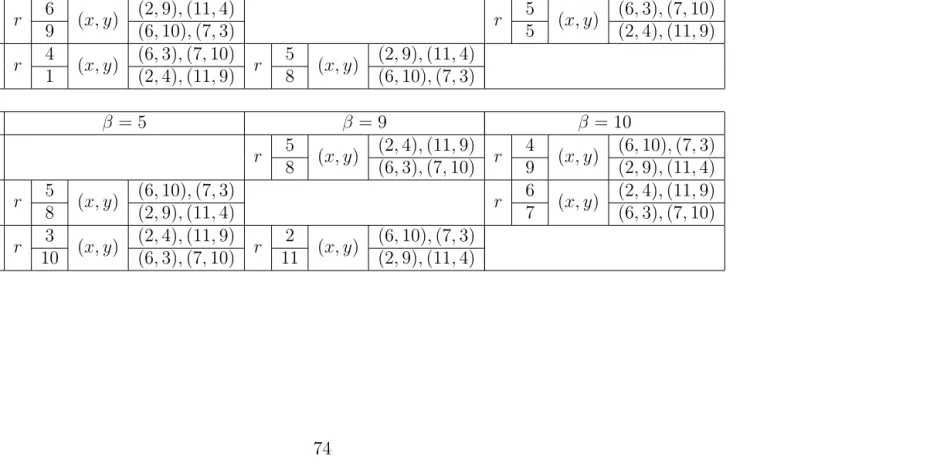
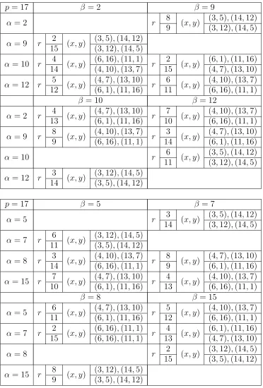
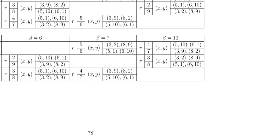
5.7.1 Example Hk-The Hk-conjugation Classes when p≡1 andm ≡Np 69 5.7.2 Example Hk-The Hk-conjugation Classes when p≡3 andm ≡1 . 72 5.7.3 Example Hk-The Hk-conjugation Classes when p≡1 andm ≡1 . 75 5.7.4 Example Hk-The Hk-conjugation Classes when p≡3 andm ≡Np 78 Chapter 6 Type 3 Tori in sl(2, k) when k=Qp, p6= 2 . . . 81
6.1 The Hk-conjugation Classes when p6= 2 . . . 81
Chapter 7 The Hk-conjugacy Classes of θ-split k-tori . . . 85
7.1 The Hk-conjugacy Classes of θ-split k-tori when k =Q . . . 85
7.2 The Hk-conjugacy Classes of θ-split k-tori when k =Fp . . . 86
7.3 The Hk-conjugacy Classes of θ-split k-tori when k =Qp, p6= 2 . . . 87
REFRENCES. . . 89
Appendix . . . 92
Appendix A Example Computations . . . 93
A.1 Computing the Hk-conjugacy Classes . . . 94
LIST OF TABLES
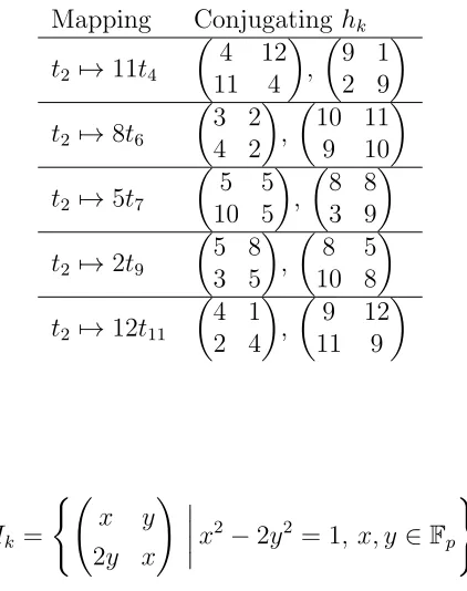
Table 5.1 The Hk-conjugation of t2 to all tori in Fp whenp= 13 and m ≡Np . 62
Table 5.2 The Hk-conjugation Classes whenp= 5 and m≡Np . . . 70
Table 5.3 The Hk-conjugation Classes whenp= 13 and m ≡Np . . . 70
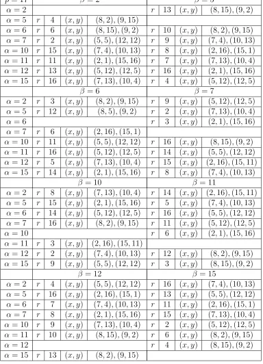
Table 5.4 The Hk-conjugation Classes whenp= 17 and m ≡Np . . . 71
Table 5.5 The Hk-conjugation Classes whenp= 7 and m≡1 . . . 73
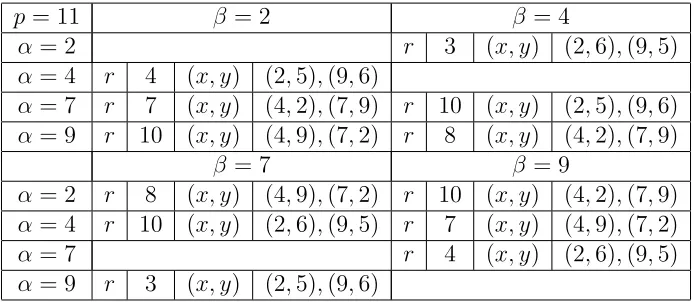
Table 5.6 The Hk-conjugation Classes whenp= 11 and m ≡1 . . . 73
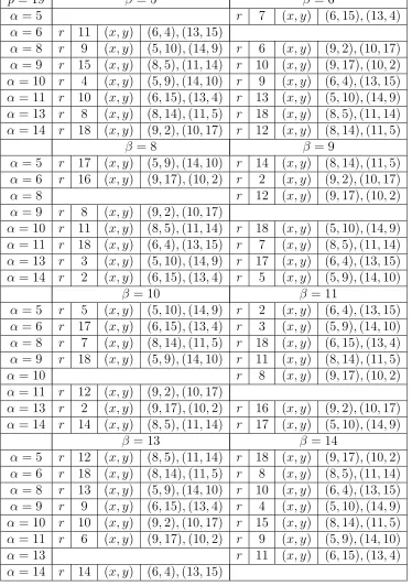
Table 5.7 The Hk-conjugation Classes whenp= 19 and m ≡1 . . . 74
Table 5.8 The Hk-conjugation Classes whenp= 5 and m≡1 . . . 75
Table 5.9 The Hk-conjugation Classes whenp= 13 and m ≡1 . . . 76
Table 5.10 The Hk-conjugation Classes whenp= 17 and m ≡1 . . . 77
Table 5.11 The Hk-conjugation Classes whenp= 3 and m≡Np . . . 79
Table 5.12 The Hk-conjugation Classes whenp= 7 and m≡Np . . . 79
Chapter 1
Symmetric Variety Background
Symmetric varieties, or the spaces of symmetries, are important in many sciences, par-ticularly in mathematics and physics. They arose around 100 years ago in physics, and were traditionally studied over the real numbers using Lie theory and analysis by Car-tan. Riemannian symmetric spaces were studied first, followed by all symmetric spaces over the reals, called affine symmetric spaces or real reductive symmetric spaces. Most of the representation theory of Riemannian symmetric spaces was developed by Harish-Chandra in [HC84]. The study of representations associated with general real reduc-tive symmetric spaces involved the work of many mathematicians, including Brylin-ski, Delorme, Flensted-Jensen, Matsuki, ¯Oshima, Sekiguchi, Schlichtkrul, and van den Ban in [vdBS97, BD92, Del98, FJ80, OS80, OM84]. Vust, Richardson, Springer, Brion, and Helminck then began researching symmetric varieties over algebraically closed fields [Vus74, Ric82, Spr98, BH00]. Symmetric k-varieties emerged in the late 1980s as a nat-ural extension, allowing symmetric spaces and their representations to be studied over fields other than the reals and complexes, like the finite and p-adic fields, see [HW93]. For results of symmetric k-varieties over the finite fields, see [Gro92] and [Lus90]. For results of symmetric k-varieties over p-adic fields, see [HHa, JLR93, RR96].
see [HHb].
Let G be a reductive algebraic group defined over a field k, and take θ ∈ Aut(G) to be an involution on G. The space Q={xθ(x)−1|x∈G} is a subvariety of G, called the
symmetric variety. LetH=Gθ be the fixed point group ofθinG. Then the homogeneous
spaceG/H is isomorphic to the symmetric varietyQ. The symmetrick-variety is the space Qk ={xθ(x)−1| ∈Gk}, whereGkis thek-rational points ofG. Similarly, takingHkto be
the k-rational points ofH, we get thatQk 'Gk/Hk. The definition of symmetric variety
can be extended even further to general groups G, in which case, the spaces Q 'G/H are called the generalized symmetric space. The double cosets Hk\Gk/Hk can be seen
as Hk acting on the coset space Gk/Hk, or Hk acting on the symmetric variety Qk. To
study symmetric k-varieties, and then the Hk-action on symmetrick-varieties, we begin
by reviewing symmetric varieties.
In this thesis, we study the double cosets Hk\Gk/Hk over the rational, finite, and
p-adic fields. To study these, we first review symmetric varieties. We begin by reviewing a classical approach to symmetric spaces and then a broader approach to symmetric varieties. To conclude our review of symmetric varieties, we discuss a prominent type of symmetric varieties, called the Riemannian symmetric space. Riemannian symmetric spaces are of particular importance due to their formulation and resulting characteristics.
1.1
A Class of Reductive Symmetric Spaces
Let k = R and let V = kn be an n-dimensional vector space over k. Let M
n(k) be the
set ofn×n matrices with entries in k. Then
GL(n, k) = {A∈Mn(k)| det(A)6= 0}
is the set of invertible matrices in Mn(k). Let id∈GL(n, k) be the identity matrix.
Let B be a nondegenerate bilinear form on V. Thus, for x, y ∈ V, B(x, y) = xTM y for some M ∈ GL(n, k). Moreover, take B to be symmetric, thus M = MT. Take some A ∈ Mn. Then B(Ax, y) = B(x, A0y) for some A0, and call A0 the adjoint of A. We get
that A0 = M−1ATM, and note that when M = id, we get A0 = AT. The matrix A is
O(V, B) = {A∈GL(n, k)|A0A = id}.
Define a map τ : GL(n, k) → GL(n, k) by τ(A) := AA0. Then the kernel of τ is ker(τ) =τ−1(id) = O(V, B). The image of τ is Im(τ) ={AA0|A ∈GL(n, k)}, which we
call Q(V, B) = Im(τ). We get
GL(n, k)/O(V, B)'Q(V, B), and we call Q(V, B) a reductive symmetric space.
This approach to symmetric spaces was first constructed over the reals. These results can generalize to any field k.
1.2
Our Approach to Symmetric Varieties
The bilinear form construction to symmetric varieties is limited because it leads only to outer automorphisms in Aut(G). There are more ways to construct symmetric varieties. We choose to define symmetric varieties based on involutions over algebraic groups. Notation. Letk be a field of characteristics not equal to 2, let Gbe a reductive algebraic group defined overk, and let Gk be the k-rational points ofG. Let Aut(G) be the set of
all automorphisms ofG.
Definition 1.2.1. An involutionof G is an automorphism θ∈Aut(G) ofG such that θ2 = id yetθ 6= id. A k-involutionof G is an involution ofG that sends Gk to Gk.
Let θ ∈Aut(G) be an involution of G, or a k-involution when k is not algebraically closed. Let H =Gθ ={g ∈ G|θ(g) =g} be the fixed point group of θ in G, and let H
k
be the k-rational points of H. By a result of Steinberg in [Ste68], H0 is reductive, which
then implies that H itself is reductive.
Definition 1.2.2. For an involution θ, the symmetric variety is defined to be the subvariety Q = {xθ(x)−1|x ∈ G}. This space is isomorphic to G/H, thus Q ' G/H,
and both are referred to as the symmetric variety.
Proposition 1.2.1. There is an isomorphism between the generalized symmetric space G/H and Q.
Proof. Letτ :G→G be defined by
τ(g) :=g∗e=gθ(g)−1, (1.1)
where g ∈G. For x, y ∈G,
τ(x) = τ(y) ⇐⇒ xy−1 =θ(x)θ(y)−1 ⇐⇒ xy−1 ∈H Thus,τ−1(τ(x)) = xH for any x∈G. Therefore, Q'G/H.
Richardson showed this is an isomorphism of varieties as well.
Assumed in the definition of symmetric variety is the idea that G, H, and Q are taken over the algebraic closure of the base fieldk. Restricting these spaces to just their k-points changes the nature of these spaces considerably, warranting the definition below.
Definition 1.2.3. LetGk andHk be thek-rational points ofGandH, respectively, and
θ ∈Aut(Gk). Let Qk={xθ(x)−1|x∈Gk}. ThenQk 'Gk/Hk is called the symmetric
k-variety, and is a generalization of symmetric spaces to general fieldsk.
When we take Qk ' Gk/Hk to be the symmetric k-variety, this is an isomophism
of reductive varieties, making the proof of Proposition 1.2.1 more complicated. For the proof, see [Ric82].
Definition 1.2.4. LetG be a real reductive group. For an involutionθ, thesymmetric space is defined to be subspace Q = {xθ(x)−1|x ∈ G}. This space is isomorphic to
G/H, thusQ'G/H, and both are referred to as the symmetric space.
There are many examples of symmetric spaces, symmetric varieties, and symmetric k-varieties. We first consider a well-known decomposition of GL(n, k).
Example 1.2.1. Letk =Rand take Gk = GL(n,R). Consider the involution
θ(x) = (xT)−1
for all x ∈ Gk. Then Hk = {x ∈ Gk|xxT = id} = O(n,R). The symmetric k-variety is
which is the decomposition of real invertible matrices into the product of orthogonal matrices and symmetric positive-definite matrices.
Throughout this thesis, G is assumed to be a reductive algebraic group, including in the given definitions of symmetric variety, symmetric k-variety, and symmetric space. The notion of symmetric spaces can, in fact, extend to any group. For the following definition, temporarily drop the assumption that Gis a reductive algebraic group. Definition 1.2.5. Let G be a group. Let θ ∈ Aut(G) an involution of G, H = Gθ the fixed point group of θ inG, and Q={xθ(x)−1|x∈G}, as before. ThenQ'G/H, and both are referred to as the generalized symmetric space.
We can define a generalized symmetric space for any group. In fact, any group can itself be seen as a generalized symmetric space.
Example 1.2.2. Let G be a group and consider the group G×G. Take the involution θ(x, y) = (y, x) for all (x, y) ∈G×G. Define an automorphism τ : G×G→ G×G by τ := (x, y)·θ(x, y)−1. Then H = ker(τ) = {(x, x)|x∈G} 'Gand
Q= Im(τ) = {(x, y)·θ(x, y)−1|(x, y)∈G×G} ' {(x, x−1)|x∈G}. Notice that Q'G, thusG itself can be viewed as a generalized symmetric space.
We construct Q by acting θ on G. The space defined below helps us classify how θ acts on G.
Definition 1.2.6. LetG be a group andθ∈Aut(G) an involution ofG. Theextended symmetric space of G is the spaceR ={g ∈G|θ(g) =g−1}.
The action of θ on an element xθ(x)−1 ∈ Q is θ(xθ(x)−1) = θ(x)x−1 = [xθ(x)−1]−1. Thus, the symmetric space Q is contained within R, hence the name. While we conven-tionally differentiate between symmetric spaces, symmetric k-varieties, and generalized symmetric spaces, we refer to the setRas the extended symmetric space in all situations. Also, if the groupGis has a topology and is connected, thenQis also connected because it is the image ofτ acting on G. Contained in Qis the identity, making Qthe connected identity component of R, that is, Q = R0. Thus, Q = R0 when k = ¯k is algebraically
Throughout this thesis, we will study k-tori inside symmetric k-varieties, for they provide valuable information about the structure and behavior the symmetrick-varieties. As we will see throughout this chapter, there are many results about tori inside symmetric varieties, Riemannian symmetric spaces in particular, and many of these results do not translate to k-tori in symmetric k-varieties. Thus, we now focus on tori. For an arbitrary fieldk, we will refer to tori ask-tori to emphasize the field over which the tori are defined. In a construction of Q, we act θ on G. Thus, we are very interested in the action of θ on tori in G, and this leads us to the following definitions.
Definition 1.2.7. Given an involution θ ∈ Aut(G) where G is a group, a torus T is θ-stable if θ(T) = T.
An element inside the symmetric spaceQ⊆R has the property that θ sends it to its inverse. Thus, we define the following property for tori.
Definition 1.2.8. Let T ⊂G be a torus and θ ∈ Aut(G) an involution. We say that T is θ-split if θ(t) = t−1 for every t∈T.
Note that θ-split tori are θ-stable by definition. LetT be a torus and let
T+ ={t ∈T |θ(t) =t}0; (1.2)
T− ={t ∈T |θ(t) =t−1}0. (1.3)
ThenT =T+T−, andT+∩T− is finite. Note that this is a group-theoretic version of an
eigenspace decomposition.
A k-torus T can also be decomposed as T =TaTd, where Ta is k-anisotropic and Td
is k-split [Bor91].
Definition 1.2.9. LetG be a group defined over k, T ⊂G a torus, and θ∈Aut(G) an involution. The torusT is (θ, k)-splitif it is both θ-split and k-split.
1.3
Riemannian Symmetric Spaces
Symmetric varieties first arose over the real numbers. Specifically, the first symmetric variety that mathematicians researched was the Riemannian symmetric space because it arises naturally from differential geometry. The Riemannian symmetric space has many nice properties, and often when studying symmetrick-varieties, we are in search of prop-erties analogous to those in the Riemannian symmetric space, should such propprop-erties exist. Thus, we review Riemannian symmetric spaces, and most of these results can be found in [Hel01] and [HW93].
Throughout this section, assume k =R. Letg =L(G), h =L(H), and q=L(Q) be the Lie algebras of G, H, and Q, respectively. Let Gk be a real Lie group.
Definition 1.3.1. Let θ ∈ Aut(G) be an involution, Hk = Gθk the fixed point group of
θ inGk, andAk aθ-stable maximal k-split torus. Then θ is aCartan involution if the
following three properties hold.
1. The subgroup Hk is maximal compact.
2. We have (k∗)2 = (k∗)4.
3. There exists a Cartan decomposition Gk=HkAkHk.
Definition 1.3.2. LetGk be a real Lie group. Take θ∈Aut(Gk) to be a Cartan
involu-tion. LetHk =Gθk be the fixed point group ofθinGk, and takeQk ={xθ(x)−1|x∈Gk}.
Then Qk'Gk/Hk is the Riemannian symmetric space.
1.3.1
The Subgroup
H
kis Maximal Compact
We will review several important properties of Riemannian symmetric spaces, many of which stem from the property below.
Property 1. In a Riemannian symmetric space Qk, the fixed point group Hk is maximal
compact.
Example 1.3.1. Let Gk = SL(2,R) and take the involution θ(x) = (xT)−1. Then the
fixed point group is Hk = (
a b
−b a
!
a2+b2 = 1, a, b ∈R )
We can conclude Property 1 from the following results in [Hel01].
Proposition 1.3.1. Every semisimple Lie algebra g over C has a real form which is compact.
A real Lie algebra g is semisimple if and only if its killing form κ is nondegenerate. Takek⊂g to be a maximal compact subalgebra. Let p=k⊥, and note that κ restricted top is positive definite. Then g=k⊕p is the ±1 eigenspace decomposition. Let gC⊃g be the complexification ofg and σ the conjugation of gC that leaves g invariant.
Lemma 1.3.1. Let g = k⊕p be a real Lie algebra, gC its complexification, and σ the conjugation of gC that leaves g invariant. Then there exists a compact real form of gC
that is σ-stable.
To prove Lemma 1.3.1, defineu=k⊕ip, and note thatipis now negative definite. Let τ denote the conjugation of gC with respect tou. Then σ(u) =u if and only if στ =τ σ. Thus,στ is of order 2, and moreover, it is a Cartan involution, leaving gστ =k.
Lemma 1.3.1 shows how to construct a Cartan involution. Combining Proposition 1.3.1 and Lemma 1.3.1 shows that each semisimple real Lie algebra has a Cartan decom-position. Moreover, one always has a maximal compact subalgebra, as shown below in Theorem 1.3.1, which proves Property 1 above.
Theorem 1.3.1. Let g0 be a semisimple Lie algebra over R which is the direct sum
g0 =k0 +p0, where k0 is a subalgebra and p0 is a vector space. The following conditions
are equivalent.
1. The decomposition g0 =k0+p0 is a Cartan decomposition.
2. The mapping s0 :T +X →T −X, where T ∈k0 and X ∈p0, is an automorphism
of g0 and the symmetric bilinear form
Bs0(X, Y) = −B(X, s0Y)
is strictly positive definite, that is, B <0 on k0 and B >0 on p0.
Many of the other important properties of the Riemannian symmetric space follow from the result thatHk is maximal compact. As we will see in this section and throughout
this thesis, not all of these properties generalize to symmetric k-varieties. In fact, the property the Hk is maximal compact does not necessarily generalize to symmetric
k-varieties, as Examples 1.3.2 and 1.3.3 below demonstrate.
Example 1.3.2. Let Gk = SL(2,C) and take the involution θ(x) = (xT)−1. Then the
fixed point group is Hk = (
a b
−b a
!
a2+b2 = 1, a, b∈
C
)
, which is noncompact.
Examples 1.3.1 and 1.3.2 differ only by the choice of the base field. In Example 1.3.1, we assumedk =R, which is the base field in a Riemannian symmetric space. In Example 1.3.2, we went up to k = ¯R, and this was enough to break the compactness quality of Hk.
Notation. We will use the notation Int(A) to mean conjugation by A∈GL(n, k). Note that θ(g) = (gT)−1 for all g ∈ G
k, the involution used to define a Riemannian
symmetric space, is equivalent to θ(g) = Int(A)(g) with A = 0 1
−1 0
!
for all g ∈ Gk.
Now we consider a Lie group with a different involution.
Example 1.3.3. LetG= SL(2,R) and take the involutionθ = Int(A) withA = 0 1 1 0
!
. Then the fixed point group is
Hk = ( x y y x !
x2−y2 = 1
)
=
(
coshφ sinhφ sinhφ coshφ
!
φ∈R )
,
which is noncompact. Thus, we can see that by simply switching to another involution, and thereby switching to a symmetrick-variety, we lose the property thatHk is maximal
compact.
1.3.2
All Elements are Semisimple
Below is a fundamental result of the compactness of the fixed point group Hk.
Example 1.3.4. Let Gk = SL(2,R) and take θ(g) = (gT)−1 for all g ∈ Gk. Then the
Riemannian symmetric space Qk ={xxT |x∈G} is the set of symmetric matrices with
positive real eigenvalues, and thus consists of semisimple elements.
Property 2 is a result of the following theorem, which was proven by Cartan. In [Hel01] and [HW93] it has been generalized to symmetric k-varieties such that the characteristic of k is not 0. Note that Property 1 satisfies the condition thatH is anisotropic over R. Theorem 1.3.2. LetGbe a connected reductive algebraic group overksuch that ch(k) = 0, Q={xθ(x)−1|x∈G}, and g=h+q the decomposition of g=L(G) into eigenspaces of θ. Suppose that H is anisotropic over k. Then the following conditions are true.
1. The symmetric k-variety Qk consists of semisimple elements.
2. The symmetric k-variety qk consists of semisimple elements.
In fact, for a maximal compact subgroup Hk ⊂ Gk, the space Gk/Hk is going to
consist of semisimple elements. This does not generalize to symmetrick-varieties over an arbitrary field k.
Example 1.3.5. As in Example 1.3.3, let k = R, G = SL(2,R), and θ = Int(A) with A= 0 1
1 0
!
. In this case, the symmetrick-variety is
Qk= (
a2−b2 bd−ca
ca−bd d2−c2
!
a, b, c, d∈R, ad−bc= 1
)
,
which contains non-symmetric matrices and non-semisimple elements. For instance, the values a = 1, b = 2, c = 0, and d = 1 create the matrix −3 2
−2 1
!
with Jordan normal
form −1 1 0 −1
!
, which is not semisimple.
The elements in the Riemannian symmetric space Qk are semisimple, and thus
con-tained in a torus ofG. Therefore, to study elements inQk ⊂R, we can studyθ-splitk-tori
1.3.3
All Elements are
k
-split
In a Riemannian symmetric space, semisimplicity implies the following condition. Property 3. All elements in a Riemannian symmetric space Qk are k-split.
By Property 2, all elements in the Riemannian symmetric space are semisimple, and now we see that they are also k-split.
Example 1.3.6. As in Example 1.3.4, let Gk = SL(2,R) and take θ(g) = (gT)−1 for all
g ∈Gk, creating the Riemannian symmetric space Qk ={xxT |x∈ G}. These elements
are symmetric matrices with positive real eigenvalues and can be diagonalized over the base field. Hence they are k-split.
By Property 1.3.1, the real Lie group Gk has an associated Cartan decomposition,
allowing us to apply the following theorem.
Theorem 1.3.3. Let H be compact, let A be a θ-stable maximal k-split torus of G, and let Gk = HkAkHk. Then the Riemannian symmetric space Qk = {xθ(x)−1|x ∈ Gk}
consists of k-split semisimple elements.
This result is fundamental to this thesis, because in Riemannian symmetric spaces, semisimplicty implies that elements will split overR. As we saw in Example 1.3.5, not all elements in symmetrick-varieties are semisimple. Further, in a symmetrick-variety, even those that are semisimple might not bek-split. For an example, we turn to Lie algebras. Example 1.3.7. Let gk = sl(2,R) and take θ = Int(A) with A =
0 1 1 0
!
. Then the symmetrick-variety is
qk = (
a b
−b −a
!
a, b∈k
)
.
The element 0 1
−1 0
!
has minimum polynomialx2+ 1 and is hence semisimple, yet has eigenvalues ±i, and thus is not split over R.
1.3.4
Maximal
θ
-split Tori are Maximal
k
-split
We know that elements in Qk are semisimple, k-split, and θ-split in a Riemannian
sym-metric space. This leads us to the following property.
Property 4. In a Riemannian symmetric space Qk, all maximal θ-split tori are maximal
k-split.
Example 1.3.8. As in Example 1.3.1, letGk = SL(2,R) andθ(g) = (gT)−1for allg ∈Gk
to create the Riemannian symmetric space Qk ={xxT |x∈G}. The torus
T =
(
x 0 0 x−1
!
x∈R∗
) ⊂Qk
is contained in Qkand is θ-split. Also notice thatT is maximal inGk. In this form of the
torus, we can see that all elements split over R, too.
Theorems 1.3.3 allows us to apply the following theorem, which results in Property 4 above.
Theorem 1.3.4. Assume Qk consists ofk-split semisimple elements. Then the following
are true.
1. All θ-split tori of G are k-split.
2. All maximal θ-split tori of G are maximal (θ, k)-split.
3. Given any x∈Qk, there is a maximal (θ, k)-split torus of G containing x.
All elements in the Riemanninan symmetric space Qk are semisimple and k-split,
hence they are contained in k-split tori. We know that Qk is θ-split because Qk ⊂ R,
thus elements in Qk are contained in (θ, k)-split tori of Gk.
Once again, these properties do not hold in symmetric k-varieties. For an example, we turn to Lie algebra.
Example 1.3.9. As in Example 1.3.7, let gk = sl(2,R) and take θ = Int(A) with
A= 0 1 1 0
!
. Then the symmetric k-variety is
qk = (
a b
−b −a
!
a, b∈k
)
One of the toral subalgebras inside qk is
t=
(
0 x
−x 0
!
x∈k
)
.
The Lie algebra equivalent of aθ-split torus is a toral subalgebra such thatθ(t) =−t for all t ∈ t, and note that the toral subalgebra above is indeed θ-split. The eigenvalues of the matrices inside t are ±ix, hence the elements are semisimple and yet this maximal toral subalgebra does not split over R.
Theorem 1.3.4 shows us that because elements in Qk are semisimple and k-split,
θ-split tori are k-split. Proposition 1.3.2 below shows reverses this, showing that k-split tori must be θ-split as well.
Proposition 1.3.2. LetHbe compact and Gk=HkAkHk, whereAis aθ-stable maximal
k-split torus of G, as in the Riemannian symmetric space. Then A is maximal θ-split.
1.3.5
All Maximal
(
θ, k
)-split Tori are
H
k-conjugate
In this thesis, we study maximal θ-split k-tori. We review what is known about (θ, k)-split tori, and then focus on θ-split k-anisotropic tori. In particular, we analyze the Hk
-conjugation ofk-tori. The following result aboutHk acting onθ-split tori in Riemannian
symmetric spaces is of fundamental importance to this thesis, because, once again, it does not hold over symmetric k-varieties.
Property 5. In a Riemannian symmetric space Qk, all maximal (θ, k)-split tori are
Hk-conjugate.
Example 1.3.10. Let Gk = SL(2,R) and θ(g) = (gT)−1 for all g ∈ Gk. In Example
1.3.3, we considered the torus
T =
(
x 0 0 x−1
!
x∈R∗ )
.
That is because all maximal (θ, k)-split tori in inGk are conjugate to this form, allowing
us to only consider the torus T.
Proposition 1.3.3. Let Hk be k-anisotropic andGk =HkAkHk. Then any two maximal
(θ, k)-split tori are conjugate by an element of H0 k.
In symmetric k-varieties, maximal k-tori are not alwaysHk-conjugate.
Example 1.3.11. In [BH09], Beun and Helminck showed that there is an infinite number of Hk-conjugacy classes of (θ, k)-split tori in SL(2,Q).
We can extend Proposition 1.3.3 to create the theorem below. Let θ ∈Aut(G) be an involution ofG, though not necessarily a Cartan involution.
Theorem 1.3.5. Let θ be an involution of G defined over k andH0 the identity
compo-nent of theθ fixed point group,Gθ. IfG has a Cartan involution overk, then all maximal
(θ, k)-split tori are Hk-conjugate.
Theorem 1.3.5 shows us that as long as the group G has a Cartan involution, all of its tori are conjugate by the fixed point group, even if the tori and the fixed point group are created using a non-Cartan involution. In symmetrick-varieties, this is far from true.
1.3.6
The Weyl Group has Representatives in
Hk
Property 6. Let Qk be a Riemannian symmetric space and T a maximal θ-split torus.
The Weyl group W(T) has representatives in WHk(T).
Example 1.3.12. LetGk = SL(2,R) and take torus T = (
x 0 0 x−1
!
x∈R∗
)
. Then the Weyl group ofT is
W(T) =N(T)/T =
(
id, 0 1
−1 0
!)
.
The fixed point group is Hk = (
a b
−b a
!
a2+b2 = 1 )
. Notice that the conditions a = 0 or b = 0 give us the following matrices when combined with the requirement a2+b2 = 1.
a= 0 ⇒ ha =
0 1
−1 0
!
b = 0 ⇒ hb =
1 0 0 1
!
Notice thatha, hb ∈W(T) and ha, hb ∈NH(T), showing that both elements ofW(T) are
represented in WHk(T).
Borel and Tits give us the following theorems.
Theorem 1.3.6. Let A be a maximal k-split torus. Then W(A) has representatives in WGk(A).
Theorem 1.3.7. For an involutionθ, let A be a maximal θ-split torus and H be its fixed point group in G. Then W(A) has representatives in WH(A).
Property 6 is a result of the following theorem in [HW93], which is an extension of Theorems 1.3.6 and 1.3.7.
Theorem 1.3.8. For a Cartan involution θ, let A be a maximal (θ, k)-split torus and H be its fixed point group in G. Then W(A) has representatives in WHk(A).
When working over a general field k and with a general involution θ, elements in the Weyl group are not necessarily in the fixed point group. Below is an example of when it does not hold.
Example 1.3.13. Let Gk = SL(2,Fp) with p = 5 and θ = Int(A) with A =
0 1 2 0
!
. The fixed point group of θ inGk is
Hk = (
x y 2y x
!
x2−2y2 = 1, x, y ∈Fp )
.
Take the torus T =
(
x 0 0 x−1
!
x∈F∗
p )
, and the Weyl group of T
WGk(T) =NGk(T)/T =
(
id, 0 1
−1 0
!)
.
Notice that the second Weyl group element has form 0 1 4 0
!
, which does not fit the form ofHk. Thus, not all elements in WGk(T) are contained in Hk.
Note that in Riemannian symmetric spaces and symmetrick-varieties whenk is alge-braically closed,WG(T) = WH(T), forT a maximal torus. The Weyl group in H counts
Proposition 1.3.4. Let Hk be maximal compact, T a maximalθ-split torus, and t∈T.
Then Hk·t∩T =WHk(T)·t.
Proof. Consider h1·t = h1th−11 ∈ Hk·t∩T, where h1 ∈Hk. All tori are Hk-conjugate,
thush1T h−11 =T1, whereT1 is another maximal torus inGk. By construction,h1T h−11 ⊂
ZGk(h1th
−1
1 ) andT ⊂ZGk(h1th
−1
1 ). Thus, the toriT andT1areHk-conjugate inZGk(h1th
−1 1 )
as well. Therefore, there exists anh2 ∈Hk∩ZGk(h1th
−1
1 ) such thath2T1h−21 =T1. Putting
these together, we see that there exists an h ∈ NHk(T) such that h1 ·t = h·t, namely
h = h2h1. Thus, Hk ·t∩T ⊂ WHk(T)·t. The agrument reverses, hence Hk·t∩T =
WHk(T)·t.
Example 1.3.14. Let Gk = SL(2,R) and take torus T = (
x 0 0 x−1
!
x∈R∗
)
. Con-sider the fixed point group Hk and Weyl group WGk(T) from Example 1.3.12. We know
that fort∈T,Hk·t∩T =WHk(T)·t. When we considerHk·t∩T, we get the following
relations:
abx=abx−1
(a2x+b2x−1)(a2x−1+b2x) = 1.
The implication of these relations is that a = 0, or b = 0, or x = ±1. Combining these relations with the requirement that a2+b2 = 1, we create h
a, hb ∈ Hk as in Example
1.3.12, showing the Hk-orbits intersect the torus T twice.
The proof of Proposition 1.3.4 uses the fact that in a Riemannian symmetric space, all tori are Hk-conjugate. Thus, this relation does not necessarily hold in a symmetric
Chapter 2
The
H
k
-orbits in
Q
k
Background
The generalizations of symmetric spaces to an arbitrary field k are called symmetric k-varieties, which arise in many areas of mathematics and physics, and play a particularly important role in representation theory and number theory. In the past thirty years, the study of symmetrick-varieties has begun to expand, unveiling many open questions. Many of these open questions are about how the structure of symmetric spaces can be generalized to symmetric k-varieties, if at all. Some of the structure of symmetric k-varieties that is important to representation theory and number theory is how Gk and
Hkact onQk 'Gk/Hk. In this thesis, we analyze howHkacts on the symmetrick-variety
Gk/Hk.
In [Ric82], Richardson analyzes the action ofH on the symmetric spaceG/H whenG is a group defined over an algebraically closed field. Helminck and Wang the transition to symmetric k-varieties by analyzing Gk/Hk over fields of characteristic p. Helminck and
Schwarz study orbits of symmetric groups in symmetric k-varieties over algebraically closed fields and the real numbers [HS09, HS02, HS04, HS11]. The results of [Ric82] and [HS11] show that we can begin to study the movements of elements in Gk/Hk by
analyzingθ-split k-tori inGk/Hk, whereθ is a k-involution on Gk. In [BH09], Beun and
Notation. Let G be a reductive algebraic group over an algebraically closed field. Let θ ∈ Aut(G) be an involution on G, thus θ2 = id, and let H = Gθ be the fixed point
group of θ in G. The subvariety Q={xθ(x)−1 | x∈G} can be identified with the coset
space G/H, and both are called the symmetric variety. Let g = L(G), h = L(H), and q = L(Q) be the Lie algebras of G, H, and Q, respectively. When working over a field that is not algebraically closed, Gk,Hk,gk, andhk denote thek-rational points of G,H,
g, and h, respectively. Then Qk ={xθ(x)−1|x∈Gk} and qk ={x−θ(x)|x∈gk}.
2.1
The
H
k-Action
In this thesis, we examine Hk acting on the symmetric k-variety Qk'Gk/Hk. Note that
G and H act on the symmetric variety G/H by left multiplication. There are two other actions byGandH onG/H 'Qthat are important when working in symmetric spaces: conjugation and twisted conjugation.
Notation. Takeg, x∈G. The action of conjugation of xbyg is denoted by g·x=gxg−1.
Definition 2.1.1. Take g, x ∈ G and let θ ∈ Aut(G) be an involution. The action of θ-twisted conjugation of x byg is g∗x=gxθ(g)−1.
Recall that Q={xθ(x)−1|x ∈G}, thus, we can view Q as G∗e, the G-orbit of the
identity. In particular, the θ-twisted conjugation is an important mapping from Q toQ, because for g ∈ G and x ∈ Q, we find that g∗x ∈ Q and g ·x 6∈ Q. Thus, θ-twisted conjugation is a conjugation mapping that allows Q to go to Q. When conjugating by the fixed point group H, conjugation and θ-twisted conjugation are the same action.
In general, for x ∈ G, we have the Jordan decomposition x = xxxu, where xs is
semisimple, xu is unipotent, and xs, xu ∈ G. In [Ric82], Richardson shows that this
decomposition holds even when restricted to the symmetric space.
Theorem 2.1.1. Consider x = xsxu. Then x ∈ Q = {xθ(x)−1|x ∈ G} if and only if
xs, xu ∈Q.
The proof of this theorem relies on the uniqueness of the Jordan decomposition. Richardson uses the map τ :G→G, defined by
as in 1.1, to show thatx, xs, andxu are inQ. This theorem is significant because it shows
that we can analyze elements in the symmetric space by first analyzing the semisimple elements and the unipotent elements. In [Ric82], Richardson gives some structure to these semisimple elements by linking them to θ-split tori.
2.2
The
H
k-orbits in
Q
kover Algebraically Closed
Fields
Recall that a θ-split torus T is a torus such that θ(t) = t−1 for all t ∈ T. In older
literature, the concept that we define as a θ-split torus is referred to as a θ-anisotropic torus. Anisotropic is the algebra equivalent of compact. Thus, a torus that is θ-split can also be compact, and a θ-split toral subalgebra can also be anisotropic. For this reason, the terminology has shifted fromθ-anisotropic toθ-split, and this shift begins in Springer and Helminck literature. In [Vus74], Vust shows that such tori exist.
Lemma 2.2.1. In a nontrivial group G, there exists a nontrivial θ-split torus.
LetT be aθ-split torus. Thenτ(T)⊆T because θ(τ(t)) =t−2 =θ(t)t−1 =τ(t)−1 for any t ∈T. When G is over k an algebraically closed field, or k such that (k∗)2 = (k∗)4,
these sets are equal. Note that τ(T) ⊂ Q by definition, and when working over an algebraically closed field, this implies that τ(T) =T ⊆Q.
Example 2.2.1. Letk =Fp for some prime p and letG= GL(2, k). Consider the torus
T =
(
x 0 0 y
!
x+y 6= 0, x, y ∈Fp )
Then τ(T) =
(
x2 0 0 y2
!
x, y ∈Fp )
. Thus, τ(T)(T.
In [Ric82], Richardson presents the theorem below. It provides important structure for studying semisimple elements inside of the symmetric spaceQ by linking semisimple elements to tori.
Theorem 2.2.1 is fundamental to this thesis. Every semisimple element in Q is con-tained in a θ-split torus, thus we can study semisimple elements by studying θ-split tori, which will ultimately help us study general elements in Q.
When we study H acting on Q ' G/H, because of Theorem 2.1.1, we can study H acting on semisimple elements in Q. In order to study this action on semisimple elements, we can study the H action on θ-split tori of G contained in Q by Theorem 2.2.1. In particular, a maximal θ-split torus is a torus that is maximal when compared with other θ-split tori. Throughout this thesis, let Aθ denote the set of maximal θ-split
tori in G, and let A∈ Aθ be a maximal θ-split torus. In the theorem below, Vust shows us how H acts on these maximal θ-split tori.
Theorem 2.2.2. Let A1, A2 ∈ Aθ be maximal θ-split tori in G. Then there exists an
h∈H0 such that h·A
1 =A2.
This result is of fundamental importance in this thesis. Vust shows that all maximal θ-split tori are H-conjugate when the field is algebraically closed. Over general fields, this result does not hold, that is, there is sometimes more than oneHk-conjugacy class of
maximalθ-split k-tori. In this thesis, we begin to determine when maximal θ-split k-tori are Hk-conjugate, that is, how H-conjugacy classes break up into Hk-conjugacy classes.
2.3
The
H
k-orbits in
Q
kover General Fields
In the field of symmetric spaces, Riemannian symmetric spaces were first studied be-cause they arise naturally over the reals. While Riemannian symmetric spaces are not technically defined over an algebraically closed field, many of their properties also hold in symmetric spaces when k is algebraically closed. Many of these properties do not necessarily hold in symmetrick-varieties over general fields.
One such property in the Riemannian symmetric space is that the fixed point group Hk is compact. In general fields k, the equivalent property is that Hk is k-anisotropic.
When Hk is k-anisotropic, many of the additional properties of Riemannian symmetric
spaces still hold.
Over general fields, including the reals, Hk is not always compact or k-anisotropic.
compact, whereas in Example 1.3.3 we used a non-Cartan involution, and the resulting fixed point group was noncompact. Therefore, throughout this thesis, assume Hk is not
k-anisotropic, unless we explicitly state otherwise.
As we saw in Property 2, in a Riemannian symmetric space, Qk consists only of
semisimple elements. In [Hel10], Helminck shows that this property translates to sym-metric k-varieties when Hk is k-anisotropic and the characteristic of the field k is zero.
Theorem 2.3.1. Let k be a field such that ch(k) = 0. Let G be a connected reductive algebraic group over k. For an involution θ ∈ Aut(G), let Q= {xθ(x)−1|x∈ G} be the
symmetric space. For g =L(G), we have the eigenspace decomposition g=h+q, where h=L(H). Assume H is k-anisotropic. Then the following conditions are true.
1. The symmetric k-variety Qk consists of semisimple elements.
2. The symmetric k-variety qk consists of semisimple elements.
Below are some examples demonstrating that the condition that Hk isk-anisotropic
is necessary. Recall that for g ∈ G and A ∈ GL(n, k), the notation Int(A)(g) denotes A·g.
Example 2.3.1. Let k = R and G = SL(2,R). Take the involution θ(g) = (gT)−1 for
all g ∈ G. Then Hk = SO(2,R), which is compact. The symmetric k-variety Qk is the
set of symmetric matrices with positive real eigenvalues, and thus consists of semisimple elements.
Example 2.3.2. In the previous chapter, Example 1.3.3 demonstrated how the involution θ(g) = Int(A)(g) with A = 0 1
1 0
!
over G = SL(2,R) led to a noncompact Hk. In
Example 1.3.5, we saw that the resulting symmetric k-variety contained nonsemisimple elements like −3 2
−2 1
!
. Thus, we can begin to see that Hk being compact is necessary.
In Example 2.3.1, the involution θ(g) = (gT)−1 for allg ∈G can also be represented
as θ(g) = Int(A)(g) with A= 0 1
−1 0
!
The following results carries over into symmetric k-varieties, as shown by Helminck [Hel].
Theorem 2.3.2. Let k be any field of characteristic not 2. Let x ∈ Q be semisimple. Then x is contained in a θ-split torus.
Richardson originally presented this proof over algebraically closed fields, and in [Ric82], Springer presents a proof that holds over fields of characteristic p. The proof of this theorem over general fields is similar to the proof over algebraically closed fields.
2.4
The
k
-split Tori
We study k-tori ofG that areθ-split. Historically,k-split tori were studied first, thus we now review some of results about k-split tori from Helminck and Wang in [HW93]. For these results, assume thatk is an infinite field.
Recall from Property 1 in the previous chapter that in a Riemannian symmetric space, whenever we have a maximal compact subgroup of G, we automatically have a Cartan involutionθ. In symmetrick-varieties over general fields, we need to refine these concepts to properly define to the analogous involutions.
Definition 2.4.1. Let G be a reductive algebraic group defined over k, θ ∈ Aut(G) a k-involution, and A a maximal k-split torus of G. Then θ is a generalized Cartan involution if the following three conditions are met.
1. The fixed point group H isk-anisotropic. 2. The field k satisfies (k∗)2 = (k∗)4.
3. The Cartan decomposition Gk =HkAkHk holds.
The second condition states that the field also contains the square roots of its positive numbers. The third condition can be replaced using any of the conditions in Proposition 2.4.1, given below.
Proposition 2.4.1. Assume that H is k-anisotropic and (k∗)2 = (k∗)4. Let A be a
maximal k-split torus of G. Then the following conditions are equivalent.
2. The group Gk=HkAkHk.
3. The group Gk=UkAkHk0 and Qk consists of k-split semisimple elements.
4. The group Gk=UkAkHk and Qk consists of k-split semisimple elements.
5. The group Gk=QkHk and Qk consists of k-split semisimple elements.
To be a generalized Cartan involution, the associated fixed point group must be k-anisotropic, however, it is possible forHkto bek-anisotropic without the involution being
a Cartan involution. WhenHkisk-anisotropic, we have the decompositionGk = (H·P)k,
where P is a minimal parabolic k-subgroup. When the involution is Cartan, we have the stronger decomposition Gk = HkPk and the Cartan decomposition Gk = HkAkHk.
Note that over the reals, the Cartan decomposition and the Iwasawa decomposition, Gk =HkAkUk, whereU is the unipotent radical ofP, are equivalent.
Note that over the finite fields, no notion of Cartan involution exists. Some of the properties of Cartan involutions extend to involutions over finite fields.
Proposition 2.4.2. Let G be a reductive Lie group over a field k. Let H be maximal k-anisotropic, θ a Cartan involution and A a maximal k-split torus. Then the following are true.
1. The torus A is (θ, k)-split. 2. Maximal (θ, k)-split tori are H0
k-conjugate.
3. The Weyl group WGk(A) =WHk(A).
2.5
Involutions over
SL(2, k)
In this thesis, we study the Hk-action on the symmetric k-varieties Qk ' Gk/Hk when
G = SL(2, k) and k is the rationals, finite fields, and p-adic fields. More specifically, we act Hk on θ-split k-tori of Gk contained in Qk. Thus, we first review some results about
involutions over SL(2, k). We will follow the notations of Helminck, Wang, and Beun as shown in [HW02], [Beu08], and [BH09]. Throughout this section, letG= SL(2, k) where k is a field of characteristic not equal to 2. Let Aut(G) be the group of automorphisms of G and Int(G) be the group of inner automorphisms of G.
Definition 2.5.1. Two involutions θ, φ∈Aut(G) arek-isomorphicif and only if there is a χ∈Int(G) such that χ−1θχ=φ.
Involutions that are k-isomorphic are also called k-conjugate. In [HW02], Helminck and Wu classify all involutions over SL(2, k) that are unique up to isomorphy.
Lemma 2.5.1. All the k-isomorphy classes of involutions over G are of the form Int(A) where A∈GL(2, k) is of the form A= 0 1
m 0
!
.
The proof of this lemma relies on the fact that we can multiply the conjugating matrix Aby a scalar in an extension field ofk without affecting the involution, as shown in [HW02]. Helminck and Wu then classify which values of the matrix entry m ∈ k create isomorphic involutions. To better understand their classification, we first need the definition given below. Let k∗ be the product group of all nonzero elements in the field k.
Definition 2.5.2. Let (k∗)2 be the set of all squares in k∗. The square classes in k∗
are the representatives of the coset group k∗/(k∗)2.
Square classes have been studied many mathematicians. In a sense, square classes measure the square-ness of a number. To understand square classes more, consider the following example.
Example 2.5.1. Let k = Fp with p = 7. Then (k∗)2 = {1,2,4} is the set of squares
and the set of nonsquares is {3,5,6}. For simplicity, in Fp, we typically represent the
Note that k∗/(k∗)2 is a group of cosets. In practice, we use coset representatives in
calculations involving involutions of SL(2, k). By abuse of notation, we often will drop the bar notation from a coset.
The following lemma about square classes can be found in [Ser73]. Lemma 2.5.2. Let k be a finite field. Then |k∗/(k∗)2|= 2.
To see this, consider the mappingφ :Fp →Fp given byφ(x) = x2. Thenφ(F∗p) = (F∗p)2
is a normal subgroup and hence |F∗
p/(F∗p)2|= 2.
Corollary 2.5.1. A square multiplied by a nonsquare is a nonsquare. A nonsquare mul-tiplied by a nonsquare is a square.
Proof. Letx2
1 be our square and Npx22 and Npx23 be our nonsquares. A square multiplied
by a nonsquare gives us x2
1·Npx22 =Np(x1x2)2 a nonsquare. A nonsquare multiplied by
a nonsquare gives us Npx22·Npx23 = (Npx2x3)2 a square.
The following lemma is useful for computations involving square classes. It can be found in [Ser73], and Wu gives a compact proof of it in [Wu02].
Lemma 2.5.3. Let p be a prime and Fp a finite field of order p. Then −1 is a square if
and only if p≡1 mod 4.
Proof. Suppose x2 =−1 for some x∈
Fp. Then |x| = 4, and |Fp∗| =p−1, thus 4|p−1.
Therefore,p must be equivalent to 1 mod 4. The argument reverses.
The following corollary is the extension of Lemma 2.5.3 over Qp when p6= 2.
Corollary 2.5.2. Let p be an odd prime and consider Qp. Then −1 is a square if and
only if p≡1 mod 4. When p≡3 mod 4, −1≡Np.
Proof. Over Qp, the equivalent of −1 is (p− 1),(p−1). Thus, −1 is a square if and
only if p−1 ≡ −1 is a square in Fp. This happens exactly when p ≡ 1 mod 4. When
p≡3 mod 4, p−1≡ −1≡Np inFp.
Lemma 2.5.4. Let p= 2 and consider Qp. Then −1 not a square.
Proof. Over Qp when p = 2, −1 = 1,1. Let x = a0 +a1p+a2p2 +· · · ∈ Qp. Then
x2 =a2
The following theorem shows how square classes impact conjugacy classes of involu-tions over SL(2, k).
Theorem 2.5.1. Suppose θ, φ ∈ Aut(G) are involutions such that θ = Int(A) with A= 0 1
ma 0 !
and φ= Int(B)with B = 0 1 mb 0
!
. Thenθ is conjugate toφ if and only
if mb/ma is a square in k∗.
Theorem 2.5.1 is extremely important in this thesis. It shows us that isomorphy classes of involutions in SL(2, k) depend exactly on the square classes in the fieldk.
Example 2.5.2. Recall Examples 1.3.1 and 1.3.3. In Example 1.3.1, the involution has m = −1, which is a nonsquare inR, and the resulting fixed point group is compact. In Example 1.3.3, the involution has m= 1, which is a square in R, and the resulting fixed point group is noncompact. The ratio of these m-values is −1, a nonsquare in R. Thus, these involutions produce different results because they are not k-isomorphic.
Corollary 2.5.3. The number of isomorphy classes of involutions ofSL(2, k)is|k∗/(k∗)2|.
Further, we can exactly determine the form of the involutions. From Theorem 2.5.1, we know each involution has form θ = Int(A) with A = 0 1
m 0
!
, and we can take m ∈ k∗ to be a coset representative from k∗/(k∗)2, giving us our |k∗/(k∗)2| involutions.
The following proposition shows us exactly how to determine these involutions, and is a compilation of results from [Mah81] and [HW02].
Proposition 2.5.1. LetG= SL(2, k)and θ∈Aut(G)beθ = Int(A)withA = 0 1 m 0
!
.
Let Np ∈k∗ be the smallest nonsquare in the field k. Then we can take m to be a coset
representative of the following square classes to create unique involutions over G.
1. Algebraically closed fields: In this case, k∗/(k∗)2 ' {1}, creating1 involution.
2. Real numbers, R: In this case, k∗/(k∗)2 'Z2 ' {1,−1}, creating 2 involutions.
3. Rational numbers, Q: In this case |k∗/(k∗)2| = ∞, creating an infinite number of
involutions.
4. Finite fields, Fp for p 6= 2: In this case, k∗/(k∗)2 ' Z2 ' {1, Np}, creating 2
5. p-adic fields, Qp for p 6= 2: In this case, k∗/(k∗)2 ' Z2 ×Z2 ' {1, Np, p, pNp},
creating 4 involutions.
6. p-adic fields, Qp for p = 2: In this case, k∗/(k∗)2 = {1,−1,2,−2,3,−3,6,−6},
creating 8 involutions.
An explanation of the square classes of Qp when p 6= 2 is given below in Example
2.5.3. An explanation of the square classes of Qp when p = 2 is given by Mahler in
[Mah81].
Example 2.5.3. Let k = Qp with p 6= 2. Recall that Qp is the completion of Q with
respect to the p-norm, creating
Qp =
( ∞
X
i=−n
aipi
ai ∈ {0,1, . . . , p−1}, a−n6= 0, n ∈Z )
.
To determine the square classes in Qp, we can consider x to be a p-adic integer without
loss of generality. Thus, take x ∈ Qp to be x = a0 +a1p+a2p2 +· · · with a0 6= 0 by
definition. Then x2 = a2
0 + 2a0a1p+ (2a0a2 +a12)p2 +· · ·. If x2 = p, then a0 = 0, a
contradiction, thuspis not a square. Notice that the leading coefficient ofx2 is a square.
ThusNp is also not a square inQp. The leading coefficient also shows us that pNp is not
a square. Now, by way of contradiction, assume p and Np are in the same coset, that
is, p ≡ Np. Then pNp ≡ p2, a square, which is a contradiction. Thus, p and Np are in
different cosets. By similar logic,pNp is also in a different coset. Allowing 1 to represent
the coset of squares, for p6= 2 we get
Q∗p/(Q
∗
p)
2 ' {1, N
p, p, pNp}. (2.1)
We know that any involution of Gk = SL(2, k) has the formθ = Int(A) where A is of
the formA= 0 1 m 0
!
andm is a representative ofk∗/(k∗)2. Then the fixed point group of θ inGk becomes
Hk = (
x y my x
!
x2 −my2 ≡1, x, y ∈k
)
Recall from the previous chapter that many of the results about Riemannian sym-metric spaces were because of the compactness of the fixed point group. In [Beu08], Beun determines when the fixed point group of SL(2, k) is k-anisotropic for general k.
Theorem 2.5.2. LetG= SL(2, k)andθ ∈Aut(G) be ak-involution of formθ = Int(A) where A = 0 1
m 0
!
and m is a representative of k∗/(k∗)2. Then H
k is k-anisotropic if
and only if m 6≡1.
Thus, an involution can not be a Cartan involution if m ≡1.
2.6
The
(θ, k)
-split Tori in
SL(2, k)
over General Fields
In [Beu08], Beun classifies theHk-conjugacy classes of (θ, k)-split maximal tori in SL(2, k).
Her classifications depend on the theorem below from Helminck and Wang in [HW93], and note that the only restriction onk is that the characteristic is not 2.
Theorem 2.6.1. Let A1 and A2 be maximal (θ, k)-split k-tori, and let T1 ⊂ A1 be a
maximal k-split torus. Then there exists a g ∈(H·ZG(T1))k such that gA1g−1 =A2.
This theorem assumes the k-tori are k-split. Historically, k-split tori were studied before involutions were acted upon k-tori. In [BT65], Borel and Tits showed that k-split tori are Gk-conjugate if and only if minimal parabolic k-subgroups are Gk-conjugate.
These parabolic subgroups play a major role in the study of algebraic groups, for instance, we have the Bruhat decomposition Gk=PkWGk(A)Pk, where Pk is a minimal parabolic
group and A is a maximal torus. There is no result analogous to that of Borel and Tits connecting k-anisotropic tori to parabolic subgroups, because usually there is an infinite number of Gk-conjugation classes. Therefore, Theorem 2.6.1, and hence the technique
that Beun introduces, does not apply θ-split k-tori that do not split over k, one of the main areas of focus of this thesis.
Let Aθ denote the set of maximal θ-split k-tori in Gk and A(θ,k) the set of maximal
(θ, k)-split tori in Gk. This notation has been adapted slightly from the notation Beun
uses in [Beu08] to emphasize that maximal θ-split k-tori that are not split over k will also be considered.
T =
(
x 0 0 x−1
!
x∈k∗
)
⊂SL(2, k). (2.3)
and note that it is maximal inGk. By construction,Hk acts on (H·T)k by left
multipli-cation. By Theorem 2.6.1, there exists a g ∈(H·T)k such that gT g−1 =Ti, where Ti is
a (θ, k)-split maximal torus. Thus, each element of (H·T)k corresponds to a (θ, k)-split
maximal torus by conjugating T in Equation 2.3. This implies that Hk acts on the set A(θ,k) by acting on (H·T)k. Therefore, by classifying the left Hk cosets of (H·T)k, she
classifies the Hk-conjugacy classes of A(θ,k) simultaneously.
Below are the summaries of the Hk-conjugacy classes of maximal (θ, k)-splitk-tori in
SL(2, k) for algebraically closed, the real, the finite, and the p-adic fields.
Lemma 2.6.1. Let k be algebraically closed. Then there is one Hk-conjugacy class of
maximal (θ, k)-split tori.
Lemma 2.6.2. Let k =R. Then there is one Hk-conjugacy class of maximal (θ, k)-split
tori for each value of m.
Lemma 2.6.3. Let k =Q. Then there is an infinite number of Hk-conjugacy classes of
maximal (θ, k)-split tori for each value of m.
Theorem 2.6.2. Let k=Fp for p6= 2and let Np be the smallest nonsquare in k. Then
we have the following number of Hk-conjugacy classes of maximal (θ, k)-split tori.
1. When p≡1 and m ≡Np, there is 1 class of maximal (θ, k)-split tori.
2. When p≡1 and m ≡1, there are 2 classes of maximal (θ, k)-split tori. 3. When p≡3 and m ≡1, there is 1 class of maximal (θ, k)-split tori. 4. When p≡3 and m ≡Np, there are 2 classes of maximal (θ, k)-split tori.
Theorem 2.6.3. Let k =Qp for p6= 2 and let Np be the smallest nonsquare in k. Then
we have the following number of Hk-conjugacy classes of maximal (θ, k)-split tori.
1. When m≡p, pNp, regardless of p, there is 1 class of maximal (θ, k)-split tori.
3. When p≡1 and m ≡1, there are 4 classes of maximal (θ, k)-split tori. 4. When p≡3 and m ≡1, there are 2 classes of maximal (θ, k)-split tori. 5. When p≡3 and m ≡Np, there are 2 classes of maximal (θ, k)-split tori.
Theorem 2.6.4. Let k =Qp for p= 2 and let Np be the smallest nonsquare in k. Then
we have the following number of Hk-conjugacy classes of maximal (θ, k)-split tori.
1. When m ≡ ±2,±3,±6, regardless of p, there are 2 classes of maximal (θ, k)-split tori.
2. When m≡ ±1, regardless of p, there are 4 classes of maximal (θ, k)-split tori.
2.7
The
θ
-split
k
-tori in
SL(2, k
)
over General Fields
In the previous chapter, we saw that in Riemannian symmetric spaces, every element is naturally semisimple element, and this implies that every element is also naturally
R-split. For general fields k, in symmetric k-varieties there are elements that do not
split over the base field k. In [Beu08] and [BH09], Beun and Helminck classified the Hk-conjugacy classes of maximal (θ, k)-split tori in SL(2, k). In this thesis, we study the
Hk-conjugacy classes of maximal θ-split k-anisotropic tori. We combine our results with
those from Beun and Helminck to give a total count of Hk-conjugacy classes of maximal
θ-split k-tori in SL(2, k). The following is a summary of our results.
First, note that all of this theory thus far is given at the Lie group level, and the corresponding results hold at the Lie algebra level. We choose to work over Lie algebras to make the computations less cumbersome, and the results can be lifted to Lie groups. The maximalθ-splitk-anistropic tori take two forms, Type 2 and Type 3 listed below.
t2 = (
0 x
−mx 0
!
x∈k
)
=
*
0 1
−m 0
!+
t3 = (
x xγ
−mxγ −x
!
x∈k, γ ∈k fixed
)
=
*
1 γ
−mγ −1
!
γ ∈k fixed
The Type 2 tori only have one Hk-conjugacy class, as shown in Lemma 3.2.1 below.
Lemma 2.7.1. Fix an m ∈ k∗/(k∗)2. Then there is exactly one H
k-conjugacy class of
maximal θ-split k-anisotropic tori of Type 2.
Type 3 tori are more complicated. There is a torus for every value ofγint3 that makes
the torus k-anisotropic. One of the defining characteristics of the Hk-conjugacy classes
of these tori is whether or not a torus constructed with γ maps to a torus constructed with −γ. Theorem 4.1.1 addresses when this is possible.
Theorem 2.7.1. Assume k = Fp or k = Qp. Let γ ∈ Γ(k,m) be a value that makes
the maximal θ-split k-tori of Type 3 not split over k. Then torus generated with γ is Hk-conjugate to the torus generated with −γ if and only if −m ≡1−mγ2.
We then find two matrices in H that conjugate the generators of maximal θ-split k-anisotropic Type 3 tori to other generators. The matrix that sends a generator with γ to a generator with −γ is
h− =±
1
[−m(1−mγ2)]1/2
mγ 1 m mγ
!
. (2.4)
The matrix that sends a generator with α to the rth multiple of a generator withβ is
hr=
1
[(1 +r)2−m(α−rβ)2]1/2
1 +r α−rβ m(α−rβ) 1 +r
!
, (2.5)
where α6=±β.
These matrices are particularly important in certain cases in Fp, where we use the
fact thatF∗p/(F∗p)2 '
Z2 to determine the number ofHk-conjugacy classes in these certain
cases, as shown below in Corollary 5.2.2.
Corollary 2.7.1. Let k = Fp, and let p ≡ 1 mod 4 and m ≡ 1 or p ≡ 3 mod 4 and
m≡Np. Then there are exactly 2 Hk-conjugacy classes of maximal θ-split k-anisotropic
tori of Type 3.
Sometimes we gave a lower bound, and sometimes an upper bound, on the number of Hk-conjugacy classes of maximal θ-split tori. The theorems below summarize our results
Theorem 2.7.2. Let k = Q and consider sl(2,Q). Then there is an infinite number Hk-conjugacy classes of maximal θ-split k-tori.
Over the finite fields for p 6= 2, we give the following lower and upper bounds on number of Hk-conjugacy classes of maximal θ-split tori.
Theorem 2.7.3. Let k = Fp and consider sl(2,Fp). Then there are 4 Hk-conjugacy
classes of maximalθ-split k-tori when p≡1 mod 4and m≡1 or whenp≡3 mod 4 and m≡Np.
Theorem 2.7.4. Let k = Fp and consider sl(2,Fp). Then the number of Hk-conjugacy
classes of maximal θ-split tori when p≡1 mod 4 andm ≡Np or when p≡3 mod 4 and
m≡1 is either 3 or 4.
We also proved that the lower bound was correct for all primes under 50.
Corollary 2.7.2. Letk =Fp where p <50is an odd prime, and considersl(2,Fp). Then
there are 3 Hk-conjugacy classes of maximal θ-split tori when p≡1 mod 4 and m ≡Np
or when p≡3 mod 4 and m≡1.
Over the p-adics, we give the following minimum number of Hk-conjugacy classes of
maximal θ-split tori.
Proposition 2.7.1. Let k =Qp for p6= 2. Then the following is a maximum number of
Hk-conjugacy classes of maximal θ-split k-tori in sl(2,Qp).
1. There are at most 16 Hk-conjugacy classes of of maximal θ-split k-tori when p ≡
1 mod 4 and m ≡1.
2. There are at most 17 Hk-conjugacy classes of of maximal θ-split k-tori when p ≡
3 mod 4 and m ≡1.
3. There are at most 16 Hk-conjugacy classes of of maximal θ-split k-tori of when
p≡1 mod 4 and m≡Np.
4. There are at most 14 Hk-conjugacy classes of of maximal θ-split k-tori of when
p≡3 mod 4 and m≡Np.
5. There are at most 16 Hk-conjugacy classes of of maximal θ-split k-tori of when