Performance Evaluation of ATM Networks in
Computer Simulation
A. Ghaddar , Y. Mohanna , M. Dbouk , O. Bazzi
Physics and Electronics Laboratory (LPE)
Lebanese University, Faculty of Sciences (I), Hadath, Beirut, Lebanon
Abstract— One of the principal phases in the design process of
the information systems is the performance evaluation of these systems. Queuing networks and Markov chains are commonly used for performance and reliability evaluation of computer, communication, and systems manufacturing. In the context of this work, this phase of analysis is based on a mathematical modelling and resolution in terms of Markov chains. Several reputable formalisms were developed to address the problem arising from the size (potentially very large) of these chains. In
this paper, we are interested in the generation of computer and
telecommunication networks using the Asynchronous Transfer Mode (ATM). ATM networks use small fixed size cells to
transmit information. This allows them to share the same network for voice, video, and data at a wide range of distances. Most computer and telecommunication companies are working on ATM products and services. The required performances relate in this study to the stationary distribution of the Markov chain. Iterative algorithms were already developed, however, for very large models, obtaining the stationary distribution remains difficult when applying these algorithms.
Keywords— ATM, Markov Chains, Modeling, Simulation,
Performance evaluation, Numerical methods.
I. INTRODUCTION
Due to increasing number of networks in existence and their greater complexity, designing new systems and improving the performance of existing ones become more and more difficult and time consuming. Consequently, it is so important to use modelling and simulation tools to deal with this complexity. ATM (Asynchronous Transfer Mode) is a networking technology in high speed local and wide area networks [1]. ATM’s bandwidth–on-demand feature means that a single network can carry all types of traffic-voice, video, image and data. In summary, ATM is an efficient, flexible technology with the ability to support multimedia traffic at extremely high rates. Computer networks to a class of physical systems that can be studied effectively by means of discrete events simulation models. The main objective of this work is to guide the ATM network to provide suitable control
inputs leading to produce a desired response. If the computer Networks Simulation plant model is capable of approximating well and with sufficient accuracy, then it may be used within a model based control strategy. Network entities such as the access behaviour to the network may be described in the form of discrete chain events. By simulating an ATM model, the performance of the simulation has been compared in terms of convergence by Markov chain analysis.
In this paper we present a numerical solution for ATM Networks, which we validate using an analytical method. Such analysis, allow indeed, to evaluate the throughput and delay performance of the system. Two methods for analysis are proposed: the traditional Markov chain analysis and the numerical solution. The Markov based method provides the exact numerical results. As a result, the numerical solution can be used for simplifying the unsolved complex cases, more numerical examples are given.
The paper is organized as follow: Section I gives an introduction to ATM and the communication network architecture. An overview of related work is discussed in Section II. Section III deals with modelling, simulation and analysis based on Markov chain model for ATM network. Section IV presents the numerical solution. Section V discusses the conclusion and in VI we present recommendations for future works.
II. RELATED WORKS
Several papers have been published concerning performance evaluation of Networks. Most of these works focus on the traditional Markov Chain analysis (Birth–Death process) to evaluate the throughput, delay performance and stability of the system. In [1] and [2] two analytical solutions are described. However, many related woks are reported in journals and conferences proceedings, following are some examples:
multiple-access scheme for wireless communication networks [3].
2. In 1997 R. W. Dmitroca and Susan G. Gibson, discusses a new product for HP Broadband Series test system. The HP E4219 ATM network impairment emulator allows telecommunication network and equipment manufacturers to emulate Asynchronous Transfer Mode network in the laboratory [1].
3. In 2008 Jia Liu, Shunxiang Li, and Shusheng Jia (in order to solve the problem of random and fluctuation of experiment errors and predication errors of neural network, neural network model modified by a fuzzy Markov chain was introduced, When neural network was used to predict, the prediction errors between actual value and output value of the network were distributed randomly. That can be simulated by a Markov chain [4].
4. In 2010 N. Sinno, H. Youssef, and A. Ghaddar study the evaluation of the Markov Models in computer Networks Simulation [5].
III. MARKOV CHAIN-BASED MODEL
FOR ATM NETWORK
We now develop a Markov chain model for ATM Network. Essentially, we assume a Markov chain based on the size of cells (states) [2]. The cell delay variation module emulates cell buffering, network congestion, and multiplexing delays in ATM networks by varying the amount of delay applied to cells, depending on the line rate. Each cell in the stream is given a different amount of delay. A critical feature is that in an ATM network, cell sequence integrity is guaranteed. This posed a technically interesting problem, since simply delaying each cell to create the desired statistical distribution would put cells out of sequence. The network impairment emulator’s cell delay variation impairment module is implemented as a birth-death Markov process. Each matching cell is delayed by a specified amount. This amount is determined by the current state of Markov chain. The steady-state distribution of the Markov chain can be used in the cell delay variation distribution. Only the derivation of the binomial distribution with parameters N and P will be shown in detail, where N is the total number of independent trials (or, equivalently, the maximum number of cell-time delays) and p the probability of delay on any single trial. Other distributions can be derived
using the same technique by changing the birth rate
r
k anddeath rate dk appropriately. A transition to next state is called
a birth, while a transition on the previous state is called a death. This problem was solved by the use of a Markov chain model, which is shown:
Fig.1: Markov chain model for Birth-Death process: k is the number of state; N is the maximum number of cell–time delays; the rk, dk are birth, death rates
and Sk the steady-state.
A. Birth-Death Process
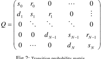
Birth-death processes are Markov chains where transitions are allowed only between neighboring states. We treat the continuous time case here, but analogous results for discrete-time case are easily obtained. A one-dimensional birth-death process is shown Fig.1 and its transition matrix is shown as:
N N
N N N
s
d
r
s
d
r
s
d
r
s
Q
0
0
0
0
0
0
0
0
0
1 1 1
1 1 1
0 0
Fig 2: Transition probability matrix
The transition rates
r
k,k
0
are state dependentbirth rates and dk,
k
1
, are referred to as state dependentdeath rates. In the limiting case when k= 0 we have
r
0
p
,1
0
s
, andd
0
0
. Similarly, for k = N we have,
0
N
r
s
N
p
,
andd
N
1
p
. The transition ratesr
k,0
k
are state dependent birth rates and dk,k
1
, arereferred to as state dependent death rates.
B. Closed-Form Solution
We now derive a closed-form solution for the Markov model derived in the previous section. Let
u
kbe the steady-state probability of being in state k, we basically compute for each possible state k the probabilityu
k. As the very first step, we write the following fixed point equation [6] for the Markov chain in Fig.1. :, 1 1 1
1
k k k k k kk
r
u
s
u
d
u
u
(1)Which expresses the steady-state probability
u
k (of being in state k) as the union of three events: (i) reaching (birth) state k from state k-1, with probabilityr
k1u
k1,
(ii) remaining instate k with probability
s
ku
k;
(iii) reaching state k from k+1,with probability
d
k1u
k1,by means of a deletion (death)event. We can rewrite the same equation as:
A. Ghaddar et al / (IJCSIT) International Journal of Computer Science and Information Technologies, Vol. 2 (6) , 2011, 2632-2636.
2633 A. Ghaddar et al / (IJCSIT) International Journal of Computer Science and Information Technologies, Vol. 2 (6) , 2011, 2632-2636.
, 1 1 1 1
)
(
r
k
d
ku
k
r
ku
k
d
ku
k (2)Which equates the probability of leaving state k, computed as
k k
k
d
u
r
)
(
to the probability of entering state k, computedas
r
k1u
k1
d
k1u
k1.
By replacingd
k1,
d
k,
r
k,
andr
k1with the actual values we obtain (3):
1 11
)
1
(
1
1
1
N
k
-1
p
k k ku
N
k
p
u
N
k
p
u
p
N
k
Where p is the probability of delay on single trial, N is the total number of independent trials (or, equivalently, the maximum number of cell-time delays). Equation 3 is a second order difference equation whose parameters are dependent on k, i.e., on the current state. We use Equation 3 and the condition for a probability distribution:
1
0
N k k ku
(4)To derive the following closed-form equation for
probability
u
k:k N k
k p p
k N
u
(1 ) (5)
The equation shows that the constant probability of birth p with a linear increasing probability of death k/N, results in a binomial distribution with mean
N
.
p
and variance)
1
(
.
p
p
N
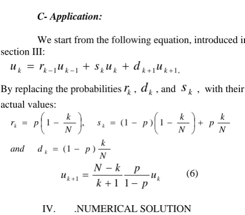
.C- Application:
We start from the following equation, introduced in section III:
u
k
r
k1u
k1
s
ku
k
d
k1u
k1,By replacing the probabilities
r
k,d
k, ands
k , with their actual values: N k p d and N k p N k p s N k p r k k k ) 1 ( 1 ) 1 ( , 1 k k u p p k k N u 1 11 (6)
IV. .NUMERICAL SOLUTION
A discrete time Markov model is defined in terms of a set of transition probabilities between the discrete states of the model. Transitions are associated with transition probabilities between states. The NxN transition probabilities between N states are called the transition probability matrix Q. If Q0 is
initial probability vector then the state probability after k steps
is given by the vector:
u
k
Q
0*
Q
k, the matrixQ
k is the k-th transition matrix after multiplying Q by itself, k times. The steady state probability vector in all states of the Markov model is such that:u
k*
Q
u
k.This equation will be used along with the condition:
N k ku
01
. In order to determine all the steady statesprobabilities for the network models [5, 9, 10].
To validate the proposed Markov chain for ATM Networks, we perform two sets of experiments. In the first set experiments, we apply a numerical solution [7, 8, 9] using Gradient Conjugate Method. For each experiment, we collect the statistics regarding the size number of steady states (N), and compare the Binomial distribution of steady states with the model distribution provided by equation 5.
We applied three different sizes, N = 500, N = 1000, and
N =1500 with the probability of delay on single trial
32
1
p
,(Fig.3, 4 and 5) for our model we assume that the ATM Network. Figure 6 shows curve of mean probability versus the number of states (2200). It can be observed that this mean probability decreases as the number of states increasing. Figure 7 shows for three numbers of states (500, 1000 and 1500) the mean probability. Also, this mean probability decreasing as the total number of states increasing.
The results we reported so far show that our model for ATM Networks in Markov Chain can predict the Binomial distribution and showed that the steady-state probability. To test whether the steady-state probability distribution of the numerical solution data is actually fits the theoretical distribution (Fig. 3, 4 and 5) provided by the model we employ the goodness of fit for discrete distributions. In all the experiments reported the Numerical solution data are compatible with a Binomial distribution, the error between numerical and analytical solutions is less than 1.E-6 for N = 500, 1000 and 1500.
To summarize, it is relatively easy for the network to extract the global properties from the total number of states N, the
probability of delay on single trial p, the birth rates
r
k anddeath rates
d
k .V. CONCLUSIONS
A. Ghaddar et al / (IJCSIT) International Journal of Computer Science and Information Technologies, Vol. 2 (6) , 2011, 2632-2636.
2635 A. Ghaddar et al / (IJCSIT) International Journal of Computer Science and Information Technologies, Vol. 2 (6) , 2011, 2632-2636.
As a conclusion, we assume that the results reported in this paper can be used in the design of computer networks systems. The analysis includes, indeed, the qualitative evaluation of the performance, and quantitative analysis consisting of the steady-state probability distribution of the Markov chain. We observe that if we apply more analysis, the results can lead to a new model. This model could simulate temporal variations on the inherent delays. Such work requires more mathematical and statistical modeling efforts.
The performance of ATM Networks is evaluated analytically and via numerical simulations. The simulations were performed on the Unix C++ programming language.
VI. FUTURE WORKS
Out of the results of the present work, some recommendations for future works are proposed:
1. Apply iterative method to evaluate network by Markov Chain as Nonstationary iterative methods such as (BiConjugate Gradient (BiCG), BiConjugate Gradient Stabilized Method, Conjugate Gradient Squared Method, and Conjugate Gradient for parallelism [7].
2. Comparison between stationary iterative methods and Nonstationary iterative methods.
3. Apply parallel Computing for very large models.
REFERENCES
[1] Robert W. Dmitroca, Susan G. Gibson, Trevor R. Hill, Luisa Mola Morales, and Chong Tean Ong. Emulating ATM Network Impairments in the Laboratory. April 1997 Hewllett-Packard Journal, Article 9. [2] Queueing Networks and Markov Chains Modeling and performance
evaluation with computer science applications, G. Bolch, S. Greiner, H. de Meer, and K. Trivedi. A wiley-Interscience publication, John Wiley & Sons. INC.
[3] Sahner R., Trivedi K., and Puliafito A., Performance and Reliability Analysis of Computer Systems – An Example-Based Approach Using the SHARPE Software Package. Kluwer Academic Publishers, Bosten, M.A., 1996.
[4] JIa Liu,Shunxiang Li, and Shusheng Jia, A Prediction Model Based on Neural Network and Fuzzy Markov Chain, IEEE 978-4244-2114-5,2008.
[5] Evaluation of the Markov Models in Computer Networks Simulation, N. Sinno, H. Youssef, and A. Ghaddar, IAENG Transactions on Engineering Technologies – Volume 4, edited by S.-I. Ao, 2010 American Institute of Physics 978-0-7354-0794-7/10/$30.00
[6] D. G. Luenberger. Introduction to dynamic systems: Theory, Models, and applications. John wiley & Sons, NY, USA, May 1979.
[7] Iterative Methods for Sparse Linear Systems, Yousef Saad, copyright©2000 Yousef Saad. Second Edition with corrections. January 3RD,2000.
[8] M. Prandini and J. Hu, “A numerical approximation scheme for reach ability analysis of stochastic hybrid systems with state-dependent switching”, in In Proc, IEEE Int. Conf. Decision and control, New Orleans, LA, Dec. 2007,pp. 4662-4667.
[9] H. J. Kushner, Approximation and Weak Convergence Methods for Random Processes with Applications to Stochastic Systems Theory. Cambridge, Massachussets: MIT Press, 1984.
[10] M. Kwiatkowska, G. Norman, and D. Parker, “Prism: Probabilistic model checking for performance and reliability analysis”, ACM SIG-METRICS performance Evaluation Review, 2009.
.
Ahmad Ghaddar received a Dipl. Ing. In 1986 from the ESICA (École Nationale Supérieure d’Ingénieurs de Constructions Aéronautiques de Toulouse – France), and in 1992 he received a Ph.D. degrees in mechanics from the university of Lille – France. He joined the department of applied mathematics at the Lebanese University. His research interests include modeling problem in mechanics, simulation computer networks, and Markov Chain.
Yasser Mohanna received his BE degree in electrical engineering from the American University of Beirut (AUB) in 1986 and his Masters and Ph.D. degrees in Optoelectronics from the National Polytechnic Institute of Grenoble (I.N.P.G.) France in 1987 and 1989 respectively. His Ph.D. and masters research work was completely done at ALCATEL FIBER OPTICS France.
He is a professor of electronics engineering at the Lebanese University (L.U.), Beirut, Lebanon. He joined L.U. in 1994 and contributed to the development of its Electronics B.S. and Masters programs. From 1992 to 1994 he was with the Liban Cables, Lebanon where he chaired the electronics section. From 1989 to 1991 he was with AOIP instrumentation France where he contributed to the design of infrared pyrometers.
Prof. Mohanna is a member of the Lebanese order of engineers. His actual fields of interest are Digital signal and image processing and processors, control systems.
Mohamed Dbouk is a full time Associate Professor at the Lebanese University (Beirut) where he coordinates a master-2 research degree “M2R-SI: Information System”. He received his PhD from Paris-Sud, France, 1997. His research interests include software engineering and information systems, geographic information systems, data-warehousing and data-mining.