Volume 2, No. 5, Sept-Oct 2011
International Journal of Advanced Research in Computer Science
RESEARCH PAPER
Available Online at www.ijarcs.info
286
ISSN No. 0976-5697
High Speed & Highly Secured Image Annotation Using Soft and Hard Watermarks
Prof. YashKshirsagar
Professor,
Department of Electronics and Communication TIT, Bhopal
Anup.V. Kalaskar*
M.Tech Student,
Department of Electronics and Communication, TIT, Bhopal
Shilpa.R.Jadhav
M.Tech Student,
Department of Electronics and Communication TIT, Bhopal
Abstract – In this paper we introduce effective data hiding for image annotation, High fidelity is a demanding requirement for data hiding for images with artistic or medical value. This correspondence proposes image watermarking for annotation with robustness to moderate distortion. To achieve the high fidelity of the embedded image, the model is built by mixing the outputs from entropy and a differential localized standard deviation filter. The mixture is then low-pass filtered and normalized to provide a model that produces substantially better perceptual hi-fidelity than existing tools of similar complexity. The model is built by embedding two basic watermarks: a pilot watermark that locate the existence of the watermark and an information watermark that carries a payload of several dozen bits. The objective is to embed 32 bits of metadata into a single image in such a way that it is robust to JPEG compression and cropping.
Keywords- Hard Watermark (HW), Soft Watermark (SW), Lapped Bi-orthogonal Transform (LBT), Mean-Squared Error (MSE), Normalized Cross-Correlation (NCC).
I. INTRODUCTION
The proposed model combines the outputs of two simple filters: entropy and a differential standard deviation filter to estimate visual sensitivity to noise. The two outputs are mixed using a non-linear function and a smoothing low-pass filter in a post-processing step. In this paper, we focus on the latter one with an objective to create a tool that annotates images with 32 bits of meta-data. Note that we do not impose any security requirements for the watermarking technology[4]. The developed watermarking technology embeds two watermarks, a strong direct-sequence spread spectrum (SS) watermark tiled over the image in the lapped bi-orthogonal transform (LBT) domain [5].
This watermark only signals the existence of the meta-data. Next, we embed the meta-data bits using a regional statistic quantization method. The quantization noise is optimized to improve the strength of the SS watermark while obeying theconstraints imposed by the perceptual model. We establish the model in the pixel domain for two reasons. First, it can be applied at no transformation cost in applications that require image transforms such as wavelets, lapped transforms, or DCT. Second, it is difficult to model perceptual quality for block transforms such as JPEG’s 8 × 8 DCT, as the assessment procedure has to have an understanding of the block interleaving (if any) as well as access to data in the neighboring blocks. In such a setup, it is difficult to predict artifacts like blocking, aliasing, ringing along edges etc. Note that the objective is different with respect to previous models as it aims at quantifying a “bound” on the perceptually “invisible” additive noise as opposed to quantifying how perceptually
similar two images are.
The related work on visual models has focused on establishing a function over the visual features of two images to establish how similar they are, or how closely they appeal to the human eyes. While simple heuristics such as mean-squared error (MSE) and peak signal-to-noise ratio (PSNR) are easy to compute and integrate in optimization scenarios, they have been abandoned long ago for high-quality image quality assessment [1]. On the other hand, novel sophisticated models have been mainly focusing on combining feature statistics. An excellent survey of related work prior to year 2009 is given in [2], and a review of most recent work including a novel visual fidelity assessment methodology is reviewed in [3]. In this paper, we tryto provide a solution to the following problem:given an image I ∈ {Z∗}m×n find a function f() : Z∗}m×n → {Z∗}m×n whose result f(I) quantifies pixel-wise the magnitude of random noise In that one can add to I so that the resulting image I + In is perceived as a high quality copy of I.
II. NOISE TOLERANCE OF MODEL
S(k,r)= (1)
E(k,r) = - (2)
p(k, i) = Pr[k = i|k∈Π(k)]. (3)
The entropy map E (k, r) indicates the complexity of the neighborhood for a given pixel. This is a simple heuristic to identify pixels that are perceptually less tolerant to noise. Empirically, this claim usually holds true for pixels with low E (k, r), i.e., regions with smoothly changing luminosity. It is important to stress that high value of E (k, r) does not necessarily imply strong tolerance to noise. we use a differential standard deviation filter D (k) = |S (k, r1) − S (k, r2 )|, r1> r2 , to expose the effect of edges on visual fidelity. If both S (k, r1) and S (k, r2) are low, then we intuitively conclude that the r1-neighborhood centered on k is not tolerant to noise similarly to the entropy filter. On the other hand, if both S (k, r1 ) and S (k, r2 ) have high values, one can certainly assume that the visual content around k is noisy and that it more noise-tolerant. The interesting case occurs for disproportionate S (k, r1) and S (k, r2); in most cases this signals an edge in the neighborhood of k and low tolerance to noise. In order to reflect these phenomena we empirically selected D( ) as a fast, In order to mix the E( ) and D( ) features, we first normalize both feature matrices and then combine them as follows:
m(D,E) = exp (4)
The mixing function is non-linear and has the shape of a 2D Gaussian distribution, where parameter s adjusts the shape of the function. In Fig1 it resembles a smooth AND operator between E and D. Low values of s raise the complexity value for the pixel with both high E and D while suppressing other pixels. Large s allows pixels with moderate E and D to have moderately high complexity value.
We finalize the process by filtering D(k) with a 3 ×3 spike
filter:
F1={ } (5)
followed by a low-pass filter to obtain m’(D, E). This processing aims at exposing only strong edge effects. Finally, by scaling m(D, E)/m’(D, E) and then normalizing the result, we create the final complexity map f(I).
Figure1. Block diagram of the processing involved in computing a complexity map for a given image.
III. CONCEPTIONANDEMBEDDING OF SOFT&
HARD WATERMARK
The objective is to embed 32 bits of meta-data as a hard watermark into an image so that their detection is as robust
watermarking schemes that pertain to this goal, can use the developed visual model to achieve visual transparency as well.
We built the system in two steps: first, we embed a soft, spread-spectrum watermark whose objective is to signal metadata presence. If this watermark is detected, the decoder proceeds with the message extraction by analyzing localized statistics of the image. Here we overview the two techniques.
A. Soft Watermark:
The soft watermark (SW) serves two purposes:
a. To detect the existence of the meta-data, b. To enable image registration at the detector side due to potential cropping or other type of misalignment.
We design the Soft Watermark (SW) to be a random i.i.d. sequence taking value from {-1, 1} or drawn from a standard normal distribution N(0, 1). The SW is spread over a continuous image region of size L.
We denote this region the basic SW block. We create a full image watermark by tiling the same basic SW block. Consequently, the smallest image that can be augmented with meta-data is the size of the basic SW block. In order to reduce blocking effects, we propose to embed the SW in the Lapped Bi-orthogonal Transform (LBT) domain [5]. In the LBT domain, we choose to leave the DC and high frequency components untouched for better visual quality and robustness to lossycompression,respectively. We introduce a mask for each 4-by-4 block of the LBT image:
t = (6)
where ones indicate the LBT coefficients used for SW embedding. Next, we use f(I) to adjust the energy of the SW according to the content of the image. Since the complexity map is in the pixel domain, we take the inverse LBT transformation of the watermarked image and re-weight the watermark in the pixel domain using f(I). With the above considerations, the SW embedding can be expressed as:
Y = I+αf(I){LBT−1[LBT(I)+wt]−I} (7)
where wt denotes the masked SW, and Y represents the watermarked image. Parameter a adjusts the watermark energy to achieve the desired trade-off between visual
quality and robustness. In our experiments, we used α = 10
in order to create images within 55-50dB PSNR from the original. The SW alone is hardly visible at these noise levels. However, it conveys only one and halfbits of information to the detector.
B. Hard Watermark:
The hard watermark (HW), which represents the meta-data bits.Here we enter 32 bit wide hard watermark.
[x y z ...]: [1 1 0 0 1 1 0 0 1 1 0 0 1 1 0 0 1 1 0 0 1 1 0 0 1 1 0 0 1 1 0 0]
288
k = (8)
where K is denoted as the scaling constant. Typically, we aim at K such that the size of the building block is between 4 ×4 and 8 × 8 pixels. For example, for a basic SW block of size 640 × 480, and K = 48, e.g., a building block of dimensions 8 × 6 pixels, we obtain K = 200. Then, for each meta-data bit, we randomly assign exactly K distinct building blocks within the pixel field of the basic SW block. We denote the set of all coefficients that belong to these building blocks as Ai, I = 1 . . . 32.
We compute the first order statistics of the coefficients in each Ai:
(9)
To embed a bit b1, we quantize µto an even number of Qs if b1has value 0, or to an odd number of Qs ifits value is one. Here, Q is the quantization step size. That’s:
µ’I = (10)
∆µi = µ’i- µi (11)
Where µ’iis the mean value after HW embedding and
∆µiis the corresponding Ai-wide change. It is straightforward to notice that larger Q results in a more robust HW at the cost of decreased visual quality.
The next step is to adjust the pixel values in also that the changes of its mean value equal ∆µi . To get better visual quality, we deploy f (I) to allocate and quantify the HW for each pixel. We design the change of each pixel value, y (p), p ∈ Ai, to be proportional to its complexity value f (p):
∆y(p) = ∆µikK (12)
where ∆µikK corresponds to the total changes of the pixel values inside Ai. For certain images, the building blocks in Aimay consist of only smooth regions. Then, large
∆µwill result in a large change for most of the pixels in
Aand likely incur visual distortion. To provide high-fidelity,
we first examine the summation of the complexity values in
Aiand compare it with a threshold hcto decide whether Aiis suitable for embedding or not. If the complexity of Aiis high enough, we apply the above mentioned embedding otherwise we discard the block and discard the bit. Parameter hccan be chosen to trade off the robustness of the HW and visual quality. Since the building blocks in Aiare chosen randomly, the probability for the complexity of Ai below threshold hcis usually very low. In all of the conducted experiments, all image blocks were complex enough for embedding. The above hard watermark embedding does not take into account the SW that has already been embedded in the image. Since the allocation of watermark energy to individual pixels has a lot of freedom, we can reallocate the watermark in a way that favors the SW detection while maintaining the accuracy of the HW detection.The objective is to allocate the HW to pixels so that the correlation of the watermarked image with SW becomes higher. This can be done by choosing only the pixels whose corresponding SW component has the same sign as the ∆µifor embedding:
∆y(p) = ∆µikK
0 otherwise (13) A’I = {p|sign(SW(p)) = sign(∆µi), p Ai}.
In our experiments on a database of over 41 large images,after embedding both the soft and hard watermark,
we have observed a resulting PSNR in the range from 49-40dB.
ORIGNAL IMAGE
ANNOTATED IMAGE
Figure.2. Demonstration of the visual differences between the original image with no watermark, and annotated image with both soft and hard watermarks augmented. The annotated image illustrate the actual pixel value alterations after embedding the both the watermarks.
IV. WATERMARK EXPOSURE
The detection process consists of two steps. First, we determine whether the test image contains a SW. If yes, we move on to extract the embedded meta-data.
A. Soft Watermark Detection:
c(zi, w) = (14)
for each sub-block zi∈z'. Operator ā denotes the mean of the argument a. Fast NCC for image registration can be computed via the FFT. Image z is declared tainted with w if max [c(z, w)] > T , where T is the detection threshold that identifies the probability of a false positive or negative according to the gaussian error function. In our case, we
compute the standard deviation σ over (∀zi∈ z’) c (zi, w) and determine T such that probability of a false negative is:
F N = (15)
where W denotes the cardinality of the SW. Once the SW is detected, the detector can identify its location in the image and therefore the location of the meta-data.
B. Hard Watermark Detection:
The extraction of the meta-data is rather simple. First, thedetector identifies the building blocks corresponding to each bit. Then, the mean pixel value ˆµ’iover each set of building blocks is calculated. The bit is extracted by quantizing ˆµ’iusing Q, and examining whether the quantized value is odd or even.
(16)
Wherebiis the extracted bit, In case when there exists more than one SW, the detector uses a soft decoding technique. For simplicity, we use a repetition code to encode each metadata bit, i.e., we augment each bit in each basic SW block separately. We denote asthe bitb(r, i) the i-th extracted copy offrom the r-th basic SW block. For each bit, we record the distance d(r, i) of the statistic µ’ito nearest reconstruction point. This value quantifies the confidence level of the detection for each raw bit. We collect this soft information for all extracted bits & estimate the final metadata bit Bibased on the confidence scores S0and S1:
Bi = (17)
Sx =
V. EXTRA WORK
We aim at a simple ad-hoc approach that empirically shows balance between speed and simplicity of computation and accuracy in quantifying perceptual tolerance to noise.
Besides already mentioned surveys, image assessment work has been reviewed and benchmarked in [8]. Standard techniques such as MSE and PSNR have not been matched well to perceived visual quality [1]. Some of the main trends in the field are at the intersection between cognitive sciences [9], understanding the workings of the visual cortex, and ad-hoc heuristics. For example, one class of algorithms separates images into sub-bands (i.e., channels) that are selective for spatial and temporal frequency and orientation. Sophisticated channel decompositions analyze the neural responses in the primary visual cortex [10], [11], [12].
Alternatively, many metrics use simpler transforms such as the DCT [13] or separable wavelet transforms [14], [15] to achieve the same goal. Channel decompositions based upon temporal frequencies have also been used for video quality assessment [16].
One of the most difficult aspects of the problem is its definition [17]. once resolved, analytical progress is likely to follow rapidly. For example, certain distortions may be
visible but not considered of poor fidelity suggesting that correlation between image fidelity and visual quality is arguable [1], [18]. One approach is to combine several visual models typically mixed using the Minkowski norm, which inherently assumes spatial independence [19]. Thus, visual masking models have been proposed to account for the interdependence of image coefficients [10].
VI. RESULTS
We have done maximum possible experiments to prove our proposed method and finally we got effective results for efficient image annotation in which we hide 32 bit meta-data in any high fidelity image with medical or any precious value for which used HW and SW. While doing all this we embed:
32 bit wide hard watermark
[x y z ...]:[1 1 0 0 1 0 1 1 0 1 1 0 0 0 0 0 0 0 1 1 1 1 1 1 1 1 1 1 1 1 1 0]
For which the First Order statistics is:
Table I: First Order statistics is:
Columns 1 To 446.3594 463.9707 442.4766 341.7617
After embedding the given 32 bit wide hard watermark there is shifting in the first order statistics:
Table II: The Shifted First Order Statistics
Columns 1 To 389.2480 453.4023 439.0723 405.2949
0 0 0 0
The difference of order first order and shifted order statistics is used to evaluate the difference order statistics:
Table III: Differential Order Statistics
Columns 1 To 410.3477 458.8691 447.7930 378.4785
0 0 0 0
0 0 0 0
420.5156 457.6406 454.3574 352.3301 446.3594 463.9707 442.4766 341.7617
290
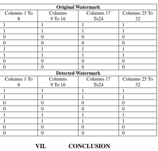
Table IV: comparison of the embedded Watermark and detected water mark
Original Watermark Columns 1 To
8
Columns 9 To 16
Columns 17 To24
Columns 25 To 32
1 1 1 1
1 1 1 1
0 0 0 0
0 0 0 0
1 1 1 1
1 1 1 1
0 0 0 0
0 0 0 0
Detected Watermark Columns 1 To
8
Columns 9 To 16
Columns 17 To24
Columns 25 To 32
1 1 1 1
1 1 1 1
0 0 0 0
0 0 0 0
1 1 1 1
1 1 1 1
0 0 0 0
0 0 0 0
VII. CONCLUSION
We have conducted several experiments to evaluate our proposed method on a database of 41 challenging images. Figure 1 shows a small portion of one of the original test images with a large smooth region. Most of the semantic content of the image is expressed as an edge. This is an example of an image which is relatively hard to watermark in-perceptively. The same figure illustrates the output of an existing hi-fidelity watermarking scheme compared to our result. The two schemes have approximately the same maximal luminosity noise, however, the overall PSNR in the Y-channel is 42dB vs. 38dB for our vs. the existing proposal respectively. Both the soft and the hard watermark survive a JPEG compression with the quality parameter set to 30 and with €FN= confidence.
VIII. REFERENCES
[1]. B. Girod, “Whats wrong with mean-squared error,” Digital Images and Human Vision, MIT Press, pp.207-220, 1993.
[2]. Shan He; Kirovski, D. Min Wu; Thomson Corp. Res., Princeton, NJ, “A Novel Visual Perceptual Model with AnApplication to Hi-Fidelity Image Annotation, IEEE Trans. Image Processing,vol.18,pp.429–434, 2009.
[3]. Z. Wang, et al., “Image quality assessment: From error visibility to structural similarity,” IEEE Trans. on Image Processing, vol.13, no.4, pp.600–612, 2004.
[4]. I.J. Cox, et al., “A secure, robust watermark for multimedia,” Info Hiding Workshop, pp.183–206, 1996.
[5]. H.S.Malvar, “Biorthogonal and Nonuniform Lapped Transforms for Transform Coding with Reduced Blocking and Ringing Artifacts,” IEEE Trans. on Signal Processing, pp.1043–1053, 1998.
[6]. P.C.Teo&D.Heeger,“Perceptual image
distortion,SPIE,vol.2179, pp.127-141, 1994.
[7]. J. Lubin, “A visual discrimination model for imaging system design and evaluation,” in Visual Models for Target Detection and Recognition, World Scientific, pp.245-283, 1995.
[8]. S. Daly, “The visible differences predictor: An algorithm for the assessment of image fidelity,” Digital Images and Human Vision, pp.179206,MIT Press, 1993.
[9]. Z. Wang, et al., “Why is image quality assessment so difficult,” IEEE ICASSP, vol.4, pp.3313-3316, 2002.
[10].D.A. Silverstein and J.E. Farrell, “The relationship between image fidelity and image quality,” IEEE ICIP, pp.881-884, 1996.