Design and Development of Grey Wolf Optimization Algorithm to Solve Economic Dispatch Problem

(1)

ISSN (Print) : 2320 – 3765 ISSN (Online): 2278 – 8875

I

nternational

J

ournal of

A

dvanced

R

esearch in

E

lectrical,

E

lectronics and

I

nstrumentation

E

ngineering

(A High Impact Factor, Monthly, Peer Reviewed Journal)

Website: www.ijareeie.com

Vol. 7, Issue 3, March 2018

Design and Development of Grey Wolf

Optimization Algorithm to Solve Economic

Dispatch Problem

Sangeetha.S1, Elango.M.K2

P.G. Student, Dept. of EEE, K.S.Rangasamy College of Technology, Tiruchengode, Tamilnadu, India1

Professor, Dept. of EEE, K.S.Rangasamy College of Technology, Tiruchengode, Tamilnadu, India2

ABSTRACT: With a specific ultimate objective to take care of economic dispatch issue in a helpful way, GWO algorithm is actualized in this paper. The conservative dispatch intends to locate the aggregate power generation of different units in a plant at least cost. This paper, for the most part, intends to limit the aggregate cost of power generation by utilizing GWO algorithm. In the meantime, this algorithm is focused on enhancing the effectiveness of power generation and it is focused on taking care of the power demand. The monetary dispatch issue is a vital streamlining issue in scheduling the generation of thermal generators in power system. The proposed procedure is executed on IEEE standard six unit and fifteen unit test frameworks. The acquired outcome by utilizing this algorithm is contrasted with PSO-ANFIS technique has been finished. The outcomes inform the highness of GWO algorithm among different strategies to take care of economic dispatch issue.

KEYWORDS: Economic dispatch problem; quadratic cost function; prohibited operating zones; ramp rate limit; valve point effect; grey wolf optimization

I.INTRODUCTION

(2)

I

nternational

J

ournal of

A

dvanced

R

esearch in

E

lectrical,

E

lectronics and

I

nstrumentation

E

ngineering

PSO technique, the conventional PSO is modified such as Hybrid PSO (HPSO), PSO-ANFIS [5] and Gaussian and Chaotic PSO [6]. Nowadays, number of various optimization techniques is proposed to solve the economic load dispatch problem. They are named as Chaotic Ant Swarm Optimization (CASO), Bacteria Foraging Optimization (BFO), Ant Colony Optimization (ACO), Gravitational Search Algorithm (GSA) and Biogeography Based Optimization (BBO). These techniques are able to provide an efficient solution but it does not obtain fast convergence rate and it has several parameter tunings.

In this paper, GWO [7] algorithm has been used which is a powerful and newly emerged technique. This technique is inspired by the grey wolves. It mimics the leadership hierarchy and hunting mechanism of grey wolves. This technique has successfully applied in various power systems optimization problems, recently. It can highly improve the converging speed and obtain an optimal solution easily. The GWO algorithm is the best conveying mechanism and it considers three candidate solutions randomly to get better results. It converges quickly by jumping from local optimal solution towards a global optimal solution. The proposed GWO approach is applied to solve IEEE six unit and 15 unit test systems to justify the effectiveness of this method. The performance of this solution results is compared with PSO-ANFIS technique.

II. ECONOMIC DISPATCH PROBLEM FORMULATION

In power system, the economic load dispatch is one of the most important optimization problems. The following objective and constraints are taken into consideration in the formulation of economic load dispatch problem.

A. The Objective Function

The objective of economic load dispatch is to minimize the total fuel cost in power generation while satisfying all the equality and inequality constraints. The following equation represents a simple formulation of economic load dispatch problem.

= ∑ ( ) (1)

Subject to,

≤ ≤ (2)

∑ = + (3)

where Fi (Pgi) is the fuel cost function of generating unit i, Pgiis the power output of generating unit i, PD is the power

demand, Pgimin and Pgimaxare the lower and upper limits of generating unit i and PL is the total system loss.

B. Quadratic Cost Function

The total fuel cost function is expressed as the sum of a quadratic function. The function is represented as

∑ ( ) =∑ ( ) + ( ) + (4)

where ai , bi and ci are the total fuel cost coefficients for generating unit i

C. Cost Function with Valve-Point Effect

In the generating units, the real input-output cost curves are non-convex due to valve point effect. A half tide resultant is generated in the steam entrance through the valve in a turbine, so it is more practical for considering the valve point effect with fuel cost function to affix flexible operational facilities. The fuel cost function in terms of real output power can be represented as the sum of a quadratic function and sinusoidal function in the following equation.

(3)

I

nternational

J

ournal of

A

dvanced

R

esearch in

E

lectrical,

E

lectronics and

I

nstrumentation

E

ngineering

D. Constraints

Constraints in generator are considered as following.

1) Generator Capacity Constraints: The output power of each generating unit should be less than or equal to the

maximum power permitted and also be greater than or equal to the minimum power permitted on specified unit. It can

be written as

≤ ≤

2) Power Balance Constraints: The total output power is generated by the generating units should be equal to the

sum of power demand and transmission loss. It is mathematically expressed as

= +

PLis the transmissionloss and it is calculated by using Kron’s loss formula or the B coefficient formula, as follows:

=∑ ∑ +∑ + (6)

where B , B0 and B00 are the loss coefficients.

3) Prohibited Operating Zones: Due to the presence of physical operations such as vibration in shift bearing,

some faults in generating units or their accessories like boiler and feed pumps, the generating units might have

prohibited operating zones in an input-output curve of the generator. The generating units should avoid the operation in

prohibited zones. It can be formulated as follows.

≤ ≤ , (i=1,2,...,n)

, ≤ ≤ , (j=2,3,..ni-1)(i=1,2,..,n)

, ≤ ≤ (i=1,2,...,n) (7)

where Pgi,1 is the lower bound of a jth prohibited operating zone of generating unit i, Pgi,j is the upper bound of a jth

prohibited operating zone of generating unit i, nj is the total number of prohibited operating zones of generating unit i.

4) Ramp Rate Constraints: The successful operation of generating unit’s range is prohibited by its ramp rate

limit. In actual systems, the output power of generating units cannot change suddenly. The changes in output power

occur from one specific interval to the next cannot exceed a specified limit. It can be expressed by following equations.

As the output power increases,

− ≤ (8)

As the output power increases,

− ≤ (9)

Combining (8) and (9) with (2) can be written as,

(4)

I

nternational

J

ournal of

A

dvanced

R

esearch in

E

lectrical,

E

lectronics and

I

nstrumentation

E

ngineering

where Pgi0 is the unit output power at a previous interval, U Ri and R Ri are the up-ramp and down-ramp limits of

generating unit i.

III. GREY WOLF OPTIMIZATION ALGORITHM

A. GWO Algorithm

GWO algorithm is an optimization method which is presented newly. It is inspired by the wolves of grey. It has the hierarchy of leadership and mechanism of hunting in grey wolves. The grey wolves are divided into four types and that wolves form a group. It is represented in a hierarchical system in the form of alpha (α), beta (β), delta (δ) and omega (ω). From the hierarchy of leadership system, the leader can be either a male or a female called alpha. It takes the power to make a verdict for hunting, place to sleep etc..,. The next to alpha, beta is the ancillary wolf that helps to alpha for taking a decision. The next to beta, delta is the third level of the hierarchical system which dominates the omega. The lowest order of grey wolves in the hierarchical system is omega. It should ever pursue the discipline of α, β and δ.

B. Model of GWO

Developing the model which is based on social hierarchy and hunting mechanism of GWO.

1) Social Hierarchy: The main three wolves (α, β & δ) are considered to find the fitness solution. The remaining

wolves (ω) follow the instruction of main wolves.

2) Encircling Prey Wolves are going to hunt for prey. They surround the prey when they locate the prey where it

is. Sorrounding the prey by grey wolves is modeled by equations (11) and (12).

= | . ( )− . ( )| (11)

( + 1) = ( )− . (12)

where the present iteration is denoted as t, the preys position vector is represented as Vp, the grey wolves position vector are represented as V and the coefficient vectors are named as A & C. The coefficient vectors are determined by the equations (13) and (14).

= 2 . . (13)

= 2. (14)

where the component of a is decreased gradually in each and every iteration from the value 2 to 0 and the random variables are denoted as r1and r2 which are in the interval [0,1]. The position of grey wolves is updated in each and

every iteration to attain the best optimal solution by utilizing the equations (11) and (12).

3) Hunting for Prey: The ultimate job of grey wolves is hunting process. The wolves are involved in hunting for

getting their prey. At first, they cannot locate the prey where itis but they have to find the location of prey. Among all wolves, alpha takes the lead role to guide all other wolves. Beta and delta helps to alpha for making decision. Finally, the grey wolves with the guidance of main wolves achieve the location of prey i.e., the best optimal solution. These all are modeled by using equations (15), (16) and (17). The three best solutions are carried out in entire process. For that, the position of grey wolves is updated over every iterations.

= | . − |

= | . − | (15)

= − .

= − . (16)

(5)

I

nternational

J

ournal of

A

dvanced

R

esearch in

E

lectrical,

E

lectronics and

I

nstrumentation

E

ngineering

Here, the positions of grey wolves i.e., the three best solutions are represented as Vα, Vβ& Vδ. The location of prey is

examined by the main three wolves of α, β and δand the remaining wolves are surrounded the prey by the instruction of alpha.

4) Attacking Prey: The grey wolves attack the prey when they find the location of prey. The preys are stopped to

move at one situation. At that time, the grey wolves easily attack the prey and they had it. This is the termination of hunting process of grey wolves. The situation to attack the prey is made by the value of coefficient vector A. It is in an interval [-2a, 2a]. The value of a is reduced linearly from 2 to 0. When |A| < 1, the wolves are moved over prey to attack. This is the condition of grey wolf to attack the prey. The position of grey wolves is updated to find the best three solutions.

5) Searching Prey: Initially, the wolves cannot locate the place of prey in hunting process. So, they started to search for locating the prey. All wolves are not gone in same direction. They are separated from each other for finding the location of prey. When they locate the prey, the wolves are joined back together and start to attack it. The whole process is smoothly led by alpha, the best solution. The equation (13) can be given an instruction to wolves for diverging from each other. When |A| > 1, the prey is attacked by wolves and finally it brings the ending in process of hunting.

The following synopsis defines the Grey Wolf Optimization (GWO) algorithm.

1. Initialize the number of grey wolves is involved in whole process i.e., the size of population is initialized. 2. And also initialize the position of grey wolves and prey which is surrounded by wolves in the random location i.e., the iteration point is fine-tuned at maximum.

3. Among all the grey wolves, finding the fitness solution is the ultimate task in at individual wolf. The fitness solution is nothing but the distance between location of prey and an individual wolf.

4. By calculating the fitness value, the three best wolves are analyzed and it is said as alpha, beta and delta. Prey’s location is identified in the hunting process by utilizing equation (15).

5. The updating positions of grey wolves are necessary to find the best solution utilizing equations (16) and (17). 6. Repeating the step 3 to step 5 until the grey wolves reach the location of prey for attacking it. The best solutions are the main three wolves.

7. The optimal solution is attained when the process reaches its terminating criterion i.e., the maximum iteration point.

IV. IMPLEMENTATION OF GWO ALGORITHM IN ECONOMIC LOAD DISPATCH PROBLEM

GWO algorithm is implemented to do the optimization in economic dispatch problem. The upcoming steps convene the implementation of GWO in economic dispatch problem.

(6)

I

nternational

J

ournal of

A

dvanced

R

esearch in

E

lectrical,

E

lectronics and

I

nstrumentation

E

ngineering

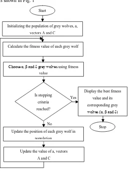
The flowchart of GWO algorithm is shown in Fig. 1

Fig. 1 Flowchart of GWO algorithm

Step 2: Initialize the parameters which are involved in GWO to solve economic dispatch problem i.e., the population size, maximum iteration point and stopping criterion.

Step 3: Initialize the design variable (B) and it is chosen by how many number is needed for the test systems. In consonance with population size, originated the design variable for test systems randomly by using equation (18).

= , + (1) × ( , − , ) (18)

where j=1,2,..,N and i=1,2,..,B. Then the formation of matrix B × N is done by utilizing equation (13).

Step 4: The best solution of fitness value is calculate in each and every individual population by using Fp. The best solution values are determined i.e., α, β and δ. The best solutions are arranged in higher order by using equation (19).

= ( ), = ( −1) = ( −2) (19)

Step 5: The design variables are identical to fitness values Fpα, Fpβand Fpδ are kept as Pα(t),Pβ(t) and Pδ(t) respectively.

Step 6: The fuel cost coefficients are evaluated by using equations (13) and (14).

Step 7: The position of individual grey wolves and prey are updated using equations (15) to (17).

Step 8: The process can be stopped when it reaches the termination criterion unless repeating the steps 4 to 7 until it reaches the terminating criterion of the GWO algorithm.

Start

Initializing the population of grey wolves, a,

vectors A and C

Calculate the fitness value of each grey wolf

Choose α, β and δ grey wolves using fitness

value

Update the value of a, vectors

A and C

Stop Yes

No

Display the best fitness

value and its

corresponding grey

wolves (α, β and δ)

Update the position of each grey wolf in

population Is stopping

criteria

(7)

I

nternational

J

ournal of

A

dvanced

R

esearch in

E

lectrical,

E

lectronics and

I

nstrumentation

E

ngineering

V. RESULTS AND DISCUSSION

A. Results

In order to show how to solve the economic load dispatch problem by using grey wolf optimization algorithm and to verify the feasibility of GWO, two practical power systems are engaged to test the algorithm. In practical power systems, the ramp rate limit and prohibited operating zones are included. The proposed GWO algorithm results are compared with PSO-ANFIS technique by two power systems of six unit and fifteen unit test systems.

System 1: The system 1 is IEEE standard six unit systems. It consists of 6 thermal units, 26 buses and 46 transmission lines. The load demand of the system is 1263 MW. The generating unit capacity and fuel cost coefficients of the six unit system are given in Table I. In the conventional operation of the system, the transmission loss coefficients B is given in Table II. The best solutions are obtained by the evolutionary process of the proposed method are shown in Table III.

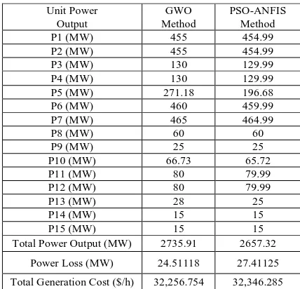
System 2: The system 2 contains 15 thermal unit systems. The load demand for this system is 2630 MW. The generating unit capacity and fuel cost coefficients of 15 unit system are given in Table IV. In this system, the loss coefficient matrix is not mentioned due to space limitation. The best solutions are obtained by the evolutionary process of the proposed method are shown in Table V.

TABLE I

Generating Unit Capacity and Fuel Cost Coefficients of 6 Unit Systems

Unit

Pimin(MW) Pimax(MW) ai bi ci

1 100 500 240 7.0 0.0070

2 50 200 200 10.0 0.0095

3 80 300 220 8.5 0.0090

4 50 150 200 11.0 0.0090

5 50 220 220 10.5 0.0080

6 50 120 190 12.0 0.0075

Table II

Loss Coefficients B of 6 Unit Systems

Bij 1 2 3 4 5 6

1 0.0017 0.0012 0.0007 -0.0001 -0.0005 -0.0002

2 0.0012 0.0014 0.0009 0.0001 -0.0006 -0.0001

3 0.0007 0.0009 0.0031 0 -0.001 -0.0006

4 -0.0001 0.0001 0 0.0024 -0.0006 -0.0008

5 -0.0005 -0.0006 -0.001 -0.0006 0.0129 -0.0002 6 -0.0002 -0.0001 -0.0006 -0.0008 -0.0002 0.0150

B0i -0.0004 -0.0001 0.0007 0.0001 0.0002 -0.0007

B00 0.056

Table III

Best Solution of 6 Unit Systems

Unit Power Output

GWO Method

PSO-ANFIS Method

P1 (MW) 450.6635 447.0687

P2 (MW) 171.0152 173.1805

P3 (MW) 268.6272 263.9225

P4 (MW) 140.7383 139.0511

P5 (MW) 166.9556 165.5761

P6 (MW) 84.0125 86.6164

Total Power Output (MW) 1282.01 1275.4153

Power Loss (MW) 12.1472 12.9584

(8)

I

nternational

J

ournal of

A

dvanced

R

esearch in

E

lectrical,

E

lectronics and

I

nstrumentation

E

ngineering

Table IV

Generating Unit Capacity and Fuel Cost Coefficients of 15 Unit Systems

Unit Pimin_(MW) _Pimax_(MW) _ai _bi _ci

1 150 455 671 10.1 0.000299

2 150 455 574 10.2 0.000183

3 20 130 374 8.8 0.001126

4 20 130 374 8.8 0.001126

5 150 470 461 10.4 0.000205

6 135 460 630 10.1 0.000301

7 135 465 548 9.8 0.000364

8 60 300 227 11.2 0.000338

9 25 162 173 11.2 0.000807

10 25 160 175 10.7 0.001203

11 20 80 186 10.2 0.003586

12 20 80 230 9.9 0.005513

13 25 85 225 13.1 0.000371

14 15 55 309 12.1 0.001929

15 15 55 323 12.4 0.004447

TABLE V

Best Solution of 15 Unit Systems

Unit Power Output GWO Method PSO-ANFIS Method

P1 (MW) 455 454.99

P2 (MW) 455 454.99

P3 (MW) 130 129.99

P4 (MW) 130 129.99

P5 (MW) 271.18 196.68

P6 (MW) 460 459.99

P7 (MW) 465 464.99

P8 (MW) 60 60

P9 (MW) 25 25

P10 (MW) 66.73 65.72

P11 (MW) 80 79.99

P12 (MW) 80 79.99

P13 (MW) 28 25

P14 (MW) 15 15

P15 (MW) 15 15

Total Power Output (MW) 2735.91 2657.32

Power Loss (MW) 24.51118 27.41125

Total Generation Cost ($/h) 32,256.754 32,346.285

B. Discussion

Table III and Table V show the best solution of 6 unit and 15 unit test systems. It gives the optimum solution of economic load dispatch problem. It generates the output power at minimum cost and it meets the load demand while power balance equation is to be maintained. The iterations are taken into account to get the best solution. The proposed method’s solution of output power and power generation rate are compared with the PSO-ANFIS technique. The output power of GWO method is greater than PSO-ANFIS technique in both test systems. The loss of power is reduced in GWO when it is compared with the PSO-ANFIS technique. The total generation cost is calculated by adding each and every unit cost of power generation. By comparing the total generation cost of GWO is with PSO-ANFIS technique, the minimum cost of power generation is attained by GWO. Therefore, GWO gives the better optimum solution to solve the economic dispatch problem than PSO-ANFIS technique.

VI. CONCLUSION

(9)

I

nternational

J

ournal of

A

dvanced

R

esearch in

E

lectrical,

E

lectronics and

I

nstrumentation

E

ngineering

system planning and operation. And also it can be tried in complex hydrothermal scheduling unit for getting good results.

REFERENCES

[1] C. E. Lin and G. L. Viviani, “Hierarchical economic dispatch for piece-wise quadratic cost functions,” IEEE Trans. Power App. Syst., vol. 3, no. 6, pp.1170-1175, Jun.1984.

[2] Moumita Pradhan, Provas Kumar Roy, Tandra Pal, “Grey wolf optimization applied to economic load dispatch problems,” Elec. Power Energy Syst., vol. 3, no. 3, pp. 325-334. Apr.2016.

[3] Wael T. Elsayed and Ehab F. El-Saadany, “A Fully Decentralized Approach for Solving the Economic Dispatch Problem,” IEEE Trans. Power Syst., vol. 30, no. 4, pp. 2179-2189. Aug.2014.

[4] S. Chakraborty, T. Senjyu, A. Yona, A. Y. Saber and T. Funabashi, “Solving economic load dispatch problem with valve-point effects using a hybrid quantum mechanics inspired particle swarm optimization,” IET Gener. Transm. Distrib., vol. 5, no. 10, pp. 1042–1052. Apr. 2011. [5] J. H. Park, Y. S. Kim, I. K. Eom and K. Y. Lee, “Economic load dispatch for piecewise quadratic cost function using Hopfield neural network,”

IEEE Trans. Power Syst., vol. 3, no. 3, pp. 1030-1038, Aug.1993.

[6] K. Y. Lee, A. Sode-Yome and J. H. Park, “Adaptive Hopfield neural network for economic load dispatch,” IEEE Trans. Power Syst., vol. 13, no. 2, pp. 519-526, May.1998.

[7] Guntas and Sushil Prashar, “Formulation of Improved Grey Wolf Optimization Methodology for EELD Problem,” Int. J. science Tech. & Eng., vol. 3, no. 3, pp. 23-31. 2016.

[8] S. Mirjalili, S. M. Mirjalili and A. Lewis A, “Grey wolf optimizer,” Adv. Eng. Soft., vol. 69, pp. 46-61, Mar.2014.

[9] El-Fergany, A. Attia and H. M. Hasanien, “Single and multi-objective optimal power flow using grey wolf optimizer and differential evolution algorithms” Elec. Power Comp. Syst., vol. 43, pp. 1548-1559, 2015.

[10] Giulio Binetti, Ali Davoudi, Frank L. Lewis, David Naso and Biagio Turchiano, “Distributed Consensus-Based Economic Dispatch With Transmission Losses,” IEEE Trans. Power Syst., vol. 29, no. 4, pp. 1711 - 1720. Jul.2014.

[11] Navneet Singh Bhangu and Gurinder Gupta, “Grey wolf optimization technique for solving economic load dispatch problem,” Int. J. Ind. Elect. & Elec. Eng., vol. 4, no. 9, pp. 133-136. Sep.2016.

[12] R. Saravanan, S. Subramanian, V. Dharmalingam and S. Ganesan, “Generation scheduling of wind thermal integrated power system using grey wolf optimization”, IOSR J. Elec & Elect Eng., vol. 11, no. 6, pp. 48-55. Dec.2016.

[13] Sudip Kumar Ghorui, Roshan Ghosh and Subhashis Maity, “Economic Load Dispatch of Power System Using Grey Wolf Optimization with Constriction Factor,” Int. J. Scientific Eng. Res., vol. 7, no. 4, pp. 320-332. Apr.2016.

[14] S. Mirjalili, S. M. Mirjalili and A. Lewis A, “Grey wolf optimizer,” Adv. Eng. Soft., vol. 69, pp. 46-61, Mar.2014.