Smooth nonparametric maximum likelihood estimation for population pharmacokinetics, with application to quinidine

SMOOTH NONPARAMETRIC MAXIMUM LIKELIHOOD ESTIMATION FOR POPULATION PHARMACOKINETICS, WITH

APPLICATION TO QUINIDINE by

Marie Davidian and A. Ronald Gallant

Institution of Statistics Mimeograph Series No. 2221

May, 1992

MIMEO Marie Davidian and SERIES A. Ronald Gallant

SMOOTH NONPARAMETRIC !

#2221 MAXIMUM LIKEIHOOD ESTIMATI~ ESTIMATION FOR POPULATION PHAR~ffi-

I

COKINETICS, WITH APPLICATION TO I

QUINIDINE ...

NAME DATE

Hit' Ubrary of

the

Depmtmeot of S'ttltis'tics

Smooth Nonparametric Maximum Likelihood

Estimation for Population Pharmacokinetics, with

Application to Quinidine

1

Marie Davidian

North Carolina State University

A. Ronald Gallant

North Carolina State University

,.

March 1992

Revised April 1992

.'"

ABSTRACT

The SNP method, popular in the econometrics literature, is proposed for use in population pharmacokinetic analysis. For data that can be described by the nonlinear mixed effects model, the method produces smooth nonparametric estimates of the entire random effects density and simultaneous estimates of fixed effects by maximum likelihood. A new graphical model building strategy based on the SNP method is introduced. The methods are illustrated by a population analysis of plasma levels in 136 patients undergoing oral quinidine therapy.

KEY WORDS: Population pharmacokinetics; nonlinear mixed effects models; density

INTRODUCTION

The statistical nonlinear mixed effects model has been used in population pharmacokinetic analysis since the pioneering work of Beal and Sheiner[l]; see also [2, 3, 4]. These models account for inter-individual variability in pharmacokinetic parameters and characterize the distribution of these parameters. The parameters vary from individual to individual due to variation in observable individual attributes and sampling variation in unobservable ran-dom effects that follow a distribution. The objectives of an analysis based on these models include estimation of population characteristics (mean, variance, etc.) of the pharmacoki-netic parameters, assessment of the effect of individual attributes (weight, age, etc.) on the population characteristics, and computation of empirical Bayes estimates of an individual's pharmacokinetic parameters, which can be used in individual dosage adjustments [5]. The work of Mallet [6], who proposed a nonparametric maximum likelihood (NPML) estimator, and his co-workers Mentre, Steimer, and Lokiec [7], has generated an interest in estimation of the entire distribution of the random effects and demonstrated the importance of nonpara-metric estimation of the distribution when there is cause to expect departures from standard specifications such as the normal or log normal distribution. One important departure is multi- modality, which is often caused by omission of a relevant individual attribute from the description of pharmacokinetic parameters in the model.

The SNP method simultaneously estImates the fixed effects and the entire distribution of the random effects of the nonlinear mixed effects model. Subsequent computations based on SNP estimates are convenient: statistical tests of the significance of individual attributes, tests for normality of the random effects density, empirical Bayes estimation of individual random effects, and simulation from the estimated density. The ability to simulate greatly facilitates computation of the population characteristics of pharmacokinetic parameters that are affected nonlinearly by the random effects.

In this article, we relate the SNP method to population pharmacokinetic applications, introduce a new graphical model building strategy that exploits the tendency for omitted individual attributes to produce disparate empirical Bayes estimates of individual effects, and illustrate by application to clinical data on quinidine concentration.

MAXIMUM LIKELIHOOD ESTIMATION

The SNP method is similar to the NPML method of [6, 7] in that it invokes the likelihood principle as the basis for estimation. Mallet et al. [7] provide an excellent discussion of the underlying ideas, relating them specifically to population pharmacokinetics. The derivation of the likelihood involves two steps: specification of an individual likelihood function in terms of an individual's pharmacokinetic parameters and specification of the population likelihood in terms of a distribution for the pharmacokinetic parameters. In both methods this distri-bution is not restricted to belong to a parametric family but is estimated nonparametrically in its entirety; the methods differ in choice of nonparametric estimation method.

Individual Likelihood Function

LetYij, 1~j ~ Ji'be the observed concentration measurements on individuali, 1 ~ i ~ n, at

settings Xij of a k-vector of independent variables such as time, dose, rate of administration,

etc. These are assumed to follow the intra-individual regression model

The function

f

describes the pharmacokinetics in terms of the independent variables Xij and

intra-individual error associated with the jth observation on individual i. Note that eij is unrestricted so that this assumption subsumes specifications such as Yij

=

f(xij,!3i)(1

+

T/ij)

with T/ij either iid or serially correlated. The total number of observations is N =

I:i=1

Ji .

Measurement error, primarily due to variation in the assay used to process samples, is the largest component of eij. Specification of a distribution for this error completes the description of the individual likelihood. Denote the joint density of the errors eij by

where

!3i

is as above and a is a pu-vector denoting parameters specific to the density such as parameters that characterize the second and higher moments of the density. For example, a common assumption is that the errors are independently and normally distributed with standard deviation proportional to level [15] which is written as

J;

Pe(eil, ... , eiJ;lXiI, •.. ,XiJ;,a,!3i) =

II

n{ eiil O,[af( Xij, !3i)]2},

j=1

where n(

·Ip,

w2) denotes the normal density with mean

p

and variance w2• Specifications

other than the constant coefficient of variation variance function [a f(Xih !3i)]2 are possible; for example, see [7]. One can specify more general forms for Pe that, for example, account for serial correlation, in which case the density would not be a product of individual marginal densities.

Population Likelihood Function

The pharmacokinetic parameters

!3i

vary from individual to individual. Part of this inter-individual variation may be explained by systematic dependence of pharmacokinetic parame-ters on demographic and other individual attributes, also called covariates. The unexplained portion is assumed to be random and is characterized by a probability density h. These dependencies are usually represented by an inter-individual regression model of the form

of unknown fixed effects, andZi is an M-dimensional vector of inter-individual random effects with density h(z). An example is a log-additive specification of clearance Clifor individuali

as a function of body weight Wli, an indicator variable W2i for ethanol abuse, and a random effect Zli

which would be one equation from the system of equations g(w'I'z), Note that the dimen-sion of9 is P/3, the dimension of z is M, and they need not be equal, as in the case where a pharmacokinetic parameter is assumed to be fixed (not random) across the population.

Collecting the parametersI and u together into the single Pr-vector

r = (/,u),

the population likelihood can be written as

Pr = P"Y

+

pu,

n .

£(r, h)

=

IT!

PY(Yib···,YiJilxib···,xiJilwj,r,z)h(z)dz.

i=I

Here, PY(YiI,"" YiJiIXiI,' .. ,XiJi' Wi, r, Zi) is the joint density of the observations on

In-dividual i implied by the pharmacokinetic model! and the error density Pe. It is ob-tained by substituting the equation eij

=

Yij - j[Xij,g(Wi'I,Zi)] into the error density

Pe[eib ... , eiJiIXib' .• ,XiJil u, g(Wi, I' Zi)] (because additive errors,Yij = !(Xij, {3i)

+

eij,imply

that the Jacobian of(eiI,"" eiJ;) with respect to (Yib' .. , YiJ;) is the identity matrix of order

Some individual attributes may change over the period of observation. This situation is accommodated by permitting the individual pharmacokinetic parameters to depend on j

as well as i and by writing the inter-individual regression model as {3ij = g(Wij, I' Zi). For instance, in the example above write Clij = exp(IO+/IWlij+/2W2i+Zli) to indicate that mea-sured body weight may change over the period of observation. In this case the joint density of the observations on individuali has the form PY(Yib' .. , YiJi IXib' .. ,XiJil Wib' .. ,WiJil r, Zi).

SNP Estimation

the parameters 7

=

("I,(J) is of interest. Another important objective is the determination

of h, as h characterizes the population of individuals.

Nonparametric estimation of h allows one to detect unusual features of the population such as multi-modality, which often indicates the presence of systematic inter-individual variability and the need for a more refined inter-individual regression modelg. Italso affords protection against incorrect assumptions regarding h that can bias estimates of T and lead

to erroneous inferences.

Nonparametric estimation ofh can be accomplished within the likelihood framework by

maximizing the likelihood£(T,h), either simultaneously or sequentially, in the fixed

parame-ters T and the density h. One maximizes with respect to h over a wide class of distributions.

The NPML estimator is obtained when the class of distributions is completely unrestricted. A consequence is that NPML estimates are discrete densities that assign probability to a finite number of points.

As the true density of the random effects associated with pharmacokinetic parameters is likely to be smooth, estimates ought have this characteristic as well. One can either obtain smooth estimates by smoothing the NPML estimator ex postor by imposing smoothness on the estimator ex ante. The SNP estimator is obtained by adopting the latter approach.

To eliminate ambiguity in the sequel, letTO denote the true values of the fixed parameters,

let hO denote the true random effects density, let

f3i,

1 ::; i ::; n, denote the true realized values of the individual pharmacokinetic parameters, and let

zi,

1 ::; i ::;

n,

denote the true realized values of the random effects.

SNP estimates (f,h) maximize the likelihood

£(T, h)

=

ft

J

py(Yib" . ,YiJ,IXib" .,XiJ" Wi,T,z) h(z) dz,

.=1

wherep(Yi1" .. , YiJ,IXil,' .. ,XiJ" Wi,T,Zi) is the joint density of the observations on individual

i. The approach is based on the assumption that hO belongs to a class of smooth densities

1i described below. This assumption allows h to be written such that maximization of £(T,h) over T and h becomes a standard nonlinear optimization problem. The method is

summarized in this section; for the theory see [8, 12].

II'

minimizing

overT and hE 1-l. Once the estimates (f,

h)

are obtained, empirical Bayes estimates of the

zi,

1~ i ~

n,

are computed as the values Zi that maximize

From these, the empirical Bayes estimate of an individual's pharmacokinetic parameter

Pi

is obtained by evaluating Pi

=

g(Wi'

1',

Zi) [or Pij = g(Wij,

1',

Zi)].

The true density hO is presumed to be in a class 1-l of smooth densities. The smooth-ness restriction is that h must be at least M /2 times differentiable. This restriction rules out unusual behavior such as kinks, jumps, or oscillation but does permit h to be skewed, multi-modal, and fat- or thin-tailed relative to the M-variate normal density. The class 1-l

thus contains densities that accommodate a wide range of behavior. For a mathematical description of1-l see [8].

As a practical matter, it is the ability to represent multi-modal densities and densities that are more spread-out than the normal density (fat-tailed) that is important. Multi-modality is often a consequence of systematic dependence of a pharmacokinetic parameter on an individual attribute that has been omitted from the inter-individual regression func-tion g. Distributions that exhibit more heterogeneity than permitted by the normal density (fat-tails) are not unusual in observational data on human subjects. Failure to track these characteristics can distort empirical Bayes estimates of individual random effects and esti-mates of population characteristics that are nonlinear in the random effects.

Gallant and Nychka [8] have shown that a density from 1-l can be written as the infinite series expansion

h(z) = [

L

a>.(R-lz)>']2nM(zIO, RR'),

1>'1<00

where: The M-dimensional vector A

=

(AI,"" AM) has nonnegative integers as elements;uA

is the monomialu>' = U~l•••u~of order

IAI

=

L:~l Ak; nM(·Ij.L,E) denotes the multivariate

normal density of dimension M, with mean j.L, and with variance-covariance matrix E; and

One can approximate h by truncating the infinite expansion, retaining only the leading

terms [PK(R-1_{z)]2nM(zIO,RR'), wherePK(U) = L:IAI<K aAuAdenotes a polynomial of degree}

K. The truncated expansion will be a density if the coefficients {aA :

°

~ 1..\1 ~ K} are

chosen so that it integrates to one, that is, _{J{PK(u)}2nM(uIO,}I)du

=

1. The easiest way to impose this condition is to put ao

=

1 and write the truncated expansion as

The denominator is an easily computed weighted sum of products of the moments of the standard normaldistribution [16, p. 47].

Let 0(1) be a vector whose elements are the coefficients {aA :

°

~ 1..\1 ~ K}, let 0(2) =

(rll,r12,r22,r13,r23,r33, ... ,rMM), let 0 = (O(1)lO(2»)' and let po denote the dimension of the vector 0, which is determined solely by the degree K of PK. The vector 0 completely describes the truncated expansion.

As an example of the truncated expansion, consider M

=

2, K

=

2. In this case

{..\: °

~ 1..\1 ~ K} = {(O,O),(1,O),(O,1),(2,O),(O,2),(1,1)}, and

The denominator of h2(z) is a weighted sum of products of moments to the 4th order of

the standard normal distribution, and 0(1)

=

(aoo,alO,ao}, a20, a02,all), 0(2)

=

(rll, r12,T22), 0= (0(1),0(2»)' so that po = 9.

Ifh is represented by the truncated expansion hK(Z), estimation ofTO and hO becomes a standard problem in nonlinear optimization. One minimizes Sn[T,hK(·IO)] in the variablesT

and 0to get f and

0.

The estimate of hO is then

h

K(-) = hK(·IO).

Gallant and Nychka [8] show that

hK

is a nonparametric estimator by proving that if

the degree K of the polynomial increases with the sample size N then the estimates (f,h)

obtained in this way converge to the true values (TO, hO). Moments of 11, converge to their true values as well. This· convergence property is called consistency. Confidence intervals can be computed for the elements of T and characteristics of h using maximum likelihood

IfhO is assumed to have mean zero, that is,

f

z hO(z) dz = 0, then the constraint may be imposed when computing

h

without altering the consistency result. When the constraint is imposed, the estimators with K

=

0 and K

=

1 are the same so that K

=

2 is next in the progression. For K

>

0, the off-diagonal elements of R can be constrained to be zero which attenuates estimated correlations but does not affect the consistency result.

Standard statistical model selection criteria can be used to choose the truncation point

K. Most criteria pick the value of K that minimizes an expression of the form sn(f,hK)

+

c(N)(PnetlN), where Pnet = PT

+

po - 1 if the constraint

f

zh(z) dz = 0 is not imposed and Pnet = PT

+

po - M - 1 if it is. The term c(N)(PnetiN) is a penalty factor designed

to compensate for small Sn(f,

h

_{K )} achieved by fitting an over-parameterized model. The

standard criteria are: the Schwarz or BIC withc(N)

=

(1/2) logN, the Hannan-Quinn (HQ)

with c(N)

=

loglogN, and the Akaike or AIC with c(N)

=

1.

These criteria have been extensively studied when (-N)sn(f,

h

K ) is replaced in the

ex-pression above by the optimized log likelihood of a linear regression model [18, 19, 17]. The BIC criterion has the largest penalty that will not underfit in large samples with little re-striction on regressors. The HQ criterion has the smallest penalty that will not overfit under more stringent conditions on the regressors. The AIC criterion adds regressors at an appro-priate rate when the regression is a series expansion. For the formula that relates this work to the present context see [20, p. 366]. Note that the penalty increases as one goes from BIC to HQ to AIC. Thus, K may, but need not, increase from BIC to HQ to AIC.

Our recommendation is to inspect plots such as Figure 1 for all models between those chosen by the BIC and AIC criteria inclusively and make a visual selection. We cannot state the case for visual inspection better than Silverman:

Ifone insists upon an automatic selection rule we recommend the HQ criterion because, upon checking several published applications of the SNP method in the econometrics liter-ature, we found that the HQ criterion usually selected the same model that the authors of these articles had chosen after extensive diagnostic testing. The BIC criterion nearly always selected a smaller model than the authors chose, and the AIC model nearly always selected a larger model.

One structural aspect of the truncation estimator hK deserves comment. IfK = 0 then

hK is the normal density; that is, the normal density is the leading term in the expansion of

hO. This is an advantage in applications when the normal distribution is a reasonable first approximation and one only expects modest departures from the normal such as an extra mode. Moreover, the fact that the leading term of the series is the normal density provides a convenient means to test the hypothesis that hO is normal. One can compare the optimized likelihood for K

>

0 with that for K

=

0 using, say, either the model selection criteria above or the asymptotic X2 test. The asymptotic X2 statistic for a choice between specifications

KH

<

KA havingpnet

=

PH and PA, respectively, is2N[sn(fH,hKH)-Sn(fA,hKJ]on PA -PH· degrees of freedom. In the econometric literature it has been noted that the asymptotic X2 tends to select unnecessarily large K and its use has been largely abandoned in favor of the model selection criteria. Thus we prefer the model selection criteria for determiningK.

For given K, the model selection criteria can also be used determineifthe current spec-ification of 9 should be augmented by additional covariates. The model selection criteria are evaluated for both the current and augmented models. Ifthe three model selection cri-teria select the larger model, one has rather persuasive statistical evidence in favor of the augmentation.

Imposing the constraint

J

z k(z) dz = 0 usually has little effect on estimates and can be convenient when reporting results. Sometimes, however, the constraint increases the value of K required to obtain an adequate fit. We recommend not imposing it unless it leaves the estimates of T, the selected value ofK, and the visual appearance of the fitted density

essentially unchanged. When K

=

1,

J

z k(z) dz

=

0 imposes normality.

appear-ance of the fitted density are little changed.

A Fortran program implementing the SNP method is in the public domain. It is called nlmix and is available together with a User's Guide as a PostScript file either via ftp anony-mous at ccvrl.cc.ncsu.edu (128.109.212.20) in directory pubjargjnlmix or from the Carnegie-Mellon University e-mail server by sending the one-line e-mail message "send nlmix from general" to [email protected]. Nlmix computes parameter estimates, empirical Bayes estimates of the random effects, data for plotting, and simulations from the estimated density. Its use is illustrated in the next section.

PHARMACOKINETICS OF QUINIDINE

Kinetic Model

In their review article, Ochs, Greenblatt, and Woo [22] summarize the literature, mostly experimental studies, on the pharmacokinetics of quinidine:

Typical ranges for kinetic properties of quinidine in healthy persons weighing 80 kg are: apparent volume of distribution, V, 160 L to 280 L; elimination rate constant, ke , 0.06 hr-I to 0.14 hr-I ; and clearance, Gl, 12 Ljhr to 24 Ljhr.

Quinidine clearance is reduced in the elderly, in patients with cirrhosis, and in those with congestive heart failure. Oral quinidine is available either as relatively rapidly absorbed conventional tablets (usually quinidine sulphate) or as a variety of slowly absorbed sustained release preparations. The fraction available, F, is generally 0.7 or greater. Values of the first order absorption rate constant, ka ,

range from 0.63 hr-I to 2.97 hr-I. Evidence of a dependence ofF or ka on dosage

form is conflicting. Quinidine is 70 to 90% bound to plasma protein, primarily to albumin but also to a number of other plasma constituents such as aI-acid glycoprotein. Binding is reduced in patients with cirrhosis, partly because of hypoabuminremia, but is not influenced by renal insufficiency,

age, and mild or moderate heart failure had no effect on clearance but that renal insufficiency, severe heart failure, and severe liver failure reduced clearance.

In the literature, a one-compartment open model with first-order absorption and a two-compartment open model with zero order absorption are the two most common characteri-zations of quinidine disposition [22, 24, 23]. Because the data used here have been analyzed using several statistical methodologies at an American Statistical Association Invited Paper Session [25] using a one-compartment open model with first-order absorption, that model is used here to permit comparison:

For the non-steady state at a dosage time, t

=

tf.

For the steady state at a dosage time, t = tf.

- (FDdV)(1 - e-ka~tl

(FDdV) ka

[(1-

e-ke~tl

- (1 _

e-ka~)-l]

ka - ke

Between dosage times, tf.

<

t

<

tf,+l

where tf., f

=

0,1, ... are the times at which doses Df. are administered, X(t) is the con-centration of quinidine at timet, Xa(tf.) is the concentration of quinidine in the absorption depot at time _{tf., Xa(to)}

=

F Do/V, X(t_o)

=

0, F is the fraction of dose available, k_ais the absorption rate constant, ke = Ol/V is the elimination rate constant, 01is the clearance, V

is the apparent volume of distribution, and ~ is the steady state dosing interval.

Data

Concentration measurements ranged from 0.4 mg/L to 9.4 mg/L with mean 2.45 mg/L and standard deviation 1.22 mg/L. These measurements were taken within a range of 0.08 hr to 70.5 hr after dose, with mean 6.10 hr after dose and standard deviation 5.78 hr.

Time periods over which patients were observed ranged from 0.13 hr to 8095.0 hr. The drug was administered as quinidine sulphate to 53 patients, as quinidine gluconate to 57 patients, and in both forms to 26 patients. Doses were adjusted for differences in salt content between the two forms by conversion of both forms to mg of quinidine base; doses ranged from 83mg to 603 mg. Under steady state conditions, the mean dosing interval was 6.25 hr for the sulfate form and 7.70 hr for the gluconate form. Initial body weights ranged from 41 kg to 119 kg with mean 79.58 kg and standard deviation 15.64 kg; initial ages ranged from 42 years to 92years with mean 66.88 years and standard deviation 8.92 years; and heights ranged from 60 in to 79 in with mean 69.63 in and standard deviation 3.37 in. There were 91 Caucasians, 10 Blacks, and 35 Latins; 91 non-smokers and 4p smokers; 90 non- or social drinkers, 16 ethanol abusers, and 30 ex-abusers; and 40 with severe, 40 with moderate, and 56 with no or mild congestive heart failure. There were 84 patients with measured creatinine clearance greater than 50 ml/min throughout the observation period, 41 with creatinine clearance less than 50 ml/min, and 11 whose creatinine clearance varied about 50 ml/min. Albumin concentration (g/dl) measurements were available for some but not all patients so that this attribute cannot be incorporated into the inter-individual regression model but its potential importan.ce can be assessed graphically as seen below. aI-acid glycoprotein concentration measurements (mg/dl) were taken periodically on all patients and varied considerably within each patient; these ranged from 39 mg/dl to 316 mg/dl overall; the initial measurements on each patient had mean 118.54 mg/dl and standard deviation 46.23 mg/dl.

Analysis

The basic set of three pharmacokinetic parameters that we considered were the clearance Gl, the apparent volume of distribution V, and the absorption rate constant ka •These three

constitute the vector f3ij. Thej index indicates that some covariates that appear in the final

allow precise estimation of the ka value. Common practice in this situation is to treat ka as a fixed parameter that has a prespecified value based on previous results. A value of 0.9 hr-1 is reasonable with respect to the range of values 0.63 hr-1 to 2.97 hr-1 above. The alternatives to this approach are to treat ka as either a fixed parameter to be estimated or

as a random parameter. For completeness, we report results for all three cases: Case 1. ka fixed and prespecified at 0.9 hr-1•

Case 2. ka fixed and estimated.

Case 3. ka random.

In all cases, the constraint

J

zh(z)dz

=

0 was imposed so the progression of SNP specifica-tions is K=0,2,3, ....

These data do not permit estimation of the' fraction of dose available, Fj therefore we specified F = 1. As the lowest previous estimate of F reported by [22] was 0.7, the largest possible upward bias in our estimates ofV and Clis 40%.

The intra-individual errors associated with measured plasma concentration were taken as normally distributed with constant coefficient of variation.

The SNP methodology is suited to a graphical model building strategy which we shall illustrate here. The procedure relies on the tendency, noted earlier, for omission of influential factors from the inter-individual regression function g(w, '7,z) to induce multi-modality on nonparametric estimates of the inter-individual random effects density h(z). Empirical Bayes estimates of the inter-individual random effects computed from a multi-modal estimate will be separated, a well known phenomenon in the nonparametric literature. The separation will be related to the omitted factors. This relationship can then be detected graphically.

We recommend fitting models with no covariates and increasing I< until empirical Bayes estimates of the random effects separate. Next, plot these estimates against each potential covariate and look for a relationship.

Because the graphics for Case 3 (ka random, M = 3) take more space to report than

those for Cases 1 and 2(ka fixed, M = 2) and because we arrived at the same specification

(b)

(d)

••

-1.0 -0.5 0.0 0.5 1.0

Clearance II) d ~ <> ~ d ~ II)

~.

~ d " ~ II) q ~

-1.5 -1.0 -0.5 0.0 0.5 1.0 1.5

Clearance <> <> III ···(8)f··· -" ···..::::1 ... r. III <>

<: ...:::.:::...

'le

if···...•••...',

~

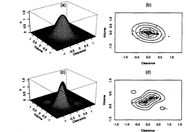
Fig.!. Estimated inter-individual random effects density and corresponding empirical Bayes

esti-mates, Case 2, no covariates. Panel (a) is the perspective plot of the estimated joint normal(K = 0) inter-individual random effects density and (b) is the contour plot at quantiles 10%, 25%, 50%, 75%, 90%, and 95% together with the empirical Bayes estimates of the random effects (dots). Panel (c) is the perspective plot of the estimated joint SNP(K

=

2) inter-individual random effects density and (d) is the contour plot at quantiles 10%, 25%, 50%, 75%, 90%, and 95% together with the empirical Bayes estimates of the random effects (dots).

We begin the Case 2 analysis by fitting the SNP models K=O,2,3 usmg a log-linear inter-individual regression function

[27]

without covariates:

C1

=

exp(,l

+

Zl)

v

=

exp(,2

+

Z2)

ka = exp(,3)'

With these data it is essential to enforce positivity of the pharmacokinetic parameters during nonlinear optimization. In other data sets we have found that this complication does not arise and enforcement of positivity during computations is not as important. One would, however, be unlikely to tolerate a specification whose converged estimates were negative for any admissible setting of the covariates or inter-individual random effects, which is a tedious condition to verify. The log-linear specification enforces positivity during computations and eliminates the need to check for global positivity.

factors to induce multi-modal estimates is seen in the J(

=

2 plots as is the separation of

empirical Bayes estimates of the inter-individual random effects.

The separation is due to omitted covariates in the inter-individual regression. Thus, for each pharmacokinetic parameter, a univariate regression of each individual's estimated random effect on his demographic attribute suggests the importance of that attribute as a covariate in the inter-individual regression function. A regression against measured con-centration reveals the importance of all omitted covariates taken as a group. It is easier to interpret a univariate regression when it is overlaid upon a scatter plot of the underlying data. Omitted curvilinearity that attenuates slope, influential outliers, and other characteristics can be immediately assessed by eye. When the data are categorical rather than measured along a continuum, boxplots take the place of scatter plots. Examples and a description of boxplots are in Figure 2.

The shallow slope of the regression of the empirical Bayes estimate of the V random effect on measured concentration in the lower panel of Figure 2 suggests that there are no omitted covariates in the V equation. The steep slope for the C1effect in the upper panel does suggest omitted covariates in the C1 equation.

To determine these omitted covariates, we inspect the remaining plots in the upper panel of Figure 2. Slopes for the regressions for categorical variables are not comparable to the slopes for continuous variables; comparisons must be made within variable types. On this basis, creatinine clearance is the most important categorical variable. Next in importance is race. But the race relationship is due entirely to Blacks, as seen from the graph, of which there are only ten in the sample; thus, we do not include race as a covariate. No other categorical variables seem as important. aI-acid glycoprotein concentration is the most important continuous variable. It is hard to judge between age, height, and weight as next in importance. These are correlated variables in these data, anyone of them could be expected to proxy for the other two; we selected weight. No other continuous variables seem as important.

The graphical analysis implies the inter-individual regression model

Clearance Random Effect

'"

..

'"

I .

'"

I

..

.

...

-:.:.;. .

..

: : •• I : •

0.

r---.:- :.:..-:::

:a::.

I 0. • I : I :I '1i

..

_....:a;.:

_··:oil'.

-

..

l - _{. ! .. :}i_i :.

-:.- =-= . .

.

..

: : I . I ·

~ <?

","a. glucon8te Doe-oelorm

tin ~n black ARe

oW eo 80 70 80 90 60 66 70 75 Age HeIght

'"

'"

..

..

~

..

0.

'"

'?

--

'"'?

-

-• otherwtee yea no pntIIiously

Smoking status Ethanol abuBe

60 80 100 120 Weight

mUd mode... severe ConO_IIYeheart failure

<50 >50

Creatinine c. .,.nce

~

.

....

.

.,_-. ~

0. -;...:"1....: 0.

..

..

...

_'"

'? '?

0 1 2 3 4 5

Albumin concan_lion

50 100 150 200 250 300

Glycoprotein concentration Quinidine concentration2 4 6 8

'.

60 80 100 120 Weight

..

d

:,"':=.:~.":'....:

t---~"';"riir--o--:"-i~~...

_.'.

~:",,:~:""::r+,:"'--j_~...

.",

:-

...

. . .

Volume Random Effect

..

..

d d

..

• • "'-..:..J.:I ...:... _"

..

.e: .' ': Iiii

i::··

d

...

:"'

...

~.

...

d . l I l l i j l

..

_:

...

_~

'? .' :

oW 50 60 70 80 90 60 66 70 75 Age Height

=

au ate g cona18

Dougeform

in caucalian bladl

Race

smoker otherwise

Smolcingat...

yes no preYioualy

Ethanol abuse

mUd moderate BeVent

COng_livehurt fllilure

<60 >50

Creatinine cI...noe

~

_'"

..

j

.

...;..It-:.:-0. 0.

..

I ""''';'J(''''-

..

-:-...

.

... '?

.

'?

o 1 2 3 4 5

Albumin c:oncentration

50 100 150 200 250 300

Gl')I'coprotein concentnltion OuIridine QOfIcentradon2 4 6 8

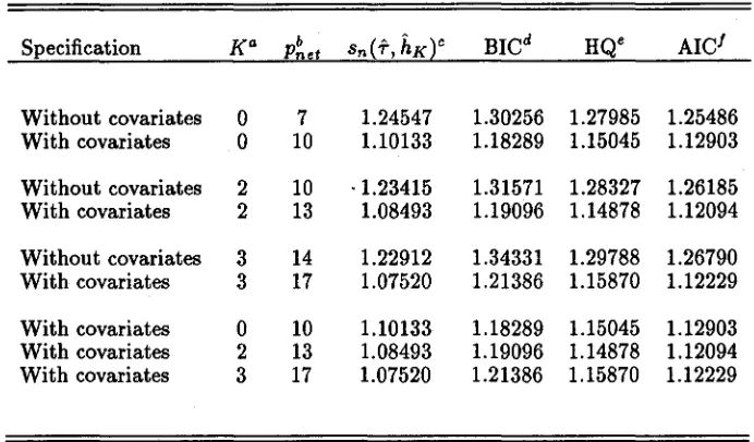
Table I. Optimization Results, Case 2, Covariates: Weight, at-acid Glycoprotein Concentration, Creatinine Clearance

Specification Ka P~et sn(f,hKt BICd HQe AIel Without covariates 0 7 1.24547 1.30256 1.27985 1.25486 With covariates 0 10 1.10133 1.18289 1.15045 1.12903

Without covariates 2 10 ·1.23415 1.31571 1.28327 1.26185 With covariates 2 13 1.08493 1.19096 1.14878 1.12094

Without covariates 3 14 1.22912 1.34331 1.29788 1.26790 With covariates 3 17 1.07520 1.21386 1.15870 1.12229

With covariates 0 10 1.10133 1.18289 1.15045 1.12903 With covariates 2 13 1.08493 1.19096 1.14878 1.12094 With covariates 3 17 1.07520 1.21386 1.15870 1.12229

aK is the degree of the polynomial part ofhK.

b_pnet is the effective number of parameters.

Csn(f,hK) is the negative of the optimized log-likelihood divided by the total

num-ber, N = 361, of measured concentrations. dBIC is the Schwarz model selection criterion. eHQ is the Hannan-Quinn model selection criterion.

IAIC is the Akaike model selection criterion.

For this model, we repeated the computations and graphics, reporting them as Table I, Figure 3, and Figure 4.

In Table I, the inclusion of weight, creatinine clearance, and aI-acid glycoprotein concen-tration in theC1equation is strongly supported by all criteria in all specifications,K

=

0,2,3. For the models with covariates, the conservative BIC criterion selects the normal (K = 0), and HQ and AIC criteria select the K = 2 specification.

As seen from Figure 3, the covariates have removed the multimodalityin the SNP (K = 2) estimate which suggests that there may no longer be omitted covariates.

The lower panel of Figure 4 indicates that there are no omitted covariates in the V

... N :::.: ••

:! .

...

... ·· ..(a) ... .... ". ". ~ on ~ 0 :> ~ ~ \ III -1.0 -0.5 (b) 0.0 Clearance 0.5 1.0

N ::: •••••..•.••..•...•..•···(c>'I"··· .

.... : ~

_....

; III_o o .,::; -1.0 (d)

~

..

-0.5 0.0 0.5

Clearance

1.0

Fig. 3. Estimated inter-individual random effects density and corresponding empirical Bayes esti-mates, Case 2, covariates: weight, aI-acid glycoprotein concentration, creatinine clearance. Panel (a) is the perspective plot of the estimated joint normal (K

=

0) inter-individual random effects density and (b) is the contour plot at quantiles 10%, 25%, 50%, 75%, 90%, and 95% together with the empirical Bayes estimates of the random effects (dots). Panel (c) is the perspective plot of the estimated joint SNP (K= 2) inter-individual random effects density and (d) is the contour plot at quantiles 10%, 25%, 50%, 75%, 90%, and 95% together with the empirical Bayes estimates of the random effects (dots).

as are those for all variables.

In the upper panel, the slope of the regression of the CI effect against quinidine concen-tration has been considerably attenuated from Figure 2. It is interesting to note that the plots for weight, aI-acid glycoprotein concentration, and creatinine clearance are flat. This attenuation and the shallow slopes of the regressions against the other variables suggests that there are no omitted covariates.

To confirm this impression, we computed the BIC, HQ, and AIC criteria for inclusion of each of dosage form, age, height, race, ethanol abuse, and congestive heart failure as an incremental variable in the equation

Cl

=

exp[,I

+

'4(weight)

+

,s(glyco.)

+

/6(creat.)

+

ZI]

Clearance Random Effect

.. ~

'"

•• ..:••••••1 ••:... 0 • • • • : ;. . . .

• • I ' . i . . ' I.~..-:...;..;.-r+i+ii-t'':'''''--''~ I-..-.:.i'·i':·if..:'::·~~~·~·1r::~·7·..-j

{--="'--II!!II---l ~ j-...:...~...t:I_~.~",••~.-:-""",.::,..---l ~ I " ' ! ' ~r •I ....,• •' . " . •

.

_.

_;:-~

.

_{: .}.. :" .: . I, Ie:!.' '.:- :--.

~ ~

"l_co

--

--..

co

..

~

~

<1

... lta. ucon"

Dougeform

~5080708090 Age

60 6S 70 76

Height 60 Weight80 100 120

f - -• •--.D---I~L.-!..--=I--l..-l~r;....--!'!!--l=--l

"l_co

--..

co

~

--~ r'iii---~--~!!!!!II-J

latin caue-llian black Race

smoker otherwiee

Smoking staws

yes no preYiously

Ethanolab.8e

mild moderate aewtf'8

COngeetive heart f.llure

.'

..

~

...

_...

':... '

..

--: .,

~... .: .

~J

--.11---1==--1

~M

1!F===--...

-I-.~:.o~...io:.:-i-•.,...~ ~ l--'~.~•.c~,.~.";~i.:-.- ...---=-t

r- ':: •

.

.,.;."';0 •

.

• :~.ih..•:.--o--. •

~

<50 >50

Creatinine clearance

o 1 2 3 4 6

Albumin conoentration

60 100 160 200 260 300

Glycoprotein concentration

2 4 6 6

Quinidine concentllltion

Volume Random Effect

..

..

..

"l

0

--

0 0 co

~ """":'= ....,.:c ...

.

..• : •• I : .

.. ·

:

.

"

co co _~ co _". ..::...

.

...

0 0

.

~;;

...• :"..-=-"'.

I _{: I .}

""

0

:t

• ''''''. ree.

.

~

--

·

.

_~

"l

--

"l "l "l ~

q q q q

.mate gJJconate _{~ 60 80 70 80 90 80 6S 70 76 «l 80 80 100 120}

Dougeform Age Height Weight

'"

~ '" "l

co co - co

-

₌₌

l!!!!!= Jii!Ii =

co co co co

0

~ 0 0 0 _.::::

== _- ...:.-

_--

_-

-

_-

-~

-

..

<1

--

..

<1 ~

IBtln _ a n black smoker otherwise yes no pralliously mild modBnlte _"vent

Raoe Smoking lItatus Ethilinol abuse Congestive heart failure

'"

'"

'"

'.

'"

.

co co co co

.

...i-

.

' ' ' : ' . L ·.,.·• • 'z,~"':'"'•

.

..

~

..

..

..

..

..

co co _...-...7"'" co

.

....;.,

... co .,

~

--'"

~ ~.

~

_'"

q q

<60 >60 _{0 1 2 3 4 6 60 100 160 200 260 300 2 4 6 6} C~tininea_ranee Abumln concentration Glycaproteln concentration Quinidine concentration

specification but does not support inclusion of any covariates when K = 2.

Because[23] reported lowered clearance for serious liver failure or serious congestive heart failure, we converted the tri-variate ethanol abuse and congestive heart failure variables to bi-variate categories by pooling non- or social drinkers with the ex-abusers and no or mild congestive heart failure patients with those experiencing moderate heart failure and repeated the above analysis, including both of the new variables simultaneously. For the K = 0 specification both the HQ and AIC criteria support inclusion of these covariates. ForK = 2,

only the AIC supports inclusion.

The graphical analysis in Cases 1 and 3 leads to the same log-linear specification of the inter-individual regression equation for 01 and V as for Case 2. In Case 3, the equation ka is log-linear without covariates, ka = exp(13

+

Z3).

Results

We found that no measured individual attributes affect the absorption rate ka or the

apparent volume of distributionV. We found that clearance01is positively related to weight, decreased in patients with impaired renal function (creatinine clearance

<

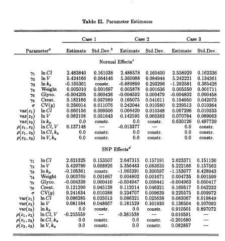
50), and decreased by increased levels of aI-acid glycoprotein concentration. We found weak statistical evidence that clearapce may be reduced in patients with severe congestive heart failure or ethanol abuse. These results agree with previous results as summarized above.

Parameter estimates for Cases 1, 2, and 3and specificationsK

=

0 and K

=

2are shown in Table II for the inter-individual regression

01

=

exp[,1

+

,4(weight)

+

15 (glyco.)

+

16(creat.)] exp(zl)

V = exp(,2)exp(z2)

ka

=

exp(,3)exp(z3)

where Z3 is interpreted as having zero variance in Cases 1 and 2. Estimates of the fixed

Table II. Parameter Estimates

Case 1 Case2 Case3

Parametera Estimate Std.Dev. b Estimate Std.Dev. Estimate Std.Dev.

Normal EffectsC

11 InCI 2.483840 0.161038 2.488578 0.160400 2.558929 0.162336 12 In V 5.424166 0.064146 5.360088 0.084944 5.242221 0.134361

IS Inka -0.105361 constr. -0.889899 0.293296 -1.292581 0.365426 14 Weight 0.005010 0.001697 0.005878 0.001636 0.005550 0.001711

IS Glyco. -0.004205 0.000426 -0.004592 0.000479 -0.004802 0.000458 16 Creat. 0.182166 0.037989 0.165075 0.041611 0.154950 0.042073

u CV(y) 0.250014 0.011076 0.242044 0.010580 0.239513 0.010364

var(zI) InCI 0.060156 0.009506 0.066420 0.010348 0.067296 0.010333

var(z2) In V 0.082108 0.051643 0.142595 0.066383 0.070784 0.089063

var(zs~ In ka 0.0 constr. 0.0 constr. 0.630126 0.497739

P(Z1,Z2 InCI, V 0.137148 -0.013377 0.0 constr.

P(Z1,ZS) InCI, ka 0.0 constr. 0.0 constr. 0.0 constr.

P(Z2,zs) In V, ka 0.0 constr. 0.0 constr. 0.0 constr.

SNP Effect~d

11 InCI 2.621325 0.153507 2.647315 0.157191 2.623371 0.151130 12 In V 5.429789 0.068826 5.356483 0.083635 5.222166 0.157562

IS Inka -0.105361 constr. -1.065291 0.300597 -1.153077 0.428943 14 Weight 0.003769 0.001667 0.004802 0.001671 0.004735 0.001599 15 Glyco. -0.004338 0.000410 -0.004947 0.000441 -0.004963 0.000417 ,6 Creat. 0.121290 0.045138 0.112014 0.046321 0.169517 0.042232

u CV(y) 0.241634 0.010388 0.234707 0.009639 0.225575 0.009972

var(z1~ InCI 0.086285 0.025013 0.086321 0.025638 0.083067 0.019849

var(z2 InV 0.081184 0.048667 0.181529 0.101930 0.136504 0.107092

var(zs) Inka 0.0 constr. 0.0 constr. 0.910501 0.897072 P(Z1,Z2) InCI, V -0.215559 -0.381538 0.010591

P(Z1,ZS) InCI, ka 0.0 constr. 0.0 constr. -0.201680

P(Z2,ZS) In V, ka 0.0 constr. 0.0 constr. 0.082857

aModel: The intra-individual pharmacokinetic model, represented as y = f(x,{3)

+

e, is a one-compartment open model with first-order absorption where {3= (C/, V, ka ) are the

pharmacoki-netic parameters, CIis clearance in L/hr, V is the apparent volume of distribution in L, andka is the absorption rate constant in hr- 1. Quinidine concentration, y, is in mg/L, and the experi-mental variablesx = (dose,time) are in mg of quinidine base and hr respectively. The errorseare normal with mean zero and standard deviation uf(x,{3). The inter-individual regression model for the pharmacokinetic parameters is InCI = 11

+

14(weight)

+

Is(glyco.)

+

16(creat.)

+

Zl, InV = 12

+

Z2, _{and Inka} = IS

+

Zs where the z's are the random effects. Weight is in kg, a1-acid glycoprotein concentration is in mg/dl, and creatinine clearance is in mljmin. Var(·) denotes the variance of a random effect and p(.,.) a correlation. Cases differ with respect to which parameters are constrained.

bconstr. means that the estimate is constrained to have the value shown.

Table III. Population Characteristics of the Random Effects

Case 1 Case 2 Case3

Characteristica Estimate Estimate Estimate

Normal Effectsb

CV(exp zt) GI 0.248875 0.263182 0.269232

CV~exp Z2~ V 0.299589 0.401253 0.277401

CVexp z3 ka 0.0 0.0 0.931264

£~exPzl~ GI 1.026680 1.030480 1.039373

£ exp Z2 V 1.039255 1.071143 1.037394

£(expZ3) ka 1.0 1.0 1.361435

var(exp zt) GI 0.065288 0.073551 0.078306

var~exp Z2~ V 0.096939 0.184727 0.082814

var expZ3 ka 0.0 0.0 1.607458

P~exp Zl, expZ2~ GI, V 0.111926 -0.036051 0.0

Pexp Zl , expZ3 GI,ka 0.0 0.0 0.0

p(expZ2,expZ3) V,ka 0;0 0.0 0.0

SNP EffectsC

CV~exp Zl~ GI 0.321833 0.314340 0.327505

CV expZ2 V 0.288746 0.537890 0.387419

CV(exp z3) ka 0.0 0.0 1.684499

rpZ1j

CI 1.042353 1.040531 1.050885

£ expZ2 V 1.035648 1.105573 1.075237

£ exp Z3 ka 1.0 1.0 1.647813

var~exp Zl~ GI 0.112536 0.106982 0.118453

var expZ2 V 0.089424 0.353640 0.173528

var(expZ3) ka 0.0 0.0 7.704733

p(exp Zl, expZ2) GI, V -0.193330 -0.319158 0.026915 P~exp Zl, expZ3~ GI, ka 0.0 0.0 -0.079568

pexpZ2,expZ3 V,ka 0.0 0.0 0.026544

aModel: The inter-individual regression model for the pharmacokinetic parameters is GI = exp['y! + 'Y4(weight) + 'Y5(glyco.) + 'Y6(creat.) + Zl],

V

=

exp(-Y2+z2), andka

=

exp('Y3+Z3) whereGIis clearance in L/hr,V is the apparent volume of distribution in L, ka is the absorption rate constant

in hr- l , and the z's are the random effects. Weight is in kg, ol-acid

gly-coprotein concentration is in mg/dl, and creatinine clearance is in ml/min.

GV(.) denotes the coefficient of variation of a random effect, £ (.) denotes the mean, var(·) the variance, and p(.,.) a correlation. Cases differ with respect to which parameter estimates are constrained, see Table II. The moments are computed by Monte Carlo integration using2000repetitions. bNormal Effects: maximum likelihood estimates with normal (/{

=

0) ran-dom effects density.

The population characteristics of [exp(zl), exp(z2), exp(z2)] are required in order to as-sess the population characteristics of the pharmacokinetic parameters as is seen from the inter-individual regression equations for

f3

= (Gl, V, ka ) above. Since it is easy to

sim-ulate from the SNP density

[12],

as noted above, an estimate of a population charac-teristic such as a mean £exp(zl)

=

Jexp(zdhO(z) dz can be computed by Monte Carlo integration by drawing a sample

{zdI=1

from the estimated SNP density

h

K and

av-eraging

t

exp(zl) ..:. (1/1)2:[=1 exp(zli)' Similarly, a percentile would be computed as the corresponding percentile of {exp(zli)}!=I' These computations can be made as accu-rate as desired by taking the number of Monte Carlo repetitions I large enough. Using this procedure, the coefficients of variation, the means, the variances, and correlations of [exp(zl), exp(z2), exp(z2)] were computed and are shown in Table III for Cases 1, 2, and 3 and specifications K

=

0 and 2.

The most notable feature of Table III is the high coefficient of variation of exp(z3), which corresponds to absorption rate ka , and its interaction with the coefficient of variation of

exp(z2)' which corresponds to volume V. Treating ka as a fixed parameter to be estimated,

Case 2, increases the coefficient of variation of volume over both the case whenka is fixed and

specified, Case 1, and when treated as a random effect, Case 3. This is apparently due to an insufficient number of samples collected during the absorption phase. It is also interesting to note the stability of population characteristics of exp(zl), which corresponds to quinidine clearanceGl, across Cases 1, 2, and 3.

Because the inter-individual regression model is multiplicative, estimates of the popula-tion characteristics of the pharmacokinetic parameters are obtained by rescaling the random effect estimates. For instance, at a given setting of weight, aI-acid glycoprotein concentra-tion, and creatinine clearance

tel

=

exp[1I +14(weight)

+

1s(glyco.)

+

16(creat.)]£ exp(zd

SiJ(Gl)

=

exp[1I

+

14(weight)

+

1s(glyco.)

+

16(creat.)]v/@(expzd

where

t

exp(zl) and

Vaf(

expZl) are the entries from Table III. TableIVdisplays estimates of population characteristics of the pharmacokinetic parameters

f3

=

(Gl, V, ka ) at some

Table IV. Population Characteristics of the Pharmacokinetic Parameters

Case 1 Case 2 Case 3

Characteristica Estimate Estimate Estimate

Normal Effectsb

£Gl: low weight, low glyco., creat.<50 12.374220 12.788633 13.378630 low weight, low glyco., creat.>50 14.846755 15.083957 15.620883 low weight, median glyco., creat.<50 10.262462 10.425062 10.804575 low weight, median glyco., creat.>50 12.313039 12.296169 12.615417 low weight, high glyco., creat.<50 7.957304 7.896319 8.080459 low weight, high glyco., creat.>50 9.547280 9.313563 9.434740 median weight, low glyco., creat.<50 13.678364 14.384003 14.949213 median weight, low glyco., creat.>50 16.411483 16.965667 17.454695 median weight, median glyco., creat.<50 11.344043 11.725579 12.072977 median weight, median glyco., creat.>50 13.610735 13.830105 14.096403 median weight, high glyco., creat.<50 8.795940 8.881378 9.029063 median weight,hi~h glyco., creat.>50 10.553487 10.475422 10.542331 high weight, low g yeo., creat.<50 15.426014 16.563289 17.079154 high weight, low~lyco., creat.>50 18.508337 19.536094 19.941613 high weight, median glyco., creat.<50 12.793443 13.502093 13.793116 high weight, median glyco., creat.>50 15.349744 15.925470 16.104837 high weight, high glyco., creat.<50 9.919776 10.226974 10.315511 high weight, high glyco., creat.>50 11.901879 12.062527 12.044386

£V 235.725999 227.878890 196.160421

£ka 0.9 0.410697 0.373797

SNP EffectsC

£Gl: low weight, low glyco., creat.<50 13.274630 13.860196 13.597986 low weight, low glyco., creat.>50 14.986423 15.503025 16.109975 low weight, median glyco., creat.<50 10.944244 11.121494 10.903329 low weight, median glyco., creat.>50 12.355529 12.439709 12.917528 low weight, high glyco., creat.<50 8.417936 8.244829 8.075273 low weight, high glyco., creat.>50 9.503448 9.222076 9.567038 median weight, low glyco., creat.<50 14.313951 15.257347 14.948660 median weight, low glyco., creat.>50 16.159767 17.065778 17.710163 median weight, median glyco., creat.<50 11.801111 12.242575 11.986346 median weight, median glyco., creat.>50 13.322891 13.693670 14.200613 median weight, high glyco., creat.<50 9.077008 9.075933 8.877382 median weight, high glyco., creat.>50 10.247509 10.151690 10.517323 high weight, low glyco., creat.<50 15.669101 17.121058 16.747712 high weight, low~lyco., creat.>50 17.689667 19.150392 19.841559 high weight, median glyco., creat.<50 12.918361 13.738027 13.428887 high weight, median glyco., creat.>50 14.584213 15.366375 15.909639 high weight, high glyco., creat.<50 9.936359 10.184573 9.945763 high weight, high glyco., creat.>50 11.217675 11.391736 11.783069

£V 236.232459 234.357272 199.279249

£ka 0.9 0.344628 0.520155

aWeight: low, 10th percentile, 59.0 kg; median, 79.0 kg; high, 90th percentile, 103.0 kg. al-acid

glycoprotein concentration: low, 10th percentile, 69.0 mg/dl; median, 113.5 mg/dl; high, 90th percentile, 174.0 mg/dl. Creatinine clearance: creat. < 50 ml/min; creat. > 50 ml/min. Coefficients of variation and correlations for Gl, V, and ka are as for exp(zI), exp(za), and exp(za), respectively,

clearance.

DISCUSSION

We propose the SNP method, taken from the econometrics literature, for the analysis of population pharmacokinetic data that can be described by a nonlinear mixed effects model.

Itproduces smooth nonparametric estimates of the entire random effects density and simul-taneous estimates of fixed effects by maximum likelihood. The benefits of estimating the entire distribution nonparametrically rather than a few leading moments have been discussed in [7]. We also introduce a new graphical model building strategy that exploits an inherent tendency of a nonparametric method to produce disparate empirical Bayes estimates when covariates have been omitted from the model. We illustrate by an analysis of the population pharmacokinetics of quinidine.

Because the SNP method is based on the· principle of maximum likelihood and because the SNP density has a convenient representation, subsequent computations essential to a complete statistical analysis are straightforward: estimation of the precision of the estimates of fixed effects, statistical tests of the significance of covariates, tests for normality of the random effects density, empirical Bayes estimation of individual random effects, and esti-mation of population characteristics of pharmacokinetic parameters including those that are affected nonlinearly by the random effects. More elaborate, computationally intensive sta-tistical analyses are also possible such as setting sup-norm confidence bands on a marginal density of a random effect or pharmacokinetic parameter [10] or placing a global restriction on the density such as unimodality [9].

The SNP density estimate is inherently smooth; a subsequent smoothing computation is not required. Statistical inference is possible: one can test for normality and set confidence intervals on parameters.

If the true random effects distribution violates the smoothness assumption, however, the NPML estimator will be consistent and the SNP estimator will not. Empirical Bayes estimation of the random effects is convenient with both the SNP and NPML methods, and thus both allow use of the graphical model building strategy that we describe.

Mallet et ai. [7] compare the features of nonparametric methods to other procedures for

the analysis of the nonlinear mixed effects model: the popular first-order (FO) approximation with extended least squares (ELS) estimation [1, 28, 3], which provides estimates of fixed effects, allows empirical Bayes estimation based on normality, and is implemented in the powerful NONMEM package [29, 30]; and two-stage (TS) methods [31, 2]. Nonparametric methods are indicated when a knowledge of the entire distribution is required, not just first and second moments, and when there may be reason to doubt a parametric assumption, such as normality, for the purpose of computing empirical Bayes estimates, for example. Nonpara-metric estimation of the entire distribution may be based on the use of two-stage methods; these methods, however, require a sufficient number of observations on each individual to al-low accurate estimation of individual pharmacokinetic parameters. Thus, two-stage methods are usually not applicable to clinical data, which are typically sparse.

In addition, as we have illustrated here, nonparametric methods are inherently well suited to model building. Even when there is no other reason to use nonparametric methods, their unique ability to fragment empirical Bayes estimates, thereby exaggerating their relation to influential individual attributes, can be of value in allowing graphical screening of a large number of attributes for their potential as covariates.

References

[1] S. L. Beal, and1.B. Sheiner. Estimating population kinetics. GRG Grit. Rev. in Biomed.

Eng. 8:195-222 (1982).

estimation of population pharmacokinetic parameters: comparison with the nonlinear mixed effect model. Drug Metab. Rev. 15:265-292 (1984).

[3] S. 1. Beal and L. B. Sheiner. Methodology of population pharmacokinetics. In E. R. Garrett & J. L. Hirtz (eds.), Drug Fate and Metabolism-Methods and Techniques, Vol 5. Marcel Dekker, New York, 1985, pp. 135-83.

[4] L. B. Sheiner and T. M. Ludden. Population pharmacokinetics/dynamics. Annu. Rev.

Pharmacol. Toxicol. 32:185-209 (1992).

[5] S. Vozeh, R. Hillman, M. Wandell, T. M. Ludden, and L. B. Sheiner. Computer-assisted drug assay interpretation based on Bayesian estimation of individual pharmacokinetics: application to lidocaine. Ther. Drug. Monit. 7:66-73 (1985).

[6] A. Mallet. A maximum likelihood estimation method for random coefficient regression models. Biometrika 73:645-656 (1986).

[7] A. Mallet, F. Mentre, J-L Steimer, and F.Lokiec. Nonparametric maximum likelihood estimation for population pharmacokinetics, with application to cyclosporine. J. Phar-macokin. Biopharm. 16:311-327 (1988).

[8] A. R. Gallant and D. W. Nychka. Seminonparametric maximum likelihood estimation.

Econometrica, 55:363~390 (1987).

[9] A. R. Gallant and G. E. Tauchen. Seminonparametric estimation of conditionally con-strained heterogeneous processes: asset pricing applications. Econometrica 57:1091-1120 (1989).

[10] A. R. Gallant, P. E. Rossi, and G. E.Tauchen. Stock prices and volume. Rev. Finane.

Stud. 5:in press (1992).

[11] A. D. Brunner. Conditional asymmetries in real GNP: a seminonparametric approach.

• •

[12] M. Davidian and A. R. Gallant. The nonlinear mixed effects model with a smooth random effects density. Institute of Statistics Mimeo Series No. 2206. North Carolina State University, Raleigh, 1992.

[13] 1. Elbadawi, A. R. Gallant, and G. Souza. An elasticity can be estimated consistently without a priori knowledge of functional form. Econometrica 51:1731-1752 (1983). [14] A. R. Gallant. Identification et convergence en regression semi-nonparametrique. Annals

de l'INSEE59/60:239-267 (1985).

[15] S. L. Beal and L. B. Sheiner. Heteroscedastic nonlinear regresSIOn. Technometrics

30:327-338 (1988).

[16] N. L. Johnson and S Kotz. Gontinuous Univariate Distributions. Wiley, New York, 1970. [17] B. J. Eastwood. Asymptotic normality and consistency of semi-nonparametric regression estimators using an upward F test truncation rule. J. Econometrics48:151-182 (1991). [18] B. M. Potscher. Model selection under nonstationarity: autoregressive models and

stochastic linear models. Ann. Statist. 17:347-370 (1989).

[19] E. J. Hannan. Rational transfer function approximation. Statist. Sci. 2:1029-1054

(1987) .

[20] A. R. Gallant. Nonlinear Statistical Models. Wiley, New York, 1987.

[21] B. W. Silverman. Density Estimation for Statistics and Data Analysis. Chapman and Hall, London, 1986.

[22] H. R.Ochs, D. J. Greenblatt, and E. Woo. Clinical pharmacokinetics of quinidine. Glin.

Pharmacokin. 5:150-168 (1980).

[23] K. Fattinger, S. Vozeh, H. R. Ha, M. Borner, and F. Follath. Population pharmacoki-netics of quinidine. Br. J. Glin Pharmac. 31:279-286 (1991).

•

•

[25] American Statistical Association. Proceedings of the Biopharmaceutical Section, Annual Meetings, Boston, 1992 American Statistical Association, Alexandria VA, 1992.

[26] C. N. Verme, T. M. Ludden, W. A. Clementi, and S. C. Harris. Pharmacokinetics of quinidine in male patients: A population analysis. Glin. Pharmacokin. 23:in press (1992).

[27] M. S. Driscoll, T. M. Ludden, D. T. Casto, and 1. C. Littlefield. Evaluation of theo-phylline pharmacokinetics in a pediatric population using mixed effects models. J.

Pharamacokin. Biopharm. 17:141-168 (1989).

[28] S. L. Beal. Population pharmacokinetic data and parameter estimation based on their first two statistical moments. Drug Metab. Rev. 15:173-193 (1984).

[29] S. 1. Beal and L. B. Sheiner. The NONMEM system. Am. Statist. 34:118-119 (1980). [30] A. J. Boeckmann, L. B. Sheiner, and S. 1. Beal. NONMEM User's Guide, Part V,

Introductory Guide. University of California, San Francisco, 1990.

[31] L. B. Sheiner and S. 1.Beal. Evaluation of methods for estimating population pharma-cokinetic parameters. III. Monoexponential model: Routine pharmacokinetic data. J.