A High Accuracy Variant of The Iterative Alternating Decomposition Explicit Method for Solving The Heat Equation

(1)

Copyright © 2006 Inderscience Enterprises Ltd.

A high accuracy variant of the iterative alternating

decomposition explicit method for solving the heat

equation

M.S. Sahimi*, N.A. Mansor, N.M. Nor and N.M. Nusi

Department of Engineering Sciences and Mathematics,

Universiti Tenaga Nasional, 43009 Kajang, Selangor, Malaysia

E-mail: [email protected]

*

Corresponding author

N. Alias

Department of Mathematics,

Universiti Teknologi Malaysia,

81310 UTM Skudai, Johor, Malaysia

E-mail: [email protected]

Abstract:

We consider three level difference replacements of parabolic equations focusing on the

heat equation in two space dimensions. Through a judicious splitting of the approximation,

the scheme qualifies as an alternating direction implicit (ADI) method. Using the well known fact

of the parabolic-elliptic correspondence, we shall derive a two stage iterative procedure

employing a fractional splitting strategy applied alternately at each intermediate time step to the

one dimensional heat equation. As the basis of derivation is the unconditionally stable (4,2)

accurate ADI scheme, this method is convergent, computationally stable and highly accurate.

Keywords:

alternating direction implicit (ADI) method; iterative alternating decomposition

explicit (IADE) method; fractional splitting.

Reference

to this paper should be made as follows: Sahimi, M.S., Mansor, N.A., Nor, N.M.,

Nusi, N.M. and Alias, N. (2006) ‘A high accuracy variant of the iterative alternating

decomposition explicit method for solving the heat equation’, Int. J. Simulation and Process

Modelling, Vol. 2, Nos. 1/2, pp.45–49.

Biographical notes:

Mohd Salleh Sahimi obtained his BS from the Bandung Institute of

Technology, Indonesia (1975), MA from the University of Lancaster, UK (1976) and PhD from

the Loughborough University of Technology, UK (1986). He served in various academic

executive capacities in the Universiti Kebangsaan Malaysia including as Deputy Dean of the

Faculty of Mathematical and Computer Sciences (1994) and Deputy Dean of the Faculty of

Information Science and Technology (1997). He was awarded a Commonwealth Fellowship to

conduct research in the UK (1993). Presently, he is a Professor in Numerical and Scientific

Computing at the Department of Engineering Sciences and Mathematics, Universiti Tenaga

Nasional.

Noreliza Abu Mansor obtained her BSc in Physics (1982) and MSc in Mathematics (1985), both

from Ohio University, USA. She received her Diploma in Education (1988) from Universiti

Kebangsaan Malaysia. She started her career as a Teacher (1988) before joining as a Lecturer at

Kolej Yayasan Pelajaran Mara (1994). She is currently a Mathematics Lecturer in the Department

of Engineering Sciences and Mathematics, Universiti Tenaga Nasional.

Norhalena Mohd Nor obtained her BSc with honours in 1985 from the University of Tasmania,

Australia and MSc in Pure Mathematics from the University of Leeds in 1987. She started her

career as an Assistant Lecturer at the Universiti Teknologi Malaysia, Kuala Lumpur. Currently

she is a Senior Lecturer in the Department of Engineering Sciences and Mathematics at

Universiti Tenaga Nasional.

Noraini Md. Nusi obtained her B.App.Sc Degree from Universiti Sains Malaysia in 1997 and

MSc from Universiti Kebangsaan Malaysia in 2002. She is currently a Mathematics Lecturer in

the Department of Engineering Sciences and Mathematics, Universiti Tenaga Nasional.

(2)

computing in numerical methods for application in the manufacturing industry. She has also

published and presented about 50 papers related to variants of the iterative alternating

decomposition explicit and alternating group explicit class of methods. She has received various

awards including medals for invention and innovation in national and international expositions.

1 Introduction

Consider the heat equation,

2 2

U

t

x

∂

₌

∂

(1)

subject to given initial and Dirichlet boundary conditions

over a rectangular domain with a uniformly spaced network

whose mesh points are xi = i

∆

x,

tj = j

∆

t. Its corresponding

equation in two space is given by,

2 2

.

U

t

x

y

∂

₌

∂

₊

∂

(2)

Following (Mitchell and Griffiths, 1980), a stable and (4,2)

accurate three level difference replacement of equation (2)

is given by,

2 2

. . 1

2 2 2 2

, ,

2 2

, , 1

2

2 2

, , , , 1

1

2

1

2

1

1 12 3

12 3

2

1

3

2

1

2

1 (

)

12 3

1

2 (2

)

12 3

x y i j k

x y x y i j k

x y i j k

x y i j k i j k

u

λ δ

δ

δ δ

λ δ

δ

λ δ δ

+ − −



₊



₋





₊



₋































=

_

+

_









+ +



_

+



_

+











+

_

−

_

−





(3)

where

δ

is the usual central difference operator and

λ

=

∆

t/(

∆

x)

2

₌

_∆

_t/(

_∆

_y)

2

_{, the mesh ratio for equidistance}

spacing. The difference scheme equation (3) can be split as

follows, to qualify as an alternating direction implicit (ADI)

scheme,

2

, , 1/ 2

2

, , . . 1

2 2 2 2

, ,

2 2

, , 1

1

2

1 12 3

1

2 (2

)

12 3

2

1

3

2

1

2

1 (

)

12 3

x i j k

y i j k i j k

x y x y i j k

x y i j k

u

λ δ

δ

δ δ

λ δ

δ

+ − −



₊



₋





_



_











= −



−



−









+



+











+ +



_

+



_

+







(4)

and

2

, , 1 , , 1/ 2

2

, , , , 1

1

2

1 12 3

1

2 (2

).

12 3

y i j k i j k

u

λ δ

+ + −



₊



₋



₌



_



_











+

_

−

_

−





(5)

As the temperature reaches steady state over time,

U

→

constant and (

∂

U/

∂

t)

→

0 and the parabolic equation

(5) reduces to the elliptic equation (Laplace’s equation),

2 2

0 U

U

x

y

∂

₊

∂

₌

∂

(6)

whose numerical solution can be solved iteratively using the

same ADI technique,

(

)

2 ,

2 2 2 2 2

2 2 ( )

,

1

2 _*

1 12 3

1

2

1 12 3

3

2

1

2

1 12 3

x i j

y x y x y

p x y i j

r

u

r

u

δ

δ δ

δ





+

−













 







= −

_{ }

−



+



+



















+ +



_

+



_

+



_





(7)

and

2 ( 1) 2 ( )

, , ,

1

2 _*

1

2

1 12 3

12 3

p p

y

u

i j

u

i j

r

y i j

u

δ

+

δ



₊



₋



₌

₊



₋





_



_





_



_





(8)

where r is the acceleration parameter.

2 The iterative alternating decomposition explicit

(IADE) method

Note from the composite formula equation (3) that the

iterative procedure converges if

ui

,j,k–1

= ui

,j,k = ui,j,k+1

= ui

,j

for k sufficiently large, leading to

2 2 2 2

,

1 ₀

6

x y x y

u

i j

δ

δ δ



₊



₌









which represents a nine point difference replacement of the

Laplace’s equation (6). Hence we are motivated by this well

known fact of the parabolic-elliptic correspondence (Varga,

1962; Wachspress, 1966; Yanenko, 1971) to develop a new

iterative scheme for the solution of equation (1) by

considering the following two step iterates corresponding to

equations (7) and (8),

( +1/2)

1 2 1 2 1 2

( )

1 2

ˆ

( +

)

(

(1 2

)

(

))

2

p

_r

I

G u

G

G + G

)G G

I

G + G

u

f

α

ω

= −

+

+ +

−

(9)

and

(

I

+

α

G

2

)

u

(p+1)

=

u

(p+1/2)

+

α

G

2

u

(p)

(10)

(3)

1

2

1

2 _ˆ

2 ,

,

12 3

r

12 3

r

3 r

α

=

−

ω

=

+

ω

=

with

r > 0 being the acceleration parameter of the iterative

process.

Noting that

u

(p+1)

=

u

(p)

as p

→

∞

, we have,

at the (p + 1/2) iterate,

(

I

+

α

G

2

)

u

(p+1/2)

= (

I

+ (

α

+ 2r)

G

1

)(

I

+ (2r

G

2

)

+

β

G

1

G

2

)

u

(p)

– 2r

f

(11)

and at the (p + 1) iterate,

(

I

+

α

G

2

)

u

(p+1)

=

u

(p+1/2)

+

α

G

2

u

(p)

(12)

where

β

= 2r(3

α

– 2r)/3, and

G

1

and

G

2

are lower and upper

bidiagonal matrices given by,

1 2

1

2

1 ( )

1

1 .

.

,

.

1

m m mxm

k

− −

























=

_

_

























G

(13)

1 2 3 2 1 ( )

.

m m mxm

e

h

e

h

e

h

e

h

e

−

























=

_

_

























G

(14)

Elimination of

u

(p+1/2)

_{from equations (11) and (12) leads to}

the single composite formula,

(

I

+

α

G

1

)(

I

+

α

G

2

)

u

(p+1)

= ((

I

+ (

α

+ 2r)

G

1

)(

I

+ 2r

G

2

) +

β

G

1

G

2

)

u

(p)

– 2r

f

+

α

(

I

+

α

G

1

) +

G

2

u

)

(p)

.

As p

→

∞

,

u

(p)

,

u

(p+1)

→

u

resulting in

1 2 1 2

1

6 =

+

A G

G

G G

(15)

and

Au

=

f

(16)

A

is a tridiagonal matrix which arises from the difference

method used to approximate the parabolic equation (1). For

example, if the familiar weighted approximation,

1, 1 , 1 1, 1

1, 1,

(1 2

)

(1

)

(1 2 (1

))

(1

)

i j i j i j

i j ij i j

u

λθ

λ

θ

λ

θ

λ

θ

− + + + + − +

−

+ +

−

=

−

+ −

−

+

−

is used with order of accuracy of (1,2), (2,2), (2,4) and (1,2)

when

θ

= 1, 1/2, (1/2 – 1/12

λ

) and 0 respectively, then its

totality can be displayed in matrix form equation (16) as,

1 1

2 2

3 3

1 1

( ) 1

.

m m m m mxm j

u

f

a b

u

f

c a b

u

f

c a b

u

f

c a b

u

f

c a

− − +









































































₌





















































































(17)

Using equations (11) and (12), we have,

u

(p+1/2)

_{= (}

_I

₊

_α

_G

1

)

–1

((

I

+ (

α

+ 2r)

G

1

)(

I

+ (2r

G

2

)

+

β

G

1

G

2

)

u

(p)

– 2r

f)

(18)

and

u

(p+1)

_{= (}

_I

₊

_α

_G

2

)

–1

(

u

(p+1/2)

+

α

+

G

2

u

(p)

)

(19)

giving us the following computational formulae at each of

the half-iterates,

at the (p + 1/2) iterate,

( 1/ 2) ( ) ( ) ( ) ( 1/ 2)

1 1

ˆ

1 1 1

(

* ) / ,

1, 2, ,

p p p p p

i i i i i i i i i

u

s u

v u

su

w u

r f

A

i

m

+ +

− − + − −

=

+

−

=

…

(20)

with

s

0

=v

0

= w

0

= 0 and

1 (1 8 )

0

12 r

A

= +

+

≠

at the (p + 1) iterate,

( 1) ( 1/ 2) ( ) ( )

1 1 1 1 2

( 1)

2 1

(

) /(1

)

p p p p

m i m i m i m i m i p

m i m i

u

d

u

du

d

+ + + − + − + − + − + − + + − + −

=

+

−

+

(21)

with di

≠

0 for i = 1, 2 ,

…

, m and

1

1 1 1 1

1

1 1

6 1 8

*

2 ,

,

7

12 *(3

*)

_,

_{2 ,}

_ˆ

_{* ,}

3 ˆ

_,

_ˆ

_{( *}

_),

_,

6(

1)

6 ˆ 1

,

7

6

6 _{1 ,}

_{2,3, ,}

7

6 ,

1, 2, ,

1 *

(

),

,

i i

i i i i

i i i

r

h

b

r

q

P

r

f

r P

g

f

q

s h r

f

q

d

h

a

c

A

e

k

e

k h

e

a

i

m

s

Pk

gk e

i

m

v

r e

P g hk

e

w

k

d

…

α

_α

α

+ − − − − − − =

+

= −

=

−

=

= −

=

= +

=

+ +

=

−

= +

=

+





=

_

−

_

=





=

+

=

= +

+ +

+

=

_α

e

_i

,

i

=

1, 2, , .

…

m

(4)

each iterate, the solution of an explicit equation. This is

continued until convergence is reached, that is, when the

convergence requirement ||

u

(p+1)

_–

_u

(p)

_||

∞

≤

ε

is met where

ε

is the convergence criterion.

3 Numerical

results

In this experiment we attempted to solve the following heat

conduction problem (Saulev, 1964),

2

0

1 U

U

x

t

x

∂

₌

∂

_{≤ ≤}

∂

(22)

subject to the initial condition

U

(

x

, 0) = 4

x

(1 –

x

) 0

≤

x

≤

1 and the boundary conditions

U

(0,

t

) =

U

(1,

t

) = 0

t

≥

0. The exact solution is given by

2 2

3 3

1,(2)

32

1 ( , )

k t

sin(

).

k

U x t

e

k x

k

π

_π

π

∞

−

=

∑

(23)

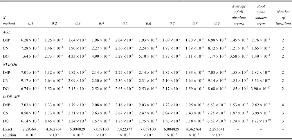
Tables 1–3 provide a comparison of the accuracy of the

methods under consideration in terms of the absolute errors

as well as the root mean square error at the appropriate grid

points for mesh ratios

λ

= 0.1,

λ

= 0.5 and

λ

= 1.0 at time

levels of

t

= 0.05,

t

= 0.25 and

t

= 0.5. The results in these

tables amply demonstrate that this new variant of the IADE

(NVIADE) method has comparable accuracy with the

highly accurate AGE method of the Peaceman-Rachford

(Tien and Chawla, 1989) variant as well as the IADE

scheme using the Mitchell-Fairweather variant (Sahimi

et al., 1993). This is even more apparent when the (2,4)

accurate Douglas finite difference approximation is used to

approximate the parabolic equation (1). As the basis of

derivation is the unconditionally stable (4,2) accurate ADI

scheme, the NVIADE method is convergent and

computationally stable and its accuracy compares well with

the (4,2) accurate IADE-MF and (2,2) accurate AGE.

Table 1

Absolute errors of numerical solutions

λ

= 0.1,

t

= 0.05,

∆

t

= 0.001,

∆

x

= 0.1,

eps

= 10

–4

X

method 0.1 0.2 0.3 0.4 0.5 0.6 0.7 0.8 0.9

Average of all absolute

errors

Root mean square

error

Number of iterations Age

IMP 1.47 × 10–3_2.63_×₁₀–3_3.34_×₁₀–3_3.67_×₁₀–3_3.76_×₁₀–3_3.67_×₁₀–3_3.35_×₁₀–3_2.63_×₁₀–3_1.47_×₁₀–3_2.89_×₁₀–3_9.07_×₁₀–6₂

CN 9.15 × 10–4_1.64_×₁₀–3_2.09_×₁₀–3_2.30_×₁₀–3_2.36_×₁₀–3_2.30_×₁₀–3_2.09_×₁₀–3_1.64_×₁₀–3_9.15_×₁₀–4_1.81_×₁₀–3_3.56_×₁₀–6₂

DG 1.67 × 10–6

5.49 × 10–6

1.15 × 10–5

1.72 × 10–5

1.97 × 10–5

1.73 × 10–5

1.15 × 10–5

5.52 × 10–6

1.60 × 10–6

1.01 × 10–5

1.46 × 10–10

2

NVIADE

IMP 1.49 × 10–3_2.64_×₁₀–3_3.35_×₁₀–3_3.67_×₁₀–3_3.75_×₁₀–3_3.67_×₁₀–3_3.35_×₁₀–3_2.64_×₁₀–3_1.47_×₁₀–3_2.89_×₁₀–3_9.08_×₁₀–6₂

CN 9.17 × 10–4_1.64_×₁₀–3_2.10_×₁₀–3_2.31_×₁₀–3_2.36_×₁₀–3_2.31_×₁₀–3_2.10_×₁₀–3_1.64_×₁₀–3_9.14_×₁₀–4_1.81_×₁₀–3_3.57_×₁₀–6₂

DG 2.47 × 10–6 _1.50_×₁₀–7 _1.33_×₁₀–6 _4.09_×₁₀–6 _4.32_×₁₀–7 _1.23_×₁₀–7 _3.30_×₁₀–7 _5.89_×₁₀–7 _4.12_×₁₀–6 _4.13_×₁₀–6 _1.22_×₁₀–11₂

IADE-MF

IMP 1.07 × 10–3_1.88_×₁₀–3_2.74_×₁₀–3_3.19_×₁₀–3_3.36_×₁₀–3_3.34_×₁₀–3_3.11_×₁₀–3_2.59_×₁₀–3_1.65_×₁₀–3_2.55_×₁₀–3_9.07_×₁₀–6₄

CN 7.94 × 10–4_1.43_×₁₀–3_1.86_×₁₀–3_2.07_×₁₀–3_2.14_×₁₀–3_2.11_×₁₀–3_1.95_×₁₀–3_1.55_×₁₀–4_8.71_×₁₀–4_1.64_×₁₀–3_3.53_×₁₀–7₃

DG 5.84 × 10–6 _8.46_×₁₀–6 _3.74_×₁₀–7 _8.94_×₁₀–6 _1.38_×₁₀–5 _1.35_×₁₀–5 _9.28_×₁₀–6 _4.48_×₁₀–6 _1.39_×₁₀–6 _7.34_×₁₀–6 _1.35_×₁₀–10₃

Exact solution

0.1950648 0.3707705 0.5098716 0.5989617 0.6296137 0.5989617 0.5098716 0.3707705 0.1950648 – – –

Table 2

Absolute errors of numerical solutions

λ

= 0.5,

t

= 0.25,

∆

t

= 0.005,

∆

x

= 0.1,

eps

= 10

–4

X

method 0.1 0.2 0.3 0.4 0.5 0.6 0.7 0.8 0.9

errors

Root mean square

error

Number of iterations Age

IMP 2.18 × 10–3_4.15_×₁₀–3_5.69_×₁₀–3_6.70_×₁₀–3_7.04_×₁₀–3_6.69_×₁₀–3_5.71_×₁₀–3_4.14_×₁₀–3_2.19_×₁₀–3_4.94_×₁₀–3_2.76_×₁₀–5₂

CN 5.32 × 10–4_1.02_×₁₀–3_1.39_×₁₀–3_1.64_×₁₀–3_1.72_×₁₀–3_1.64_×₁₀–3_1.40_×₁₀–3_1.01_×₁₀–3_5.43_×₁₀–4_1.21_×₁₀–3_1.65_×₁₀–6₂

DG 7.38 × 10–6 _2.05_×₁₀–5 _3.06_×₁₀–5 _3.77_×₁₀–5 _4.11_×₁₀–5 _4.53_×₁₀–5 _3.62_×₁₀–5 _2.76_×₁₀–5 _1.17_×₁₀–5 _3.23_×₁₀–5 _1.20_×₁₀–9₂

NVIADE

IMP 2.23 × 10–3_4.19_×₁₀–3_5.76_×₁₀–3_6.77_×₁₀–3_7.11_×₁₀–3_6.77_×₁₀–3_5.75_×₁₀–3_4.18_×₁₀–3_2.19_×₁₀–3_5.00_×₁₀–3_2.82_×₁₀–5₂

CN 5.47 × 10–4

1.03 × 10–3

1.41 × 10–3

1.65 × 10–3

1.74 × 10–3

1.65 × 10–3

1.40 × 10–3

1.02 × 10–3

5.32 × 10–4

1.22 × 10–3

1.68 × 10–6

2 DG 7.38 × 10–6 _2.05_×₁₀–6 _3.06_×₁₀–5 _3.77_×₁₀–5 _4.11_×₁₀–6 _4.04_×₁₀–5 _3.57_×₁₀–5 _2.74_×₁₀–5 _1.63_×₁₀–5 _2.85_×₁₀–5 _9.37_×₁₀–10₂

IADE-MF

IMP 2.20 × 10–3_4.19_×₁₀–3_5.76_×₁₀–3_6.76_×₁₀–3_7.10_×₁₀–3_6.75_×₁₀–3_5.74_×₁₀–3_4.17_×₁₀–3_2.19_×₁₀–3_4.98_×₁₀–3_2.81_×₁₀–5₃

CN 5.37 × 10–4_1.02_×₁₀–3_1.41_×₁₀–3_1.65_×₁₀–3_1.74_×₁₀–3_1.65_×₁₀–3_1.41_×₁₀–3_1.02_×₁₀–4_5.38_×₁₀–4_1.22_×₁₀–3_1.68_×₁₀–6₃

DG 8.14 × 10–6

2.53 × 10–5

3.40 × 10–5

3.97 × 10–5

4.15 × 10–5

3.92 × 10–5

3.29 × 10–5

2.31 × 10–5

1.03 × 10–5

2.82 × 10–5

9.35 × 10–10

2 Exact

solution

2.704606

× 10–2

5.144467

× 10–2

7.080751

× 10–2

8.323922

× 10–2

8.7522990

× 10–2

8.323922

× 10–2

7.080751

× 10–2

5.144467

× 10–2

2.704606

× 10–2

(5)

Table 3

Absolute errors of numerical solutions

λ

= 1.5,

t

= 0.5,

∆

t

= 0.01,

∆

x

= 0.1,

eps

= 10

–4

X

method 0.1 0.2 0.3 0.4 0.5 0.6 0.7 0.8 0.9

errors

Root mean square

error

Number of iterations AGE

IMP 6.28 × 10–4_1.25_×₁₀–3_1.64_×₁₀–3_1.96_×₁₀–3_2.04_×₁₀–3_1.93_×₁₀–3_1.69_×₁₀–3_1.20_×₁₀–3_6.98_×₁₀–4_1.45_×₁₀–3_2.76_×₁₀–6 ₂

CN 7.28 × 10–5_1.46_×₁₀–4_1.90_×₁₀–4_2.27_×₁₀–4_2.36_×₁₀–4_2.24_×₁₀–4_1.97_×₁₀–4_1.39_×₁₀–4_8.12_×₁₀–5_1.21_×₁₀–3_1.65_×₁₀–6 ₂

DG 1.64 × 10–5_2.73_×₁₀–5_4.33_×₁₀–5_4.90_×₁₀–5_5.29_×₁₀–5_5.10_×₁₀–5_3.97_×₁₀–5_3.11_×₁₀–5_1.17_×₁₀–5_3.58_×₁₀–5_1.49_×₁₀–9 ₂

NVIADE

IMP 7.01 × 10–4_1.32_×₁₀–3_1.82_×₁₀–3_2.14_×₁₀–3_2.25_×₁₀–3_2.14_×₁₀–3_1.82_×₁₀–3_1.33_×₁₀–3_7.03_×₁₀–4_1.58_×₁₀–3_2.82_×₁₀–6₂

CN 9.17 × 10–4_1.64_×₁₀–3_2.09_×₁₀–3_2.30_×₁₀–3_2.36_×₁₀–3_2.31_×₁₀–3_2.10_×₁₀–3_1.64_×₁₀–3_9.14_×₁₀–4_1.81_×₁₀–3_3.56_×₁₀–6₂

DG 6.74 × 10–6_1.52_×₁₀–5_2.13_×₁₀–5_2.52_×₁₀–5_2.65_×₁₀–6_2.53_×₁₀–6_2.17_×₁₀–5_1.59_×₁₀–5_8.68_×₁₀–6_1.85_×₁₀–5_3.90_×₁₀–10 ₂

IADE–MF

IMP 7.03 × 10–4_1.33_×₁₀–3_1.79_×₁₀–3_2.08_×₁₀–3_2.16_×₁₀–3_2.03_×₁₀–3_1.72_×₁₀–3_1.25_×₁₀–3 _6.63_×₁₀–4_1.53_×₁₀–3_2.62_×₁₀–6 ₄

CN 8.58 × 10–5_1.73_×₁₀–4_2.31_×₁₀–4_2.63_×₁₀–4_2.67_×₁₀–4_2.47_×₁₀–4_2.04_×₁₀–4_1.43_×₁₀–4 _7.25_×₁₀–5_1.87_×₁₀–4_3.99_×₁₀–8 ₃

DG 6.14 × 10–6_8.45_×₁₀–6_1.24_×₁₀–5_1.57_×₁₀–5_1.75_×₁₀–5_1.75_×₁₀–5_1.56_×₁₀–5_1.18_×₁₀–5 _6.52_×₁₀–6_1.24_×₁₀–5_1.72_×₁₀–10 ₃