Mining very long sequences with PLWAPLong algorithms

University of Windsor University of Windsor

Scholarship at UWindsor

Scholarship at UWindsor

Electronic Theses and Dissertations Theses, Dissertations, and Major Papers

2009

Mining very long sequences with PLWAPLong algorithms

Mining very long sequences with PLWAPLong algorithms

Kashif Saeed University of Windsor

Follow this and additional works at: https://scholar.uwindsor.ca/etd

Recommended Citation Recommended Citation

Saeed, Kashif, "Mining very long sequences with PLWAPLong algorithms" (2009). Electronic Theses and Dissertations. 7868.

https://scholar.uwindsor.ca/etd/7868

This online database contains the full-text of PhD dissertations and Masters’ theses of University of Windsor students from 1954 forward. These documents are made available for personal study and research purposes only, in accordance with the Canadian Copyright Act and the Creative Commons license—CC BY-NC-ND (Attribution, Non-Commercial, No Derivative Works). Under this license, works must always be attributed to the copyright holder (original author), cannot be used for any commercial purposes, and may not be altered. Any other use would require the permission of the copyright holder. Students may inquire about withdrawing their dissertation and/or thesis from this database. For additional inquiries, please contact the repository administrator via email

NOTE TO USERS

This reproduction is the best copy available.

Mining Very Long Sequences with PLWAPLong

Algorithms

By

Kashif Saeed

A Thesis

Submitted to the Faculty of Graduate Studies

through the School of Computer Science

in Partial Fulfillment of the Requirements

for the Degree of Master of Science

at the

University of Windsor

Windsor, Ontario, Canada

2009

1*1

Published Heritage Branch

395 Wellington Street Ottawa ON K1A 0N4 Canada

Bibliotheque et Archives Canada

Direction du

Patrimoine de ('edition

395, rue Wellington OttawaONK1A0N4 Canada

Your file Votre reference ISBN: 978-0-494-57610-6 Our file Notre reference ISBN: 978-0-494-57610-6

NOTICE: AVIS:

The author has granted a

non-exclusive license allowing Library and Archives Canada to reproduce, publish, archive, preserve, conserve, communicate to the public by

telecommunication or on the Internet, loan, distribute and sell theses

worldwide, for commercial or non-commercial purposes, in microform, paper, electronic and/or any other formats.

L'auteur a accorde une licence non exclusive permettant a la Bibliotheque et Archives Canada de reproduire, publier, archiver, sauvegarder, conserver, transmettre au public par telecommunication ou par I'lntemet, preter, distribuer et vendre des theses partout dans le monde, a des fins commerciales ou autres, sur support microforme, papier, electronique et/ou autres formats.

The author retains copyright ownership and moral rights in this thesis. Neither the thesis nor substantial extracts from it may be printed or otherwise reproduced without the author's permission.

L'auteur conserve la propriete du droit d'auteur et des droits moraux qui protege cette these. Ni la these ni des extraits substantiels de celle-ci ne doivent etre imprimes ou autrement

reproduits sans son autorisation.

In compliance with the Canadian Privacy Act some supporting forms may have been removed from this thesis.

Conformement a la loi canadienne sur la protection de la vie privee, quelques

formulaires secondaires ont ete enleves de cette these.

While these forms may be included in the document page count, their removal does not represent any loss of content from the thesis.

Bien que ces formulaires aient inclus dans la pagination, il n'y aura aucun contenu manquant.

Mining Very Long Sequences with PLWAPLong

Algorithms

By

Kashif Saeed

APPROVED BY:

Dr. Severien Nkurunziza, External Reader

Dept. of Mathematics & Statistics

Dr. Luis Rueda, Internal Reader

School of Computer Science

Dr. Christie I. Ezeife, Advisor

School of Computer Science

Dr. Robert Kent, Chair

Author's Declaration of Originality

I hereby certify that I am the sole author of this thesis and that no part of this

thesis has been published or submitted for publication.

I certify that, to the best of my knowledge, my thesis does not infringe upon

anyone's copyright nor violate any proprietary rights and that any ideas, techniques,

quotations, or any other material from the work of other people included in my thesis,

published or otherwise, are fully acknowledged in accordance with the standard

referencing practices. Furthermore, to the extent that I have included copyrighted

material that surpasses the bounds of fair dealing within the meaning of the Canada

Copyright Act, I certify that I have obtained a written permission from the copyright

owner(s) to include such material(s) in my thesis and have included copies of such

copyright clearances to my appendix.

Abstract

Sequential pattern mining is the process of finding inter-transaction frequent sequential patterns from a sequential database, where records consist of ordered sets of events (or items), by applying data mining techniques on such sequential databases. Discovering sequential patterns in web server logs is an example application of sequential mining, which is useful for predicting visiting patterns of web users for such purposes as targeted advertisements. Position Coded Pre-order Linked Web Access Pattern (PLWAP) mining algorithm is one of the existing efficient web sequential pattern mining algorithms, which stores the frequently stored sequences of the entire sequential database in a compressed tree form with position coded nodes.

However, for very long sequences exceeding thirty two nodes, the number of bits an integer position code can hold, the PLWAP algorithm's performance begins to degrade because it employs linked lists to store conjunctions of long position codes and the linked list traversals slow down the algorithm both during tree construction and mining. PLWAP algorithm also uses each and every node in the frequent 1-item event queue to test for that event inclusion in the suffix tree root set during mining. This is a very expensive operation since except for one node all other nodes that are its ancestors and descendents are not included in the root set.

This thesis proposes two new algorithms, i.e. PLWAPLongl and PLWAPLong2. Both of these new algorithms use a new position code numbering scheme where each node is assigned two numeric variables (startPosition, endPosition) instead of one. Using this scheme we can determine the ancestor node in O (1) operation by comparing the startPosition and endPosition of two nodes. PLWAPLongl algorithm also proposes transforming the linked list based tree to an equivalent array representation and using binary search to find the immediate descendant in a suffix tree. PLWAPLong2 uses existing linked list based tree. Both PLWAPLongl and PLWAPLong2 algorithms introduce a new technique called "Last Descendant" to eliminate the unwanted nodes from ancestor/descendent test when creating the suffix tree root set.

Keywords: Data mining, Web Mining, Association Rule Mining, Long Sequences,

Dedication

Acknowledgement

I would like to give my sincere appreciation to all of the people who have helped me

throughout my education. I express my heartfelt gratitude to my Mother, Father, Wife,

Daughter and Sisters for their prayers, moral and financial support throughout my

graduate studies.

I am very grateful to my supervisor, Dr. Christie Ezeife for her continuous support

throughout my graduate study. She always guided me and encouraged me throughout the

process of this research work, taking time to read all my thesis updates.

I would also like to thank my external reader, Dr. Severien Nkurunziza, my internal

reader, Dr. Luis Rueda, and my thesis committee chair, Dr. Robert Kent for making time

to be in my thesis committee, reading the thesis and providing valuable input. I appreciate

all your valuable suggestions and the time, which have helped improve the quality of this

thesis.

At last, I would express my appreciations to all my friends and colleagues, for their help

Table of Contents

Author's Declaration of Originality iii

Abstract iv Dedication v Acknowledgement vi

Table of Figures ix Table of Tables xi 1. Introduction 1

1.1. Web Mining 7

1.1.1. Web Content Mining 2 1.1.2. Web Structure Mining 2 1.1.3. Web Usage Mining 2 1.2. Phases of web usage mining 4

1.2.1. Preprocessing 4 1.2.1.1. Data Cleaning 4 1.2.1.2. User Identification 5 1.2.1.3. Formatting 5 1.2.2. Pattern Discovery 5 1.2.3. Pattern Analysis 6

1.3. Sequential Pattern mining 6

1.4. Thesis Contribution 7 1.5. Outline of the Thesis Proposal 8

2. Previous/Related Work 9

2.1. Association Rules 9

2.2. Apriori 9 2.3. FP-Tree 14 2.4. Sequential Pattern Mining Algorithms. 17

2.5. AprioriALL 17 2.6. AprioriSome 20 2.7. WAP Tree 21 2.8. SPADE 27 2.9. PrefixSpan 27 2.10. PLWAPTree.... 28 2.11. PLWAP1 & PLWAP2 33

3. Position Coded Pre-Ordered linked WAP-Tree Long (PLWAPLongl & PLWAPLong2) 34

3.1. Problem addressed 34 3.2. Proposed solution 35

3.2.1. PLWAPLongl 36 3.2.1.1. Array Representation 37

3.2.2. PLWAPLong2 42 3.2.3. Maintaining Last Descendant 45

3.2.4. Mining Process - PLWAPLongl 49 3.2.5. Mining Process-PLWAPLong2 53

3.3 Formal Definitions of PLWAPLong 1 and PLWAPLong2 Algorithms 54

4. Performance Analysis 62

4. / Experimental Evaluation 63

4.1.1 PLWAPLongl vs PLWAP 64

4.1.2 Short Sequence Experiments 64

4.1.2.2 Experiment 2 65 4.1.2.3 Experiments 65 4.1.2.4 Experiment 4 66 4.1.3 Long Sequence Experiments 66

4.1.3.1 Experiment 1 66 4.1.3.2 Experiment 2 67 4.1.3.3 Experiment 3 67

4.2 PLWAPLong2 vs PLWAP 70

4.2.1 Long Sequences 70 4.2.1.1 Experiment 1 70 4.2.1.2 Experiment 2 71 4.2.1.3 Experiment 3 72 4.2.1.4 Experiment 4 73 4.2.1.5 Experiments 73 4.2.1.6 Experiment 6 74 4.2.1.7 Experiment 7 75 4.2.2 Short Sequences 76

4.2.2.1 Experiment 1 76 4.2.2.2 Experiment 2. 77 4.2.2.3 Experiments 78 4.2.2.4 Experiment 4 79

5. Conclusions & Future Work 80

5.1 Future Work 80

Table of Figures

Figure 1 Web Usage Mining Phases 4 Figure 2 Tree branch for T100 15 Figure 3 Tree branch for T200 15 Figure 4 Complete FP tree 16 Figure 5 I3 conditional FP Tree 16 Figure 6 Web log sequence 21 Figure 7 Tree branch for TID 100 23 Figure 8 Tree branch for TID 200 24

Figure 9 WAP Tree 24 Figure 10 Conditional WAP-tree|c 25

Figure 11 Conditional WAP-tree|ac 26 Figure 12 Complete frequent pattern set 26

Figure 13 PLWAP Tree 31 Figure 14 Transformed PLWAPLong-Tree with node a:3:l 38

Figure 15 Transformed PLWAPLong-Tree with node b:3:11 39 Figure 16 Transformed PLWAPLong-Tree with node c: 1:11111 39 Figure 17 Transformed PLWAPLong Tree with c:l:1110 40

Figure 18 Transformed PLWAPLong Tree 41 Figure 19 Complete Transformed PLWAPLong tree 42

Figure 20 Example PLWAP Tree 45 Figure 21 PLWAPLong Mine with root set a:3 and a:l 52

Figure 22 PLWAPLong Mine with root set a:2, a:l and a:l 52

Figure 23 Algorithm PLWAPLongl() 56 Figure 24 Algorithm PLWAPLong2() 56 Figure 25 Algorithm transformTree() 57 Figure 26 Complete new numeric position code tree 58

Figure 27 Algorithm buildDesc()... 59 Figure 27-1 Complete PLWAPLong tree with Last Descendant references...70

Figure 28 Algorithm PLWAPLong 1-Mine 60 Figure 29 Algorithm PLWAPLong2-Mine 61 Figure 30 Short Sequence- Experiment 1 (PLWAPLongl) 64

Figure 31 Short Sequence- Experiment 2 (PLWAPLongl) 65 Figure 32 Short Sequence- Experiment 3 (PLWAPLongl) 65 Figure 33 Short Sequence- Experiment 4 (PLWAPLongl) 66 Figure 34 Long Sequence- Experiment 1 (PLWAPLongl)... 67

Figure 35 Long Sequence- Experiment 2 (PLWAPLongl) 67 Figure 36 Long Sequence- Experiment 3 (PLWAPLongl) 68

Table of Tables

Table 1 Sample Web Log 3 Table 2 Transaction DB 10 Table 3 Candidate 1-itemset 11 Table 4 Frequent 1-itemsets 11 Table 5 Candidate 2-itemsets 12 Table 6 Support Count of C2 12 Table 7 Frequent 2-itemsets 12 Table 8 Candidate 3-itemsets 12 Table 9 Support Count of C3 13 Table 10 Frequent 3-itemsets 13 Table 11 Frequent Patterns 17 Table 12 Customer-sequence database 18

Table 13 Large Itemset mapping 18 Table 14 Mapped sequences 18 Table 15 Transformed Database 18

Table 16 CI 19 Table 17 LI 19 Table 18 L2 19 Table 19 C2 19 Table 20 C4 20 Table 21 L4 20 Table 22 L3 20 Table 23 C3 20 Table 24 Maximal Large Sequences 20

1. Introduction

Organizations that have large amount of data need to make decisions that impact

their future activities. Data mining is a process of extracting relevant and important

knowledge from that large data to facilitate decision making. Automatic discovery of

user access patters from web usage log is known as web usage mining. Analysis of such

pattern can help improve server performance, restructuring of a web site and better

marketing strategies in e-commerce web sites. It can also be used to find significant user

actions like sending an email or searching [SM+99]. In this thesis, we study efficient

mining of sequential patterns from web usage log. This chapter is organized as follows:

section 1.1 introduces web mining and its categories; section 1.2 introduces phases of

web usage mining.

1.1. Web Mining

The growth of World Wide Web (WWW) has amazing impact on our everyday life.

Online shopping, following news feeds, keeping track of stock market, weather update,

banking or simply conducting online business, World Wide Web has grown in both

volume and traffic. This growth has brought new challenges to web site design, web

server design and also the web site navigation. When data mining techniques are applied

on web data it becomes web mining. Web mining finds interesting patterns from the web

by applying automatic mining techniques. Interesting patterns are discovered from web

contents or web pages, web links in the web pages or web logs. This web data can be

collected at the server-side, client-side, proxy-servers or organizations' database.

According to [BL99], [MBN+99] and [SCD+00] web mining can be categorized into web

1.1.1. Web Content Mining

Web sites are built up with text, hyperlinks, images, scripts and multimedia. Web content

mining discovers useful information from these data items that make up the website.

1.1.2. Web Structure Mining

A website usually consists of more than one web page. These web pages are connected

to each other using hyperlinks. Web structure mining discovers the patterns from such

hyperlinks. These patterns represent the underlying model of the website and such a

model then can be used to categorize the web pages. Using such patterns, similarity and

relationship with different websites can be discovered.

1.1.3. Web Usage Mining

Although sequential pattern mining technique can be used with applications other than

the web-based, focus of this thesis will only be on the web usage. Web usage mining

finds relationships between and patterns in access log files generated by the user's visit to

the website. It provides straightforward statistics, such as page access frequency along

with finding common traversal paths with the website [CMS99]. According to [BM98],

log files can be of three kinds: server log, error log and cookie log. A typical web log at

least consists of entries shown in Table -1. An Example of a line of data in a web log is

137.207.76.120-[30/Aug/2001:12:03:24-0500] ',GET/jdkl.3/docs/relnotes/deprecatedlist.html

HTTP/1.0" 200 2781"

Where 137.207.76.120 is the host/ip, '-'represents annonymus user,

"request url", '200' is the status of the URL request and 2781 is the number of bytes

requested.

Field

Host/ip User Date

Request URL

Status

Bytes

Description

Remote client IP address Remote log user name Date, time and time zone of request

User request identifier (URI) with the uniform resource locator(URL) string Status code returned to the client

Bytes transferred (sent and received)

Example

111.125.12.112

Xyz or ' - ' for anonymous user. 14/Jan/2008:10:01:01-0400

URI: http, ftp, mailto etc URL:

http://cricket.resultsvault.com/cricket/reports/matchmenu.asp

200 [series of success], 300 [series of redirect], 400 [series of failure] and 500 [series of server error]

1024 bytes

Table 1 Sample Web Log

With the help of web usage mining, organizations can monitor the browsing behavior of

users on the web-based applications. For example, if users access page with URL

/products/games/hardware.html, 95% of times they also access page

/products/games/accessories.html. Such information can be useful in laying out the links

closer to each other hence providing easier browsing routes. Such patters can also help in

doing better marketing of products to targeted users. Web usage data can be obtained

from TCP-IP packets using sniffing software [SCD+0O], cookie log data, query data and

1.2. Phases of web usage mining

Web usage mining can be categorized into three phases: preprocessing,

Knowledge/pattern discovery and pattern analysis.

Log file

r

1=2.1= Preprocessing

Preprocessing constitutes about 80% of the work of data mining tasks [AKM+01].

According to [CMS99] following tasks may be included in the preprocessing phase: Data

cleaning, User-Identification, session-identification, path-completion,

transaction-identification, formatting.

1.2.1.1. Data Cleaning

Web pages these days are rich with images, multimedia, scripts and hyperlinks. When

user visits the web site and requests for a web page, all the data ingredients of that page Preprocessing

Pattern Discovery

Pattern Analysis

get recorded in the server log file. For web log analysis, only the html page should be

listed in the navigational path of the log file. Multimedia embedded files, images, scripts

and hyperlinks all become noise data and should be cleaned.

1.2.1.2. User Identification

Web logs contain IP addresses to identify the users. Sometimes, IP address can not

uniquely identify every user because users share their computers or are connected

through proxy servers. According to [CMS99], log/site method can be employed to

identify unique users. Users and user sessions also become difficult to identify from the

web logs because of the stateless nature of HTTP [CMS99, CP95, P97, SP+98]

1.2.1.3. Formatting

Formatting is the final step in preprocessing. A predefined module is used to format the

cleaned log that could then be used for data mining.

1.2.2. Pattern Discovery

Once the usage log is cleaned and formatted, it is ready to be operated by various

algorithms and methods. Let's see some of the methods applicable to web usage mining.

Association Rule Mining:

According to [AIS93], association rule is an implication of the form X => Y;,

where X is a set of some items in Y, and Y; is a single item in Y that is not present in X

capturing relationships among page views based on user navigational patterns

[MDKN01].

Clustering:

Clustering allows grouping of users or data items on the basis of similar characteristics

[CMS99]. Web server logs generated by user's visits to a website can be used to cluster

user information to learn and develop future marketing plans.

Sequential Pattern Mining:

While association rule mining discovers intra-transaction patterns (patterns within

same transaction), sequential pattern mining finds inter-transactions (patterns in more

than one transaction) from a set of time-ordered items.

1.2.3. Pattern Analysis

Pattern analysis comes at the end of the web usage mining process. After applying

mining techniques and algorithms patterns are analyzed and uninterested patterns are

discarded. OLAP operations can also be performed on the load usage data once it is

loaded into a data cube [SCD+00].

1.3. Sequential Pattern mining

Sequential pattern discovery is to find inter-transaction patterns such that presence of one

set of items is followed by another set, where items are ordered by their respective

transaction time. Sequential mining is a process of applying data mining techniques on

such sequential databases. Discovering sequential patterns in web server logs is helpful

in predicting visiting patterns of web users in turn helping targeted advertisement or

1.4. Thesis Contribution

This thesis proposes two new algorithms, PLWAPLongl and PLWAPLong2, to

efficiently find sequential patterns from long sequences.

Both PLWAPLongl and PLWAPLong2 are based on PLWAP algorithm [LE03] [LE05].

PLWAP algorithm stores the entire sequential database in a compressed tree form with

position coded nodes. However, for very long sequences exceeding thirty two nodes, the

PLWAP algorithm's performance begins to degrade because it employs linked lists to

store conjunctions of long position codes and the linked list traversals slow down the

algorithm both during tree construction and mining [ELL05]. PLWAP algorithm also

uses each and every node in the frequent 1-item event queue to test for that event

inclusion in the suffix tree root set during mining. This is a very expensive operation

since except for one node all other nodes that are its ancestors and descendants are not

included in the root set.

The new proposed algorithms, i.e. PLWAPLongl and PLWAPLong2, use a new position

code numbering scheme where each node is assigned two numeric variables

(startPosition, endPosition) instead of one. Using this scheme we can determine the

ancestor node in 0(1) operation by comparing the startPosition and endPosition of two

nodes. The PLWAPLongl algorithm also proposes transforming the linked list based

tree to an equivalent array representation and using binary search to find the immediate

descendant in a suffix tree. The PLWAPLong2 algorithm uses same linked list based tree

structure as that used by PLWAP algorithm. Both PLWAPLongl and PLWAPLong2

algorithms introduce a new technique called "Last Descendant" to eliminate the

1.5. Outline of the Thesis Proposal

The remaining of the thesis proposal is organized as follows: Chapter 2 reviews related

work to this thesis. Chapter 3 details discussion of the problem addressed along with the

new algorithms proposed. Chapter 4 gives performance analysis and experimental

2. Previous/Related Work

2.1. Association Rules

According to [AIS93], association rule is an implication of the form X => Yj,

where X is a set of some items in Y, and Yj is a single item in Y that is not present in X

and Y being the set of all the items. Association rule mining on web usage data helps

capturing relationships among page views based on user navigational patterns.

[AIS93] introduced many algorithms to apply association rule mining on market

basket data. Market basket data contains list of items bough by customers in each

transaction. With the advancements in bar-code scanning, task of recording such

information has also become easy and fast. Mining such basket-data helps management

of supermarkets in making decision like what two items to be put together, what items to

be put on sale or what coupons should be designed and etc. Association rule provides

information in the form of "if-then" statement. The " i f or the first part is the antecedent

and the "then" part is the consequence. Association rules make use of two numbers i.e.

support and confidence, to measure the degree of uncertainty in the rule. Support is the

number of transactions that include all items in the antecedent and consequence parts of

the rule. Confidence on the other hand is ratio of the number of the transactions that

include all the items in consequence as well as the antecedent.

2.2. Apriori

[AIS93] introduced an algorithm to apply association rule mining over the

market-basket data. Their algorithm, also know as AIS algorithm, answered the key

1. Generation of large itemsets. Large itemsets are those that have fractional

transaction support greater than a certain threshold called minsupport. This

step is also called join step.

2. Generating all rules from the large itemset. This step is also called prune step.

AIS algorithm's main drawback is that it makes multiple passes over the database to find

all association rules [AS94]. It turns out to be exponentially large. [AS94] has presented

three algorithms that outperform AIS algorithm. They all use the common function

called apriori-gen that reduces the candidate itemsets.

Transaction ID (TID)

1

2

3

4

5

6

7

8

9

Items purchased

I l , I2, l 5

h,U

I

,I

Ii, h, I4

I,,I

I2, Is

Ii, I3

Ii, I2, I3, I5

I l , I2, l 3

Table 2 Transaction DB

The essence of apriori algorithm is that it employs iterative approach know as level-wise

search. With such a technique, the algorithm uses prior knowledge of frequent itemset

found at previous level to find the frequent itemset at present level. Algorithm starts with

itemset is used to find L3, and so on, until no more frequent k-itemsets can be found. Let

us run through the transaction database shown in Table-2 to see how apriori algorithm

works. Let us assume that the minsupport is 2 transactions. In our example it would be

2/9 = 22%.

1. In first iteration, each item belongs to the candidate 1 -itemsets, CI. A database scan

is performed to get the occurrence count of each item.

C, Itemset I, I2 I3 I4 Is Support count 6 7 6 2 2

Table 3 Candidate 1-itemset

2. Now the algorithm will generate the Li, set of frequent 1-itemsets, by satisfying the

minsupport of candidate 1-itemsets.

L,

Table 4 Frequent 1-itemsets

3. With the L\ itemset in hand, algorithm will now perform a self join of Lj i.e. L] x L]

to generate a candidate 2-itemsets satisfying minsupport.

C

,I2}

,I3}

,M

{12 {13 {13 {14

I5}

14} 15}

Is)

Table 5 Candidate 2-itemsets

4. Algorithm will now use the C2 to find the minsupport of each 2-itemset by scanning

the database once more. Support count of each candidate itemset in C2 is

accumulated as shown below.

C

Itemset {Ii,I2}

{Il,I3>

{ i i , M

{Ii.Is} {I2.I3} {12,14}

{I2,I5}

{I3.M

{I3,I5}

H4.I5} Support Count 4 4 1 2 4 2 2 0 1 0

Table 6 Support Count of C2

5. Using the last step data set, L

will be generated. By joining L

x L

we will get the

C3 candidate itemset.

L

Itemset {Ii,I2}

{I],l3>

{IlJs}

{ 12, I3}

{ h, 14}

{ 12, I5)

Support Count 4 4 2 4 2 2

Table 7 Frequent 2-itemsets

C3

Itemset

{ I , , 12,13}

{I1.I2.I5}

Table 8 Candidate 3-itemsets

C3

Itemset

{I1.I2.I3}

{ I 1 I 2 I 5 }

Support Count

2

2

Table 9 Support Count of C3

7. Algorithm will now produce the L3 by comparing the candidate support count with

minsupport.

L3

Itemset

{I1.I2.I3} {I1.I2.I5>

Support Count

2

2

Table 10 Frequent 3-itemsets

8. A self join on L3 is performed to produce candidate set of 4-itemsets, C4. As a result,

we will get {{Ii; I2,13,15}}. Since the subset {I2, 13,15} is not frequent, the 4-itemsets

{{Ii, I2, I3, Is}} will be pruned resulting in empty C4, causing the algorithm to

terminate.

With the termination of the algorithm, the final large itemset obtained is the union of LI,

L2 and L3 i.e.

L = {I], I2,13,14, Is, {h, I2}, {Ii, I3}, {Ii, Is}, {I2,13}, {I2,14}, {I2, Is}, {Ii, I2,13}, {Ii, h,

Is}}-[AS94] introduced two more algorithms based on apriori i.e. AprioriTid and

AprioriHybrid. In AprioriTid, the database is not scanned again for count support after

the first scan for candidate 1-itemsets. This algorithm uses special encoding scheme to

find the support count, hence reducing the database scans. AprioriHybrid on the other

hand is a combination of Apriori and AprioriTid. AprioriHybrid addresses the memory

memory. AprioriHybird switches between Apriori and AprioriTid depending on memory

availability. We will not be addressing these algorithms here.

2.3. FP-Tree

Apriori-like algorithms [AIS [AIS93], AprioriTid [AS94], AprioriHybrid [AS94]] use

candidate set generation and test approach. These Apriori like algorithms are costly,

especially when large number of patterns exist [HPYOO]. [HPYOO] proposed a

frequent-pattern tree (FP-tree) structure that compresses the database representing the frequent

items and stores it in a prefix tree in descending order of their support. The FP-tree is

then mined using the FP-growth mining method. Let us mine the database from Table 2

using the FP-growth method.

9. In the first scan'frequent 1-itemsets are obtained with their support count. Keeping

the same minsupport count of 2 as we used in previous section. The set obtained in

first scan is stored in descending order of the support count denoted by L.

L = [I2:7, Ii:6,13:6,14:2,15:2].

10. After the first scan, the FP-tree construction process begins with the creation of the

root node labeled 'null'.

(^ Null J

• After this the database is scanned for the second time. All of the items in each

transaction are processed in descending support count order and branch is created for

• Transaction T100 has three items "I], I2, I5". Its L order would be "12, Ii, Is"- The

tree branch created for this transaction is shown in Figure 2.

Item ID Support Node-Link ^ n u l 1 »

Count , ^ M

\ 1 / ^

- - - - - K l ^

Figure 2 Tree branch for T100

This completes the transformation of first transaction from the database to one of the

branches of the FP-tree. Now let us work on the second transaction.

Second transaction T200 consists of two items "I2, V - Its L order would be "I2,14".

I2 will be connected to the root and I4 will be connected to the node I2. The support

count for I2 will be incremented by 1 since this new branch shares the common

prefix (I2). Hence a new node I4 will be created as a child note of I2, as shown in

Figure 3.

Item ID Support N o d e.L i n k null {}

, Count , ^ M

\

1 /

s*

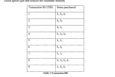
The algorithm will run for all the transactions in the database and the resulting tree

looks as shown in Figure 4.

Figure 4 Complete FP tree

Along with the FP-Tree data structure, this algorithm also maintains item header

table. Each item from that table points to its occurrences in the FP-Tree using

node-links.

Once the FP-Tree construction is complete, mining process starts with the

construction of the conditional pattern base from each frequent 1-itemset. Let us

mine frequent patterns for I3.

I3 has two branches in its conditional FP-tree as shown in Figure 5, which generates

the following set of patterns: {12 13: 4, II 13:2,12 II 13:2}.

Item ID ^U p p o r t Node-Link

. Count . ^ ^ n uu {}

I

L

4

4

_{---- 1 ^}

Figure 5 13 conditional FP Tree

Item

Is

I4

I3

Ii

Conditional pattern base

[(l2li:l),(I2IiI3:l)]

[(I2Ii :l),(l2:l)]

[(I2Ii:2),(I2:2),(Ii:2)]

[(I2:4)]

Conditional FP-tree

(I2:2,1,:2)

(I2:2)

(l2:4,I,:2),(Ii:2)

(I2:4)

Frequent patterns generated

h I5:2,1,15:2,12 I, I5:2

I2 I4:2

I2 I3:4,1,13:2,121,13:2

I2I,:4

Table 11 Frequent Patterns

2.4. Sequential Pattern Mining Algorithms

Sequential pattern mining algorithms were first presented by [AS95]. These algorithms

were based on the apriori algorithms presented by [AS94].

2.5. Apriori ALL

AprioriAll is the first of two algorithms presented by [AS95] to mine sequential patterns.

The essence of this algorithm is to find the maximal sequences. Each such maximal

sequence represents a sequential pattern. A sequence is maximal if it is not contained in

any other longer frequent sequence. This algorithm is based on the Apriori algorithm

presented in [AS94] with the addition of maximal phase that prunes out all non-maximal

sequences. AprioriAll algorithm works on a transformed database, shown in Table 15.

Original customer-sequence database (Table 12) is transformed to a table where

transactions are large itemset (Table 13) which is further replaced by litemset mapping,

as shown in Table 14.

Cust ID

1

Original Cust Seq

[(30) (90)]

Large Itemsets

(30)

Mapped To

2 3 4 5 [(110 20)(30)(40 60 70)]

[(30 .50 70)]

[(30)(40 70)(90)] [(90)] (40) (70) (40 70) (90) 2 3 4 5

Table 12 Customer-sequence Table 13 Large Itemset mapping database Cust ID 1 2 3 4 5

Original Cust Seq

[(30) (90)]

[(110 20)(30)(40 60 70)]

[(30 50 70)]

[(30)(40 70)(90)] [(90)] Transformed Seq [{(30)} {(90)}] [{(30)}{(40),(70),(40 70)}] [{(30), (70)}] [{(30)}{(40),(70),(40 70)}{(90)}] [{(90)}] Mapped Seq [{1}{5}] [{1} {2,3,4}] [{1,3}]

[{1} {2,3,4} {5}]

[{5}]

Table 14 Mapped sequences

Cust ID 1 2 3 4 5 Mapped Seq [{1} {5}] [{1} {2,3,4}] [{1,3}]

[{1} {2,3,4} {5}]

[{5}]

The algorithm finds all the frequent patterns the same way as apriori algorithm does. It

starts by scanning the database to get the support count of each frequent 1-itemset, Table

16. Assuming the user specified support to be 40% or 2 customer sequences, we will get

the L] from Ci, shown in Table 17. We get the C

by doing a self join of Li using

apriori-gen function as described in [AS94]. The algorithm will keep on generating the

candidate itemsets and their corresponding large itemsets unless our candidate itemset

becomes empty and we can not produce anymore large itemsets. Table 18 to Table 23

shows all of the candidate itemsets and large itemsets generated in sequence phase of

AprioriAll algorithm. The maximal phase prunes out all of the non-maximal sequences

from the large sequence sets to give the sequential patterns. Maximal phase uses the

following algorithm to do this task [AS95]

F o r ( k = n ; k > l ; k - ) d o

For each k-sequence Sk do

Delete from S all subsequences of Sk

S is the set of all large sequences generated in sequence phase. The maximal large

sequences (sequential patterns) generated are shown in Table 24.

Seq

(1)

(2)

(3)

(4)

(5)

4

2

4

4

4

Seq

(1)

(2)

(3)

(4)

(5)

4

2

4

4

4

Seq (12 3) (12 4) (13 4) (13 5) (14 5)

(2 3 4)

(3 4 5)

Supp

2

2

3

2

1

2

1

Seq

(12 3 4) (13 5) (4 5) Supp

2

2

2

(123)

(2 3 4)

Supp

2

2

3

2

2

Table 24 Maximal Large Sequences

2.6. AprioriSome

Seq (12 3 4)

Supp

2

Seq (12 3 4)

Supp

2

AprioriSome is also presented in [AS95] along with AS. The main difference between

AprioriAll and AprioriSome is that AprioriAll generates all large sequences, including

non-maximal sequences. Whereas AprioriSome generates large sequences for some and

avoids generating unnecessary non-maximal sequences for the others. AprioriSome has

two phases: forward phase and a backward phase. In the forward phase, it generates all

the large itemsets for certain length sequences. It uses a function next that gives the

length of next sequence to be processed. In backward phase, algorithm counts the

sequences for the lengths that it skipped in the forward phase along with deleting

non-maximal sequences that were found in the forward phase. Taking the same database

sample we used in Table 15 the AprioriSome forward phase will generate the Q , Li, C2,

L2 and C3. It will skip generating the L3 and using the apriori-generate function will

generate the C4 from C3. From C4 it will get the L4. Forward phase will halt here since

sequences from L4. Since the only sequence in L4 is (1 2 3 4), from Table 23, which is

maximal, hence nothing will be deleted from L4. Since we skipped the L3 in forward

phase, in backward we will delete all the subsequences of (1 2 3 4) that are in C3. As a

result, we are left with (1 3 5) and (3 4 5). Since (3 4 5) support count is only 1, it is also

dropped. Going one step back, all sequences from L2 are also deleted except (4 5). At

the end, all of the sequences form the L] will be deleted since all of them are subsets of

the thus far found maximal sequences. Final maximal large sequences are (1 2 3 4) (1 3

5) and (4 5).

2.7. WAP Tree

In the last section we saw apriori like algorithms for mining sequential patterns.

WAP-tree or Web Access Pattern Tree was developed by [PHM+00] for mining the sequential

patterns from web logs in non-apriori like fashion. WAP tree resembles more the FP-tree

algorithm in the sense that WAP Tree also transforms the database into a compact tree

like structure and then employees a mining algorithm on it. WAP-tree uses a WASD,

Web Access Sequence database. WASD is obtained after the first scan of the database is

done and the non-frequent parts of every sequence are discarded. Let us work on an

example of web log sequence shown in Figure 6 as <User ID, Access content>

< 100,a><l 00,b><200,e><200,a><300,b><200,e>< 100,d><200,b><400,a><400,f> <100,a><400,b><300,a><100,c><200,c><400,a><200,a><300,b><200,c><300,f> <400,c><400,f><400,c><300,a><300,e><300,c>

These events are pre-processed in such a way that all access sequences for each user are

grouped together to form a transaction database as shown in Table 25

TID

100 200 300 400

WASD

abdac eaebcac babfaec afbacfc

Table 25 Web Access Sequence Database

After the transformation, dataset is scanned to get the frequency of each event. Assuming

the minimum support of 75%, each sequence in WASD database is transformed into

frequent subsequence as shown in Table 26. The support count for the events is a=4,

b=4, c=4, d=l, e=2 and f=2. Since the support count for d, e and f is less that 75%, they

are dropped from the web access sequences.

TID

100 200 300 400

WASD

abdac eaebcac babfaec afbacfc

Frequent Subsequence

abac abcac babac abacc

Table 26 WASD Frequent Subsequences

Construction of WAP tree starts the same way as of FP-tree. A header node table is

created with frequent events from the frequent subsequences to facilitate the tree

traversal. Lets us now look at the complete construction of the three in following steps.

o A virtual root is created.

(^ Null J

o Each event from the sequence is inserted into the tree as a node with count 1 from

Root if that node type does not exist in that path, but the count is incremented by

o Taking first sequence 'abac' from the Table 26, node with label 'a' will be

inserted as a left child of the Root. Header node table is also updated and event

'a' in the header table is linked to this node. Since there is no immediate child of

the root labeled 'a', we will assign 1 to this node 'a', ' b ' follows 'a' in this

sequence and it will be made the let child of node labeled 'a'. After that we will

insert 'a' as the right child of the node ' b ' . At the end we will insert ' c ' as the

right child of the just created node 'a'. Counter for all these nodes will be set to 1.

Final branch for sequence 'abac' is shown in Figure 7

Item ID Node-Link

/ ^ ^ null {}

a b c

-\ \

\

_ . / V y

U5

( a:l J

•A J

Figure 7 Tree branch for TID 100

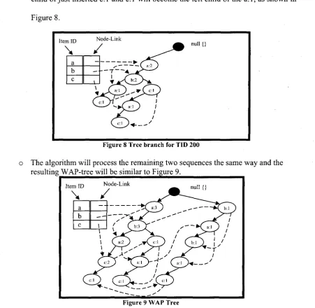
o The second sequence 'abcac' is then processed. Since there is an immediate child

of root with label 'a' exists, algorithm does not insert a new node with label 'a' as

child instead it will increment the count of 'a' to 2. Counter for node with label

'b' will also be incremented by 1 since it also already exists. Since the next node

in the existing path is 'a' which does not match the event ' c ' in this sequence,

child of just inserted c:l and c:l will become the left child of the a:l, as shown in

Figure 8.

Item ID

\ a b c

Node-Link

—

\ \

— T — + - 4 T —

-— ^•C

O '

r CM ^-^ y

A null {}

Figure 8 Tree branch for TID 200

o The algorithm will process the remaining two sequences the same way and the

resulting WAP-tree will be similar to Figure 9.

Item ID Node-Link

\ /

null {}

a

Figure 9 WAP Tree

Completion of the WAP-tree is followed by the WAP-mine algorithm that mines all

frequent sequential patterns from the tree. Following steps are taken to complete the

WAP-mine.

o Mining starts with the lowest entry in the header table which in our example is 'c'

and all the conditional sequence base of c are discovered, i.e. aba:2, ab:l, abca:l,

from the list of conditional sequence base of 'c' because such sequences are

prefix sequences of other sequences. For example, aba and ab have count -1 and

you may notice that aba and ab are prefix sequences of conditional sequence aba.

This deduction is done to avoid these sequences from contributing twice. Now

for these events to qualify as a frequent conditional event, one event must have a

count of at least 3. Getting the counts from the sequences above, we get a:4, b:4

and c:2. Since c:2 is less than the min support of 3, it will be discarded. After

this elimination of 'c', the resulting conditional sequences based on c are aba:2,

ab:l, aba:l, ab:-l,baba:l, aba:l.

o Using the above sequence, algorithm will now generate a conditional WAP tree,

WAP-tree|c as shown in Figure 10.

Item ID \

a b

Node-Link

- -

—/^—4_>^-\ S v

* * / \ b:3 f ^" A a:l ) i

Figure 10 Conditional WAP-tree|c

o New conditional WAP tree is now ready to be mined, as shown in Figure 10.

o Next suffix subsequence be is found as a:3, ba:l and NULL. Since a is the only

frequent event with count 3, 'b' will be discarded and a:4 becomes the frequent

sequence base of 'be'. The recursive re-construction of WAP tree based on be

ends here with c, be and abc as the frequent sequences found so far. The

suffix 'ac' computed from figure 10 is NULL, ab:3, b:l, bab:l, and b:-l. Using

the just mentioned list, algorithm will build the conditional WAP-tree for base

'ac', as shown in Figure 11.

Item ID \

a b

Node-Link /

-C b:3

a:3 \ s ' V b : 1 )

* — '

Figure 11 Conditional WAP-tree|ac

o The algorithm next finds the conditional sequence bases of bac as a:3 and ba:l.

The only frequent sequence from here is a:4. Next the conditional WAP-treejbac

is built with a:4. From here, the algorithm will go back to complete the mining of

suffix ac and starts mining for suffix aac. The only sequence we get from

conditional sequence base aac is b: 1 which is not frequent hence the conditional

search for 'c' ends. The conditional search for events 'a' and ' b ' is also done the

same way as the mining for patterns with suffix 'c' is done.

o The complete frequent pattern set obtained at the end of WAP-mine algorithm is

shown in figure 11.

{c, aac, bac, abac, ac, abc, be, ,b, ab, a, aa, ba, aba}

Figure 12 Complete frequent pattern set

Unlike Apriori-like algorithms that make multiple scans of the databases to mine

generation of candidate sets. But, at the same time, it introduces the construction of large

recursive intermediate WAP-trees during mining process, hence introducing the problem

of efficiently storing and managing the main memory for such intermediate WAP trees.

In the next section we will see how PLWAP algorithm presented by [LE03], [LE05] and

[ELL05] eliminates the construction of such intermediate WAP-trees and improves the

performance of mining sequential patterns.

2.8. SPADE

In [ZOO], the author proposed the SPADE (Sequential PAttern Discovery using

Equivalent Class) algorithm. SPADE uses vertical format sequential pattern mining

technique. In this technique an object is associated with each sequence in which it

occurred along with the time stamp. Sequential pattern mining is implemented by

growing the subsequences using apriori candidate generation. Bottleneck of SPADE is

the generation of huge set of candidate sequences and the multiple scans of database in

mining.

2.9. PrefixSpan

PrefixSpan was introduced by [PJ+01] and it is based on freeSpan. FreeSpan uses

frequent items to recursively project sequences databases into a set of smaller projected

databases and grow subsequence fragments in each projected database. The drawback of

freeSpan is that the algorithm needs to keep the projected sequence in its original

database without length reduction. PrefixSpan on the other hand is a prefix-based

projection algorithm. It examines the prefix subsequence and projects their

candidate sequences and projected databases keeps on shrinking. Major cost of

PrefixSpan is the construction of the project database and storing it in the memory.

PrefixSpan also proposed two projection techniques 1) bi-level projection for reducing

the number and sizes of projected database 2) Pseudo-projection that avoids physical

copying of postfixes by using pointers to form projections.

2.10. PLWAPTree

PLWAP or the Pre-order Linked Web Access Pattern Tree was introduced by [LE03],

[LE05] and [ELL05]. It eliminates the need for recursively re-constructing the

intermediate WAP-trees during mining. It employs binary position code assignment to

the nodes that helps determine the suffix tree for any frequent pattern prefix and

eliminates the need of constructing the intermediate trees. Rule 2.1 from [LE03] defines

the assignment of binary code as

"Given a WAP-tree with some nodes, the position code of each node can simply

be assigned following the rule that the root has null position code, and the

leftmost child of the root has a code of 1, but the code of any other node is derived

by appending 1 to the position code of its parent, if this node is the leftmost child,

or appending 10 to the position code of the parent if this node is the second

leftmost child, the third leftmost child has 100 appended, etc. In general, for the

nth leftmost child, the position code is obtained by appending the binary number

PLWAP or the Pre-order Linked Web Access Pattern Tree was introduced by [LE03],

[LE05] and [ELL05]. It eliminates the need for recursively re-constructing the

intermediate WAP-trees during mining. It employs binary position code assignment to

the nodes that helps determine the suffix tree for any frequent pattern prefix and

eliminates the need of constructing the intermediate trees. Rule 2.1 from [LE03] defines

the assignment of binary code as

"Given a WAP-tree with some nodes, the position code of each node can simply

be assigned following the rule that the root has null position code, and the

leftmost child of the root has a code of 1, but the code of any other node is derived

by appending 1 to the position code of its parent, if this node is the leftmost child,

or appending 10 to the position code of the parent if this node is the second

leftmost child, the third leftmost child has 100 appended, etc. In general, for the

nth leftmost child, the position code is obtained by appending the binary number

of "' to the parent's code ".

There are three main steps of PLWAP algorithm implementation, which are given below.

• Step 1: Frequent-1 events are obtained by scanning the access sequence database.

All events that have support equal or greater than the minimum support are frequent. In

the PLWAP-tree, each node stores node label, node count and node position code. The

root of the tree is a special virtual node with an empty label and count 0.

• Step 2: Database is scanned for the second time to obtain the frequent sequences

from each transaction. The non-frequent events in each sequence are deleted from the

prefix tree data structure, called PLWAP tree, by inserting the frequent sequence of each

transaction in the tree the same way the WAP-tree algorithm would insert them. The

insertion of frequent subsequence is started from the root of the PLWAP-tree. Taking

first sequence 'abac' from Table 26, node with label 'a' will be inserted as a left child of

the Root. Since there is no immediate child of the root labeled 'a', we will assign count 1

to this node 'a' and set its position code by applying Rule 2.1 above. Event ' b ' follows

'a' in this sequence and it will be made the let child of node labeled 'a' with count set to

' 1' and position code set by again using rule 2.1. After that we will insert 'a' as the right

child of the node ' b ' . At the end we will insert ' c ' as the right child of the just created

node 'a'.

Once all of the sequences are inserted in the PLWAP-tree from table 26, the tree is

traversed in pre-order fashion (by visiting the root first, the left subtree next and the right

subtree finally), to create the frequent header node linkage. To assist node traversal

during mining process, auxiliary node linkage structure is constructed. All the nodes in

the tree with the same label are linked by shared-label linkages into a queue, called

event-node queue. The event-event-node queue with label e; is also called ej -queue. There is one

header table for a PLWAP-tree, and the head of each event-node queue is registered.

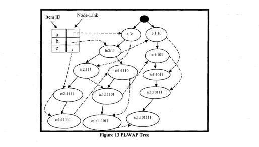
Figure 13 PLWAP Tree

Step 3: mine algorithm uses suffix subsequences to construct intermediate

WAP-trees to find the frequent sequence. PLWAP on the other hand finds the prefix event first

and then uses the suffix tree. Since PLWAP does not create intermediate WAP-trees, it

uses property 2.1 [LE03] to determine quickly if the given node is an ancestor or

descendant of the other node hence finding the suffix tree of a particular event without

reconstructing the intermediate trees. The property 2.1 from [LE03] states

"A node a is an ancestor of another node f3 if and only if the position code of a with "1"

appended to its end, equals the first x number of bits in the position code of p, where x is

the ((number of bits in the position code of a) + I). "

Taking Figure 13 as an example with minimum support of 75%, let us find frequent

• PL WAP Algorithm starts mining with the first element from the header linkage table.

In our example it is 'a'. Following the 'a' link, the first occurrence of 'a' node in the

two suffix trees of the root at a:3:l and b:l :10 is mined. The first occurrence in both

suffix trees is found at node a:3:1 and a: 1:101. Since the sum of counts of both these

nodes is greater than the minimum support, hence 'a' is considered as frequent

1-sequence.

• Next the algorithm will look at 2-sequence that starts with 'a'. The suffix trees of

1:3:1 and a:l:101 rooted at b:3;ll and b:l: 1011 are mined. The first occurrences of

'a' in these suffix trees are found at nodes a : 2 : l l l , a:l: 11101 and a:l: 10111. Since

the frequency count of these node is more than 3 hence 'a' is added to the last list of

frequent sequence 'a' forming 'aa' frequent sequence.

• The algorithm will next mine the suffix trees of nodes mentioned in last step. The

roots of these suffix trees c:2:l 111, c:l:l 11011 and c:l:101 111 will give ' c ' frequent

event to make 'aac' frequent sequence. The last suffix tree is c: 1:11111 which is not

frequent hence terminating the recursive search for 'a' and starts with the next event

'b' from the header linkage table. The algorithm backtracks and finds b:3:ll and

b: 1:1011 and generates ' b ' frequent event giving 'ab' frequent sequence. The

algorithm progresses and finds other frequent sequences with 'ab' as their prefix

sequence i.e 'aba', 'abac' and 'abc'. The algorithm terminates here as no more

frequent sequences are found and backtracks to find frequent sequences that have ' c '

as prefix event. Algorithm finds frequent event ' c ' from c:2;l 111, c: 1:111011 and

c: 1:101111 to give 'ac' as the frequent sequence. This completes finding all the

• The PLWAP algorithm then finds the frequent sequences starting with 'b' and 'c'.

The complete set of frequent sequences found by PLWAP are

{a,aa,aac,ab,aba„abac,abc,ac,b,ba,bac,bc,c}.

2.11. PLWAP1 & PLWAP2

[WP08] introduced PLWAP 1 and PLWAP2 algorithms that are based on WAP and

PLWAP algorithms. In PLWAP1 algorithm implementation, a new header table is

created in every recursive call during mining that links only those nodes that are under

the new root set. With this approach they are avoiding redundant node checking. In

PLWAP2 algorithm, no new header table is created but the algorithm filters out events

that are not under the new roots. This filtering is achieved by traversing from the new

3. Position Coded Pre-Ordered linked WAP-Tree Long

(PLWAPLongl & PLWAPLong2)

3.1. Problem addressed

We have identified two problems that degrade the PLWAP algorithm performance.

Problem #1: In previous chapter we saw that PLWAP eliminates the need to generate

intermediate conditional WAP trees by first assigning the position codes to each node and

then identifying quickly if a node on a current suffix tree set belongs to a different subtree

so that its count can contribute to the total support count of root set. PLWAP algorithm

implementation represents binary position code of each node by storing its binary code in

a linked list data structure. However, for very long sequences exceeding thirty two

nodes, the number of bits an integer position code can hold, the PLWAP algorithm's

performance begins to degrade because the linked list traversals slow down the algorithm

both during tree construction and mining [ELL05]. This is because when the algorithm

starts the mining process and needs to test the ancestor-descendant relationship of two

nodes, it will first retrieve the complete position code of these nodes by following the

linked lists associated with each one of them. If these nodes happen to be part of the tail

of a very long (more than 32 items) sequence, the retrieval of position codes becomes

slow because the linked list will need to make too many memory reads to traverse

completely through the linked list.

Problem #2: Second problem seen in the PLWAP algorithm implementation is that

during construction of the suffix trees the ancestor-descendant relationship check

unnecessary checks. This is because all events, with the same label, that are ancestor of

event for which suffix tree is being explored, should not be tested for this relationship as

they will never be counted in the suffix tree support. Similarly, those events, with the

same labels, that are descendants of event for which suffix tree is being explored, should

not be included in the support count of the suffix tree as well [LE03]. When dealing with

long sequences where branches have hundreds of event nodes having repeated events, the

algorithm will do many relationship checks just to ignore their support count. This

support check affects the performance when we have very long sequences. From

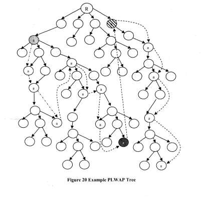
Figure-12 we can see that when algorithm starts the mining process with "root" node in the root

set and event queue 'a', node "a:3:l" is the first node from the event queue 'a' found to

be the first descendant of root and added to the new root set. Although all the

descendants of this node "a:3:l" will be checked for ancestor-descendant relationship but

their counts will not be added, hence taking up time and costing the performance

especially when we have large sequences.

3.2. Proposed solution

To address the problems identified in previous section, we are proposition two new

algorithms, i.e. PLWAPLongl and PLWAPLong2. Both of these algorithms share same

solution for problem #1. To address problem #2, PLWAPLongl algorithm proposes the

transformation of linked list based PLWAP tree into its equivalent array based

representation and employing binary search to find the descendents during root set

creation. On the other hand, PLWAPLong2 algorithm uses the same linked list base tree

technique called 'Last Descendant' to eliminate unwanted node comparisons during root

set creation.

Solution for problem #1: To overcome the first problem, we are proposing a new

position code numbering scheme. Our approach uses two new labels instead of one for

each node i.e. 'startPosition' and 'endPosition' and assigns the numeric values to these

labels during transformation of linked list tree into array based tree with pre-order

traversal of the PLWAP-tree. Along with the assignment of new position code, we are

also proposing the following rule that will be used during the mining process to

determine the ancestor-descendant relationship of any two nodes.

Rule 1.0

"Given two nodes, n\ and n2, nj is ancestor of n2 (or n2 is descended of nj) if

nj.startPosition < n2.startPosition & if'«;.endPosition > n2.endPosition".

In subsequent section we will discuss both new algorithms in detail and discuss how to

address problem #2.

3.2.1. PLWAPLongl

Solution of problem #2: To address the second problem identified in section 3.1, we are

proposing the following new processing:

1. Transform the PL WAP tree to its equal Array representation.

2. Maintain the position of the last descendant of each event.

3. Employ binary search to find the immediate descendant during root set creation.

Here is how rest of this chapter is organized. Section 3.2.1 details the new approach of

transforming the linked list based PLWAP tree to its equivalent array based

3.2.3 details the importance of using binary search to find immediate descendant. Section

3.2.4 presents the mining algorithm for PLWAP-Long with example. Section 3.2.5

outlines PLWAPLongl, transformTree and buildDesc algorithms.

3.2.1.1. Array Representation

The reason for transforming the linked list tree to its equivalent array representation is

that with arrays we can jump from one node to the other known node in a 0(1) time. In

case of linked list based PLWAP-tree, memory references of parent, child and sibling are

stored in nodes and memory seek is required in order to obtain the actual address.

Another advantage of array representation is that we do not need to chain the same label

events as we did in the linked list tree because during transformation event arrays are

constructed using the pre-order traversal of the linked list tree and hence all events with

same label are inserted in their respective event arrays in ascending startPosition. Once

all of the events with same label are inserted in their respective event arrays, starting from

index 0 and incrementing the index by 1 will explicitly chain these same label events.

The header table is also represented using array of linkheader structure.

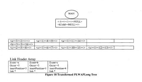
Note: To keep the transformed array based PLWAP-Long tree figures simple, all of the

values a node holds are shown within <>. The order of these values is

<event><occur><startPosition><endPosition><lastDesc>.

Taking the Figure-13 as example, let us transform the tree to its array representation

using pseudo code of transformTree algorithm shown in Figure 21. A new method

transformTree() is called that takes in root node of the linked list tree, NULL parent node

and NULL leftChild node. transformTree method traverses through the linked list tree in

the startPosition and the endPosition. It starts with the event of the root node and looks

up the header table array and finds the event.

Since it is the start of the transformation and the fact that root event has label - 1 , we

won't find this event in the header table and hence create a new root node. startPosition

' 1 ' is assigned to the root node. This root node will point the transformed array

represented tree. Following the algorithm from Figure-21, we will call the transform tree

method with left child of the root (i.e. a:3:l), the newly created root and the NULL (since

the newly created root has not yet assigned the left child). Note: The link header array

is populated when the original linked list PL WAP tree is constructed. The event arrays

are also dynamically created at this very moment and start of each array is linked to the

event entry in the link header array. In this example from Figure-13, three event arrays

will be created for event 'a' size 5, event 'b' size 2 and event 'c' with size 5. Algorithm

will find the array index of this event from the link header array, i.e. 0, and also retrieve

the insertPosition. InsertPosition gives the location where new node should be inserted

within that event array. Since this is the first time event 'a' is seen, this node will be

inserted at position 0, as shown in Figure 14.

( ROOT )

<-1 > o < 1 ><><NULL> <lChild><NULL><>

Link Header Array

Event =a Occur =5 insertPosition=l link *

Event=b Occur =3 insertPosition=0 link*

Event=c Occur =5 insertPosition=0 link *

Next we get the left child of this event which is b:3:ll and insert it into the event array

'b' pointed by the link header array index 1. Since this is the first time event b is

recorded, the inserfPosition is set to 0 and hence b:3:ll will be inserted at position 0 in

the event array 'b' as seen in Figure 15. We will keep on traversing in the pre-order

fashion until we get to the last event in leftmost branch of the original tree. The array

values at that point will be as shown in Figure 16.

ROOT

<-1 > o < l > < > < N U L L > <lChild><NULL>o

<a><3><2><><> <b><3><3><><>

Link Header Array

Event =a Occur =5 insertPosition=l link* Event=b Occur =3 insertPosition=l link * Event=c Occur =5 insertPosition=0 link *

Figure 15 Transformed PLWAPLong-Tree with node b:3:ll

f ROOT A

<-1 > o < 1 ><><NULL> <lChild><NULL>o <a><3><2><><> <b><3><3><><> <c><2><5><><> <a><]><4><><> <c><1><6><7><>

Link Header Array

Event =a Occur =5 insertPosition=2 link * Event=b Occur =3 insertPosition=l link * Event=c Occur =5 insertPosition= link * =2