2018
Buckling Effect on the Performance of Solar Cells under Different
Buckling Effect on the Performance of Solar Cells under Different
Loading Conditions
Loading Conditions
Ahmed Alateeq
Iowa State University, [email protected]
Follow this and additional works at: https://lib.dr.iastate.edu/creativecomponents
Part of the Structural Engineering Commons
Recommended Citation Recommended Citation
Alateeq, Ahmed, "Buckling Effect on the Performance of Solar Cells under Different Loading Conditions" (2018). Creative Components. 23.
https://lib.dr.iastate.edu/creativecomponents/23
Ahmed Alateeq
A creative component submitted to the graduate faculty
in partial fulfillment of the requirements for the degree of
MASTER OF SCIENCE
Major: Civil Engineering (Structural Engineering)
Program of Study Committee: An Chen, Major Professor
In Ho Cho Ashley Buss
Iowa State University
Ames, Iowa
2018
TABLE OF CONTENTS
ABSTRACT ... xi
CHAPTER 1. INTRODUCTION ... 1
1.1 BACKGROUND ... 1
CHAPTER 2. PERFORMANCE OF SOLAR CELLS INTEGRATED WITH RIGID AND FLEXIBLE SUBSTRATES UNDER COMPRESSION ... 5
2.1 MATERIAL PROPERTIES ... 5
2.1.1 SOLAR CELL PROPERTIES ... 5
2.1.2 FIBER RIENFORCED POLYMER (FRP) PROPERTIES ... 5
2.1.3 CONCRETE PROPERTIES ... 6
2.1.4 THIN FRP PROPERTIES ... 6
2.2 SPECIMEN FABRICATION ... 7
2.2.1 FRP Fabrication ... 7
2.3 TESTING SETUP ... 9
2.3.1 Confined, Wrapped FRP, and Normal Concrete Cylinders ... 9
2.3.2 Neoprene Rubber ... 10
2.3.3 Thin FRP ... 11
2.4 TESTING RESULTS ... 12
2.4.1 Confined, Wrapped FRP, and Normal Concrete ... 12
2.4.2 Thin FRP ... 23
2.4.3 Neoprene Rubber ... 26
2.5 BUCKLING EFFECTS ... 32
2.6 DISCUSSION AND CONCLUSIONS ... 38
CHAPTER 3. PERFORMANCE OF SOLAR CELLS INTEGRATED WITH CONFINED FRP REINFORCED CONCRERTE UNDER FLEXTURAL TEST ... 39
3.1 MATERIAL PROPERTIES ... 39
3.1.1 Concrete Properties ... 39
3.1.2 Steel Reinforcement ... 39
3.2 MATERIAL FABRICATIONS ... 41
3.2.1 FRP Fabrication ... 41
3.2.2 Strain Gauge Installation ... 43
3.3 TESTING SETUP ... 47
3.3.1 Three Point Loading Flexural Testing... 47
3.4 TESTING RESULTS ... 49
3.4.1 Three-Point Loading Flexural Testing ... 49
3.4.2 Evaluating Amorphous Silicon Solar Cells under Compression ... 50
3.4.3 Evaluation of Compression Specimens (Solar Cell under Compression) under Flexural Test ... 54
3.4.4 Failure Modes of Solar Cell under Compression Specimens ... 59
3.4.5 Evaluating Amorphous Silicon Solar Cells of the Solar Cell under Tension Specimens ... 60
CONCRETE BEAM WITH FRP CONFINED ... 70
4.1.1 Inelastic Properties of Concrete ... 71
4.1.1.1 Concrete Compressive Behavior ... 71
4.1.1.2 Concrete Tensile Behavior ... 75
4.1.1.3 Steel Tensile Behavior ... 77
4.1.2 Simulation of Solar Cell under Compression Specimens ... 79
4.1.3 Mesh Convergence Study ... 81
4.1.4 Validation the Results of Solar Cell under Compression Specimens with FE Simulation ... 83
4.1.5 Validation the Results of Solar Cell under Tension Specimens with FE Simulation ... 85
REFERENCES ... 89
LIST OF FIGURES
Figure 1-1 JV- Curve of silicon solar cell under high temperatures…………...……2
Figure 1-2 Temperature dependence of MPP………...…2
Figure 1-3 Light intensity dependence of MPP………...……….….2
Figure 1-4 JV-Curves of silicon solar cell under different light intensity…...3
Figure 2-1 (SP3-12) solar cell configuration ... 5
Figure 2-2 Thin FRP plate. ... 6
Figure 2-3 (a) aluminum mold, (b) fabricated FRP with aggregate, (c) aluminum roller ... 8
Figure 2-4 Wrapped FRP concrete. ... 8
Figure 2-5 Keithley 2400 SourceMeter, and Labview... 9
Figure 2-6 SATEC Machine. ... 9
Figure 2-7 confined concrete specimen under the illumination of the projector. ... 10
Figure 2-8 Hard Multipurpose Neoprene Rubber Cylinder. ... 11
Figure 2-9 (a) Compression Test set-up, and (b) Thin FRP specimen with compressible springs. ... 12
Figure 2-10 Strain-Stress Curve of Normal Concrete Specimens ... 13
Figure 2-11 Strain-Stress Curve of FRP Confined Concrete Specimens. ... 13
Figure 2-12 Strain-Stress Curve of Wrapped FRP Concrete Specimens ... 14
Figure 2-13 J-V characteristics curves of Normal Concrete (Specimen 1). ... 15
Figure 2-14 J-V characteristics curves of Concrete with FRP Confined (Specimen 2). ... 16
Figure 2-15 J-V characteristics curves of Concrete with Wrapped FRP (Specimen 1). ... 16
Figure 2-16. Solar Cell IV- Characteristic Curve (Alternative Energy Tutorial). ... 17
Figure 2-17. Fill Factor (FF) physical meaning (National Instruments) ... 18
Figure 2-20 MPP vs. strain for Wrapped FRP- concrete specimens. ... 19
Figure 2-21(a) FRP-confined concrete (Before), and (b) FRP-confined concrete (After). ... 21
Figure 2-22 (a) Solar cell failure of normal concrete; (b) Strain gauge failure of normal concrete; (c) Solar cell failure of FRP-confined concrete with aggregate; (d) Strain gauge failure of FRP-confined concrete with aggregate; (e) FRP failure of FRP-confined concrete. (f) Wrapped FRP concrete Failure. ... 22
Figure 2-23 Load-Vertical Displacement Curve of Thin FRP. ... 23
Figure 2-24 JV Curves of Thin FRP (Specimen 1)... 24
Figure 2-25 JV Curves of Thin FRP (Specimen 3)... 24
Figure 2-26 MPP vs. Strain of Thin FRP Specimens. ... 25
Figure 2-27 (a) Initial buckling mode. (b) Maximum buckling mode. ... 26
Figure 2-28 Load- displacement Curve of Neoprene Rubber Specimen 1 (Flat). ... 26
Figure 2-29 J-V characteristics curves of Neoprene Rubber (Flat Solar Cell) (Specimen 1). ... 27
Figure 2-30 J-V characteristics curves of Neoprene Rubber (Flat Solar Cells) (Specimen 2). ... 28
Figure 2-31 MPP vs. Displacement of Flat amorphous Solar Cell Specimens. ... 28
Figure 2-32 Local Buckling of Flat Solar Cell (Specimen 2). ... 29
Figure 2-33 J-V characteristics curves of Neoprene Rubber (Curved Solar Cells) (Specimen 2). ... 30
Figure 2-34 J-V characteristics curves of Neoprene Rubber (Curved Solar Cells) (Specimen 3). ... 30
Figure 2-35 MPP vs. Displacement of Curved amorphous Solar Cell Specimens. ... 31
Figure 2-36 Area under Curved Solar Cell. ... 35
Figure 3-1 Steel Reinforcement and concrete cover ... 40
Figure 3-3 Steel Reinforcement at tension side (Concrete). ... 40
Figure 3-4 (a) Oil Spread on the Formwork. (b) Nylon ply Sheet and Solar Cell. ... 41
Figure 3-5 (a) Aluminium Clips and the Aggregates. (b) Poured Concrete. ... 42
Figure 3-6 Final FRP Confined beam specimens ... 43
Figure 3-7 Exceeded height at both FRP sides. ... 43
Figure 3-8 (a) Grinding Machine. (b) smoothed surface of concrete ... 44
Figure 3-9 Placement of glue. ... 44
Figure 3-10 Strain Gauge Configuration (60 mm). ... 44
Figure 3-11 Optimal locations of strain gauges (Solar cell subjected to Compression). ... 45
Figure 3-12 Optimal locations of strain gauges (Solar cell subjected to Tension). ... 45
Figure 3-13 Strain Gauges Placed on FRP Layer (5 mm gauge length)…...46
Figure 3-14 Optimal locations of strain gauges (Solar cell subjected to Compression...46
Figure 3-15 Optimal locations of strain gauges (Solar cell subjected to Tension)...46
Figure 3-16 (a) Test Set-up of Solar cell under Compression (b) Test Set-up of Solar cell under Tension. ... 47
Figure 3-17 (a) Test-Set-Up of Solar Cell under Compression Specimen (b) Four Deflection Transducers ... ...48
Figure 3-18 (a) Data Acquistion Systems (DAQ) (b) Source meter and Labview ...49
Figure 3-19 J-V curves of Flat silicon Solar Cell under Compression (Specimen 1)...50
Figure 3-20 J-V curves of Flat silicon Solar Cell under Compression (Specimen 1)...51
Figure 3-23 Shifted Silicon Solar Cell………...……….. 52
Figure 3-24 Curved Solar Cell near to the Applied Load ...53
Figure 3-25 Load-deflection Curve of Solar Cell under Compression Specimens at Mid-Span. ... ..54
Figure 3-26 Load-deflection Curve of Solar Cell under Compression Specimens under Load (West). ... ...55
Figure 3-27 Load-deflection Curve of Solar Cell under Compression Specimens under Load (East). ... 55
Figure 3-28 Load-strain Curve of Solar Cell under Compression at Mid-Span (FRP) .... 57
Figure 3-29 Load-strain Curve of Solar Cell under Compression at Mid-Span (Concrete) ... 58
Figure 3-30 (a) Debonding of FRP under Load (b) Crack of Concrete (c) Debonding of FRP at the Mid-Span (d) Crack under the applied load (e) Crack Passed Strain gauge (f) Debonding of FRP at both sides………...…...……59
Figure 3-31 JV Curves of Flat Silicon Solar Cell under Tension (Specimen 1)... 61
Figure 3-32 JV Curve of Curved Silicon Solar Cell under Tension (Specimen 1)... 61
Figure 3-33 MPP vs. West deflection of Flat Solar Cells. ...62
Figure 3-34 MPP vs. West deflection of Curved Solar Cells. ... 62
63Figure 3-35 Pre-buckled Shape of the second specimen. ... 63
Figure 3-36 Test Set-up of the Tension Specimens. ... 64
Figure 3-37 Load-deflection Curve of Solar Cell under Tension at Mid-Span. ... 65
Figure 3-38 Load-deflection Curve of Solar Cell under Tension at West direction. ... 65
Figure 3-39 Load-deflection Curve of Solar Cell under Tension at East direction. ... 65
Figure 3-40 Load-strain Curve of Solar Cell under Tension at Mid-Span (FRP) ... 67
Figure 3-42 Crack Started at Top of the concrete ... 69
Figure 4.1 Compressive Stress-Strain Relationship for ABAQUS………..………72
Figure 4.2 Response of Concrete to Uniaxial Loading in Tension………...……….75
Figure 4.3 Modified Tension Stiffening Model………..…….76
Figure 4.4 Stress-Strain Curve of all Three Steel Specimens………..78
Figure 4.5 FE Simulation of Solar Cell under Compression Specimens……….……80
Figure 4.6 FRP Material and Steel rebars in ABAQUS……….…….…….80
Figure 4.7 Stress (Mises) vs. Mesh sizes………...………..82
Figure 4.8 Displacement (Y-axis) vs. Mesh sizes………82
Figure 4.9 Deformed Shape of the Solar Cell under Compression Specimens………...……83
Figure 4.10 FE vs. Experimental Results of Solar Cell under Compression Specimens..…..84
Figure 4.11 Damage location (Red Region)………..………..85
Figure 4.12 Deformed Shape (FRP on Tension Stress)………...85
Table 2-1 Amorphous Silicon Solar Cell Mechanical Properties. ... 5
Table 2-2 Solar Cell Electrical Properties. ... 5
Table 2-3 FRP and Resin Properties (Yossef 2017). ... 6
Table 2-4 Mix Design of Concrete. ... 6
Table 2-5 Thin FRP physical properties. ... 7
Table 2-6 Thin FRP mechanical properties. ... 7
Table 2-7 Average strength and standard deviation ... 14
Table 2-8 Solar Cell Parameters and the Test Results (Thin FRP Specimen # 1) ... 36
Table 2-9 Calculations of Ac, and Relative Efficiency (Thin FRP Specimen # 1). ... 37
Table 3-1 Average strength and standard deviation (Yossef 2017). ... 39
Table 3-2 Average strength and standard deviation (before Testing the Specimens). ... 50
Table 4.1. Material Properties………...………….71
Table 4.2 Concrete Compressive Behavior………..………..74
Table 4.3 Concrete Tensile Behavior……….77
ACKNOWLEDGMENTS
All praise due to Allah (God) for what I have achieved which would not be possible
without his guidance.
I would like to thank Dr. An Chen, for his generous advice, support, and motivation
during my MS study, and my committee members, Dr. In Ho Cho, and Dr. Ashley Buss, for
their guidance, support throughout the course of this research, and serving on my POS
committee
In addition, special thanks for Dr. Mostafa Yossef who provided and assisted me
during the solar cell testing. I would also like to thank Dr. Simon Laflamme and Austin
Downey for allowing me to use the test equipment.
I would also like to thank Douglas Wood and Owen Steffens for their great help in
preparing the testing set-up, and for their support in the lab.
I would also like to thank David Morandeira and Yinglong Zhang for their great help.
I would also like to thank my friends Mohammed Bazroun, Connor Schaeffer, Hao Wu,
colleagues, the department faculty and staff for making my time at Iowa State University
a wonderful experience.
I would also like to thank Qassim University, for their financial support along my MS
Renewable solar energy has been increasingly used due to its efficiency and
cleanliness. Currently, mounting systems are needed to install solar cells on the surface of
supporting structures, such as building roofs. Attaching solar cells directly to the supporting
structures can eliminate the mounting systems and reduce the cost. Once the mounting system
is eliminated, solar cells become an integral part of the supporting structures and they are
subjected to the same strains as those of the supporting structures, Therefore, it is necessary to
study the performance of solar cells under different strain states.
The main objectives of this study are to investigate the possibility of attaching the
amorphous silicon solar cell directly to the supporting systems, and to study the buckling effect
on the amorphous silicon solar cell and their relative efficiency. (Chen et al. 2018) attached
solar cells to fabricated FRP materials to study the effect of strain on the performance of solar
cells under both compression and tension tests. They found that the performance of solar cells
in both cases has a little degradation. The factor behind this degradation, whether it is caused
by the failure of the specimen or from buckling, needs to be investigated. To this end, the solar
cells were attached to different supporting systems (rigid and flexible) to determine the
dominant factor affecting the degradation. Since the amorphous silicon solar cells are attached
to supporting systems, which are subjected to different loads, such as compression, tension,
and flexural loads based on their functions, it is also necessary to investigate the solar cell
under different loading conditions. Therefore, different loads scenarios in addition to different
CHAPTER 1. INTRODUCTION
1.1BACKGROUND
Solar energy is clean and efficient. It has been widely used; especially in the area where
electricity grid is not accessible. In the US, the Solar Investment Tax Credit (ITC) has
successfully pushed hardware prices down and installer experience up. For example, the cost
of solar electricity has decreased from $7.24/W in 2010 to $2.80/W in 2017 for residential
applications (inflation adjusted), mostly due to the cost reduction of the photovoltaic (PV)
module (Fu et al. 2017). Although the price of the module will continue to decrease, there is
little room for substantial reduction. Therefore, more efficient ways are required to optimize
the cost such as eliminating the mounting system (Yossef, 2017). Once the supporting system
is eliminated, solar cells become an integral part of the supporting structures and they are
subjected to the same strains as those of the supporting structures, which are caused by different
types of load, such as gravity, wind, seismic loads, etc.
Extensive research has been conducted to evaluate the performance of silicon solar
cells under different environmental conditions, such as temperature, light intensity, and their
effects on the solar cell parameters (Tobnaghi et al. 2013). It was concluded that the
open-circuit voltage reduced significantly under high temperature with about 2.2 mV/oC, when the
short-circuit current increases slightly with temperature with about 0.0006 mA/ oC as shown in
Figure 1-1 JV- Curves of silicon solar cell under high temperatures (Tobnaghi et al. 2013).
Fill Factor (FF) also decreases when the temperature increases by about 0.0015 / oC,
thereby decreasing the maximum output power (MPP) to 0.005 mw/ oC, and the opposite
occurred when subjecting to high light intensity as shown in Figure 1-2, and 1-3 respectively.
The effect of light intensity on the silicon solar cell parameters was also investigated. It was
concluded that short-circuit current (Isc) is directly proportional to light intensity. As the light
intensity decreases, the Isc decreases and vice versa as shown in Figure 1-4. The efficiency of
the amorphous silicon solar cell decreases as the temperature increases by about 0.25%/ 1oC
compared to 0.4-0.5% /1oC in case of the crystalline silicon solar cells (Zhao et al. 2011).
Figure 1-2 Temperature dependence of MPP. Figure 1-3 Light intensity dependence of MPP.
Figure 1-4 JV-Curves of silicon solar cell under different light intensity (Tobnaghi et al. 2013).
The energy conversion efficiency of amorphous silicon solar cells were about 2.4%
when they first invented by Carlson and Wronski in 1976. The efficiency of amorphous silicon
solar cells is improved to exceed 15%. In 2002, the total output power generated from the
amorphous silicon solar cells was 35.8 MW (Shah 2012).
Extensive research has been conducted to evaluate the performance of solar cells under
tension. Mono-crystalline silicon solar cells were attached to Carbon Fiber-Reinforced
Polymer (CFRP) composite materials using EVA (ethylvinyl acetate) film and tested them
under tension. The performance of solar cells was evaluated using I-V curves. It was concluded
that the performance of solar cells degraded due to cracks on the surface of and inside the solar
cells (Kim and Cheong 2014). Tension test was conducted on amorphous silicon solar cells
and measured their Maximum Power Point (MPP) and Fill Factors (FF). It was concluded that
compression. Amorphous silicon solar cells were attached to FRP materials to study the effect
of strain on the performance of solar cells under both compression and tension (Chen et al.
2018). It was found that, in the tension test, there was little degradation until the failure
happened. However, in the compression test, the solar cells degraded at about 0.5% strain.
(Hamid Saadatmanesh 1991) conducted an experiment on five rectangular specimens
reinforced beams that were strengthening with epoxy bonded glass-fiber-reinforced-plastic
(GFRP) plates placed on the bottom surface of the concrete under third bending point test.
They concluded that the flexural strength increases significantly and the (GFRP) reduces crack
size (Hamid Saadatmanesh 1991). GFRP has many advantages in structural applications
compared to conventional materials. These advantages include excellent resistance to
electrochemical corrosion, and high strength. Furthermore, GFRP is versatile which can be
fabricated in any shape.
(Al-Sulaimani et al. 1994) conducted an experiment on simply supported reinforced
beams that have different configurations including wrapping fiberglass on the sides of the
specimens under four-point loading test. The damage was induced and the beams’ specimens
were designed to fail in shear before attaching the wrapped fiberglass. They concluded that the
CHAPTER 2. PERFORMANCE OF SOLAR CELLS INTEGRATED WITH RIGID AND FLEXIBLE SUBSTRATES UNDER COMPRESSION
2.1 MATERIAL PROPERTIES
2.1.1 SOLAR CELL PROPERTIES
Solar cells used in the experiment were amorphous silicon thin-film solar cells
(SP3-12) manufactured by Power Film Solar, as shown in Figure 2.1. Tables 2.1 and 2.2 list
mechanical and electrical properties provided by the manufacturer.
Table 2-1 Amorphous Silicon Solar Cell Mechanical Properties.
Height (mm) Length (mm) Width (mm) Weight (g) Aperture Size (mm2)
0.2 63.5 12.7 0.34 12.7 x 50.8
Table 2-2 Solar Cell Electrical Properties.
Wattage (W) Voltage (V) Voltage (Voc)
(V) Current (mA)
Short-Circuit Current (Isc) (mA)
0.0255 3.0 4.5 8.5 10.7
2.1.2 FIBER RIENFORCED POLYMER (FRP) PROPERTIES
The type of the FRP material used in the experiment was Chopped Stand Mat, and the
404-isophthalic resin used as an epoxy to fabricate the FRP layer according to (Petersen et al.
Figure 2-2 Thin FRP plate.
Material Material type
Tensile Strength
(MPa)
Tensile Modulus
(GPa)
Compressive Strength
(MPa)
Density (g/cm3)
E-Glass Fiber Chopped Strand Mat 2000 72.4 -- 2.56
Resin 404 Isophthalic Resin 503.3 36.5 82.73 1.1
2.1.3 CONCRETE PROPERTIES
Concrete used in the experiment as a rigid substrate where the solar cell was attached.
The type of the concrete was Portland Cement Concrete that was ordered from Polk County,
Iowa. The concrete mix design is given in table 2.4.
Table 2-4 Mix Design of Concrete.
Cement
(kg/m3) Fly Ash (kg/m
3) Water (kg/m3) Fine Aggregate
(kg/m3)
Coarse Aggregate (kg/m3)
2,107 314 1,000 6,666 6,741
2.1.4 THIN FRP PROPERTIES
Thin FRP plate (0.003 in. thickness) used in this experiment as a flexible substrate,
which was attached with solar cells and strain gages as shown in Figure 2.2. Physical and
Table 2-5 Thin FRP physical properties.
Table 2-6 Thin FRP mechanical properties.
Tensile Strength (MPa) Compressive Strength (MPa) Flexural Strength (MPa)
68.9 220.6 160.0
2.2 SPECIMEN FABRICATION
2.2.1 FRP Fabrication
The FRP described in section 2.1.2 was used as the confined material of the concrete
cylinders. Two different manufacturing process were used to confine the concrete cylinders.
First, a mold of circular aluminum metal (4 in. x 8 in.) with a cut off into two parts. The two
parts are combined together using a ring. A Nylon Release Peel Ply was used to confine the
inner diameter of the circular mold to easily release the FRP after being fabricated. Then the
solar cell was attached to the Nylon Release Peel Ply in the middle of the cylinder. After that,
the FRP was inserted inside the mold. The FRP fabrication was divided into three stages. In
each stage, the 404 Isophthalic Resin was distributed above the FRP and an aluminum roller
used to squeeze the epoxy on the surface of the FRP. Eventually, the aggregate was added on
the surface to ensure a strong bond between the FRP and concrete. Figure 2.3 (a, b, and c)
show the aluminum mold, fabricated FRP, and aluminum roller.
Material Type Grade Length (mm) Width (mm) Thickness (mm)
Figure 2-3 (a) aluminum mold, (b) fabricated FRP with aggregate, (c) aluminum roller
(a) (b) (c)
Second, the FRP was wrapped around the concrete cylinder after the concrete achieves
its fully strength. The Nylon Release Peel Ply was used as a cover, where the amorphous silicon
solar cell was attached. The FRP was placed on the Nylon Release Peel Ply, and then the 404
Isophthalic Resin was applied to the FRP and an aluminum roller used to distribute the resin.
After that, the concrete cylinder was used as a roller to wrap the FRP. Figure 2.4 shows the
wrapped FRP concrete.
Figure 2-6 SATEC Machine. Figure 2-5 Keithley 2400 SourceMeter, and Labview. 2.3 TESTING SETUP
2.3.1 Confined, Wrapped FRP, and Normal Concrete Cylinders
The confined and wrapped FRP, and Normal Concrete Cylinders with a dimension of
4 in. (diameter) and 8 in. (height). They were tested under compression load using the SATEC
Machine at ISU. In case of the confined and wrapped FRP, the solar cell was attached directly
to the FRP during the fabrication process, but in case of normal concrete, the solar cell was
attached directly to the concrete as a rigid substrate after it achieved its fully strength. The
objectives of this experiment is to investigate the possibility of directly attaching the solar cell
to the supporting system, i.e., eliminating the mounting system.
Strain gauges were installed on each specimen. The load, displacement, and strain data
were measured using the SATEC Machine as shown in Figure 2.5. Keithley 2400 SourceMeter
was used to connect the solar cell to obtain the I-V characteristics curves through a four wires
connection as shown in Figure 2.6. A lab view software created by (Elshobaki 2015) was used
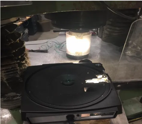
Figure 2-7 confined concrete specimen under the illumination of the projector. projector. (Sugar et al. 2007) proved that the quantum efficiency peaks of the solar cell is
around 540 nm, which is within the projector spectrum. This projector was calibrated to
simulate 100% sunlight. To be consistent in the experiment, the distance between the solar cell
and the light source was the same for all specimens. Figure 2.7 shows the confined concrete
specimen under the illumination of the projector. During the experiment, J-V curves, Fill
Factor (FF), Short Current Circuit (Isc), Open Voltage Circuit (Voc), and other parameters were
measured.
2.3.2 Neoprene Rubber
The type of the rubber used in this experiment was Hard Multipurpose Neoprene
Rubber Rod as shown in Figure 2.8. The Neoprene Rubber was tested under compression load
using the SATEC Machine at ISU. This rubber allows larger deflection of the specimen when
subjected to compression load, in addition to its applicability in Civil Engineering. The
Figure 2-8 Hard Multipurpose Neoprene Rubber Cylinder.
same procedures as those for normal concrete were used for Neoprene Rubber in terms of
testing set-up and attaching solar cells.
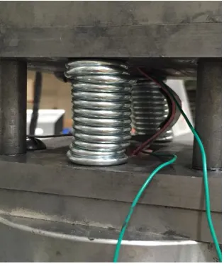
2.3.3 Thin FRP
Five specimens of solar cell attached to flexible FRP substrate were tested under
compression using an MTS machine as shown in Figure 2.9 (a) at a loading rate of 7.62
mm/min. As the loading rate increases, the buckling of the thin FRP will form quickly. The
compression fixture developed by (Barbero et al. 1999) was used in the experiment to allow
for the light source produced by A Kodak Carsoul 750H with DEK 500W projector to reach
the specimens. Since the FRP substrate was flexible, two compressible springs were added
between the upper and lower plates of the compression fixture to avoid the fracture of specimen
caused by excessive displacement, as shown in Figure 2.9 (b). Load, displacement, and strain
Figure 2-9 (a) Compression Test set-up, and (b) Thin FRP specimen with compressible springs. (a) (b)
2.4 TESTING RESULTS
2.4.1 Confined, Wrapped FRP, and Normal Concrete
The normal, confined FRP, and wrapped FRP concrete cylinders were tested under
compression using SATEC machine. Strain gauges were attached to each specimen. During
the test process, the current was recorded as the voltage changes because of the applied load at
different magnitude of displacements. Then the load, strain data were collected from the DAQ
as described previously. Eight specimens were tested with four specimens for each group.
The strain-stress curves of normal, confined FRP, and wrapped FRP concrete cylinders
specimens were obtained as shown in Figure 2.10, 2.11, and 2.12 respectively. From the data
provided in the strain-stress curves, the average strength of all concrete specimens, and
0 1000 2000 3000 4000 5000 6000 7000 8000 9000
0 500 1000 1500 2000 2500 3000
S tr ess (ps i) Strain (με)
Normal Concrete 1 Normal Concrete 2 Normal Concrete 3 Normal Concrete 4
[image:25.612.129.484.107.370.2]Figure 2-10 Strain-Stress Curve of Normal Concrete Specimens
Figure 2-11 Strain-Stress Curve of FRP Confined Concrete Specimens. 0 1000 2000 3000 4000 5000 6000 7000 8000
0 1000 2000 3000 4000 5000
S tr ess (psi ) Strain (με)
FRP Confined Concrete Specimen 1
FRP Confined Concrete Specimen 2
0 1000 2000 3000 4000 5000 6000 7000 8000 9000 10000
0.00 500.00 1000.00 1500.00 2000.00 2500.00
S
tr
ess
(psi
)
Strain (με)
Wrapped FRP Concrete 1
Wrapped FRP Concrete 2
Wrapped FRP Concrete 3
Figure 2-12 Strain-Stress Curve of Wrapped FRP Concrete Specimens
Table 2-7 Average strength and standard deviation
Specimen Type Average strength (MPa) Standard deviation (MPa)
Normal Concrete 56.4 1.37
FRP-confined concrete 45.3 1.83
Wrapped-FRP Concrete 60.4 0.40
The FRP material used in rehabilitation of the deteriorating structure elements requires
higher strength. The use of FRP in the experiment is to provide strength, and act as a substrate
for the solar cell. Based on the strain-stress data provided in Figures 2.10 (a), (b), and (c), the
average strength of the confined FRP concrete specimens is reduced by 19.7 % compared to
the normal concrete specimens. This difference in the average strength might occur because of
multiple factors. One of the factor is that FRP used to confine the concrete specimens was not
cut at the upper and bottom of the specimens. This means that the compression load was
0.00E+00 1.00E-03 2.00E-03 3.00E-03 4.00E-03 5.00E-03 6.00E-03 7.00E-03 8.00E-03 9.00E-03 1.00E-02
0.00E+00 8.00E-01 1.60E+00 2.40E+00 3.20E+00 4.00E+00 4.80E+00
C urre nt D eni st y, Jsc ( m A /cm 2) Voltage (V)
0.3642378 120.8732 209.1814 290.6846 379.4367 466.7684 552.4968 639.8928 730.2168 818.5531 911.0798 1006.173 1102.879 1199.681 1300.292 1407.459 1516.894 1634.24 1754.922 1892.8
stress, and strain. The typical norm is that the concrete resists the applied load and the excessive
load is transferred to the FRP material that supports the structure. The second factor might be
from the bond of the aggregate located between the FRP and the concrete as shown in Figure
2.3 (b). These two factors were avoided in case of the wrapped FRP concrete cylinders.
Therefore, the average strength increases, which is the normal behavior of concrete confined
with FRP material as shown in Figure 2.10 (c).
To study the performance of the solar cell based on different substrates, the solar cell
was attached to each specimen. The J-V characteristics curves were measured using a source
meter, and a lab view as shown in Figure 2.6. Figures 2.13, 2.14 and 2.15 plot the J-V curves
for the three representative specimens, normal concrete, FRP-confined concrete, and wrapped
FRP-confined concrete respectively.
0.00E+00 3.00E-03 6.00E-03 9.00E-03 1.20E-02 1.50E-02
0.00E+00 8.00E-01 1.60E+00 2.40E+00 3.20E+00 4.00E+00 4.80E+00
C urre nt D ensi ty, Jsc ( m A /cm 2) Voltage (V)
123.6752 245.7461 354.8732 466.3337 581.5042 693.1312 805.5063 924.8997 1040.613 1185.697 1453.79 1583.102 1865.87 2079.979 2396.295 3102.954 4007.224 0.00E+00 2.00E-03 4.00E-03 6.00E-03 8.00E-03 1.00E-02 1.20E-02 1.40E-02 1.60E-02
0.00E+00 1.00E+00 2.00E+00 3.00E+00 4.00E+00 5.00E+00
C urre nt D ensi ty, Jsc ( m A /cm 2) Voltage (V)
0.9083042 95.71401 173.2627 243.237 312.4165 382.0179 451.0269 519.4562 591.5302 661.5674 736.3782 811.1164 884.8058 963.1852 1042.266 1119.322 1200.437 1281.966 1362.71 1449.182 1535.763 1529.299 1781.983
Figure 2-14 J-V characteristics curves of Concrete with FRP Confined (Specimen 2).
MPP can be calculated based on the J-V curve as described below. According to Figure 2.16,
(Isc) represents the value of the short circuit density on the y-axis where the curve intersects;
and (Voc) represents the value of the open circuit voltage on the x-axis where the curve
intersects. A square can be drawn under the J-V curve. This shape will intersect at one point
with J-V curve, which gives the maximum voltage, (Vmp) (the value on the x-axis), and the
maximum current density (Imp) (the value on the y-axis). MPP can be calculated by the
multiplication of Imp, Vmp, and A (the area of the solar cell) as (Kim and Cheong 2014):
(1)
Fill Factor (FF), which plays a crucial role in determining the energy performance of the solar
cell, can be calculated as (Kim and Cheong 2014) which is illustrated in Figure 2.17.
(2)
Figure 2-16. Solar Cell IV- Characteristic Curve (Alternative Energy Tutorial). ( mp)( mp)( )
MPP I V A
( )( )
( )( )
mp mp
oc sc
I V
FF
V I
0 0.2 0.4 0.6 0.8 1 1.2
0 1000 2000 3000 4000
N
o
rm
a
lized
M
a
x
P
o
w
er
P
o
int
,
M
P
P
Strain (με)
Normal Concrete 1 Normal Concrete 2 Normal Concrete 3 Normal Concrete 4
Figure 2-17. Fill Factor (FF) physical meaning (National Instruments)
Using the method described above, Maximum Power Point (MPP) vs. strain for normal,
FRP-confined concrete, and Wrapped-FRP concrete specimens are plotted in Figures 2.18,
2.19, and 2.20 respectively. In this study, the area of the solar cell is 6.45 cm2.
0 0.2 0.4 0.6 0.8 1 1.2
0 500 1000 1500 2000 2500
No rm a lized Max P ow er P oi nt, MP P Strain (με)
Wrapped FRP-Concrete 1
Wrapped FRP-Concrete 2 Wrapped FRP-Concrete 3
Figure 2-20 MPP vs. strain for Wrapped FRP- concrete specimens.
0 0.2 0.4 0.6 0.8 1 1.2
0 1000 2000 3000 4000 5000
No rm a lized M a x P o w er P o int, M P P ( W) Strain (με)
FRP Confined Concrete Specimen 1 FRP Confined Concrete Specimen 2 FRP Confined Concrete Specimen 3
According to Figures 2.18, 2.19, and 2.20, it can be seen that the performance of solar
cells remains unchanged until the failure of the specimens occurs, which is at about 0.2% to
0.25% strain for normal concrete specimens, 0.32% for FRP-confined concrete specimens, and
about 0.15% to 0.18 % strain for wrapped FRP-concrete specimens. There is an exception in
specimen 2, which fails at lower strain (0.077%) due to the wire connection issue between the
solar cell and the source meter. It is noted that the failure strain for specimen one of
FRP-confined concrete is about 1500 με, which is almost 50% less than that of the third specimen.
It is because FRP that was used to confine the specimen was directly subjected to compression
load, which led to the fracture of FRP as shown in Figure 2.22 (e). This issue was solved by
removing a part of the FRP from the top and bottom of the concrete cylinder, as illustrated in
Figures 2.21 (a), and (b). The reduction in the power of the solar cell of all normal and confined
FRP concrete specimens is caused by the failure of the specimens as indicated from the
stress-strain curves in Figures 2.10, 2.11, and 2.12 with an exception of the second specimen that
reduced due to connection issue.
According to Figure 2.18, it can be observed that normal concrete specimens varied in
the performance at the beginning. This is probably because of the settlement of the testing
Figure 2-21(a) FRP-confined concrete (Before), and (b) FRP-confined concrete (After).
(a) (b)
The failure modes of concrete specimens are different as shown in Figures 2.22 (a)-(f).
Normal concrete specimens failed in a typical compression failure, as shown in Figure 2.22 (a)
and (b). For FRP-confined concrete specimens, FRP was fractured and debonded, followed by
the crushing of concrete as shown in (c), (d), and (e). For wrapped FRP-concrete specimens,
FRP was fractured due to the lateral force caused by the compressive load as shown in Figure
2.22 (f) where both strain and solar cell were damaged.
Figure 2-22 (a) Solar cell failure of normal concrete; (b) Strain gauge failure of normal concrete; (c) Solar cell failure of FRP-confined concrete with aggregate; (d) Strain gauge failure of FRP-confined concrete with aggregate; (e) FRP failure of FRP-confined concrete. (f) Wrapped FRP concrete Failure.
(c) (d)
0 4 8 12 16 20 24
0.00 0.10 0.20 0.30 0.40 0.50 0.60 0.70 0.80 0.90
L
o
a
d (
K
ips
)
Vertical Displacement (in)
Thin FRP Specimen 1
Thin FRP Specimen 2
Figure 2-23 Load-vertical displacement Curve of Thin FRP. 2.4.2 Thin FRP
The aim of this experiment is to investigate whether the buckling behavior has an effect
on the performance of the solar cell or not. In the previous experiments, the performance of
the solar cell was constant until the failure of the supporting systems. Therefore, solar cell was
attached to thin substrate in order to clearly seen the buckling behavior. To perform that, a
compressive spring was installed between the two plates of the compression fixture as shown
in Figure 2.9 (b) to ensure that the specimen remains in the elastic range.
The test was conducted using an MTS under compression as described in section 2.3.3.
During the test, the load, displacement, and strain data were collected from the DAQ as
described previously. Four specimens were tested. The load vs. vertical displacement curves
0.00E+00 1.00E-03 2.00E-03 3.00E-03 4.00E-03 5.00E-03 6.00E-03 7.00E-03 8.00E-03
0.00E+00 8.00E-01 1.60E+002.40E+003.20E+004.00E+004.80E+00
Curre nt Densi ty ( m A/cm 2 ) Voltage (V)
-476.3176 -939.60162 -1834.1782 -2282.0588 -2729.9397 -3188.4841 -3632.8103 -4090.1699 -4549.8994 -4994.2256 5892.3569 -5427.8877 0.00E+00 8.00E-04 1.60E-03 2.40E-03 3.20E-03 4.00E-03 4.80E-03 5.60E-03
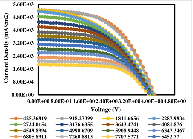
0.00E+00 8.00E-01 1.60E+00 2.40E+00 3.20E+00 4.00E+00 4.80E+00
Curre nt Densi ty ( m A/cm 2 ) Voltage (V)
[image:36.612.178.491.208.434.2]425.36819 918.27399 1811.6656 2287.9834 2724.0154 3176.6355 3643.4741 4081.876 4549.8994 4990.6709 5908.9448 6347.3467 6805.8911 7260.8813 7707.5771 5452.77
Figure 2-24 JV Curves of Thin FRP (Specimen 1).
Figure 2-25 JV Curves of Thin FRP (Specimen 3).
shown in Figures 2.24, and 2.25. From Figures 2.24, and 2.25, it can be seen the variation of
the J-V curves while the load is being applied. Specimen 1 in Figure 2.24 shows a uniform
degradation of J-V curves, because the MPP of the first specimen decreases linearly. The J-V
Curves decrease when the strain increases.
[image:36.612.176.495.457.693.2]0.00 0.20 0.40 0.60 0.80 1.00 1.20
0.00E+00 1.50E+03 3.00E+03 4.50E+03 6.00E+03 7.50E+03
No rm a li zed M a x Po w er Po in t, M PP Strain (με) Thin FRP # 1
[image:37.612.150.479.154.408.2]Thin FRP # 2 Thin FRP # 3 Thin FRP # 4 Thin FRP # 5
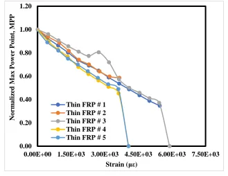
Figure 2-26 MPP vs. Strain of Thin FRP Specimens.
To study the effect of the J-V curves variation on the performance of the solar cell, the
relationship between MPP and strain of solar cells attached to thin FRP plate specimens is
plotted in Figure 2.26.
From Figure 2.26, it can be seen that the buckling effect becomes visible on the thin
FRP specimens when the specimens are being subjected to high strain. The overall trend is the
same for all specimens. There is almost a linear reduction in the power of the solar cell. The
MPP of the specimens 3, and 4 dropped to a value of zero because of the deficient connection
between the solar cell and the source meter used to extract the JV-curves and the solar cell
parameters. Specimen 1 has the largest strain value of 5400 με because the specimen was
exposed to excessive buckling as shown in figures 2.27 (b). During the test, different buckling
modes occurred at different strains as shown in Figure 2.27 (a), and (b). The specimens kept
0 200 400 600 800 1000 1200 1400 1600 1800 2000 2200 2400
0 0.2 0.4 0.6 0.8 1
Load
(
Ib)
[image:38.612.106.263.71.257.2]Displacement (in)
Figure 2-27 (a) Initial buckling mode. (b) Maximum buckling mode.
Figure 2-28 Load- displacement Curve of Neoprene Rubber Specimen 1 (Flat). 2.4.3 Neoprene Rubber
Rigid substrate as concrete used as supporting system was not beneficial in terms of
observing the degradation of the solar cell. Therefore, it is necessary to find a supporting
system satisfying these criteria. Neoprene Rubber meets these criteria. As a result, two
configuration of flat and curved solar cell attached to the Neoprene Rubber were investigated.
A STAEC machine used to induce compression load to the specimens as described in section
[image:38.612.350.508.72.260.2]0.00E+00 4.00E-04 8.00E-04 1.20E-03 1.60E-03 2.00E-03 2.40E-03
0.00E+00 1.20E+00 2.40E+00 3.60E+00 4.80E+00
Curre
nt
Densi
ty
,
J
sc
(m
A/cm
2
)
Voltage (V)
[image:39.612.159.477.479.694.2]0 0.0502524 0.1019232 0.1529559 0.2057994 0.2513403 0.300888 0.3524787 0.4030092 0.4511979 0.5004405 0.551151 0.600606 0.6500295 0.7005915 0.7572915 0.8017515 0.8509455 0.9003555
Figure 2-29 J-V characteristics curves of Neoprene Rubber (Flat Solar Cell) (Specimen 1). Figure 2.28 shows the load-displacement curve of the Neoprene Rubber. The load was
applied manually to control the required displacement, and have enough time to capture the
performance of the solar cell in both configurations (flat and curved solar cell). As it can be
seen from Figure 2.28, there are multiple steps shown in the curve. These steps were the
displacement values, which have been used in measuring the performance of the solar cell, and
when the load is not being applied.
The flat solar cell was attached directly to the Neoprene Rubber, while the curved solar
cell was attached to FRP substrate. The normal, FRP-confined, and FRP-wrapped concrete
specimens used as supporting systems, but the performance of the solar cell was not changed,
and just had rapid degradation when the failure exists. Therefore, it is necessary to find
supporting system that allows large deflection. As a result, The Neoprene Rubber could be
used as supporting systems as they have been used in civil engineering.
In order to investigate the performance of the solar cell attached to Neoprene Rubber.
The J-V characteristics curve was measured using a source meter and a lab view for both of
0.00E+00 4.00E-04 8.00E-04 1.20E-03 1.60E-03 2.00E-03 2.40E-03
0.00E+00 8.00E-01 1.60E+00 2.40E+00 3.20E+00 4.00E+00 4.80E+00
Curre nt Densi ty ( m A/cm 2 ) Voltage (V)
0 0.052083 0.100017 0.153198 0.200088
0.250443 0.30213 0.350604 0.401022 0.452628 0.503541 0.552528 0.603036 0.654606 0.702702 0.7533 0.802818 0.850581 0.9027
0.00 0.10 0.20 0.30 0.40 0.50 0.60 0.70 0.80 0.90 1.00 1.10 1.20 1.30
0 0.2 0.4 0.6 0.8 1
No rm a lized M P P Displacement (in)
[image:40.612.162.479.99.345.2]Sample 1 Flat Sample 2 Flat
Figure 2-30 J-V characteristics curves of Neoprene Rubber (Flat Solar Cells) (Specimen 2).
[image:40.612.164.480.408.622.2]Figure 2-32 Local Buckling of Flat Solar Cell (Specimen 2).
The relationship of MPP and displacement of the amorphous silicon solar cell attached
to Neoprene Rubber was obtained and plotted in Figure 2.31. The power in Watts obtained
from these two flat specimens were identical with an exception of the portions within a
displacement range of 0.1 in to 0.8 in. The power from the flat solar cell in specimen 2 is
reduced in this portion because of the local buckling located just above the center of the solar
cell. This local buckling reduces a portion of the area of the amorphous silicon solar cell as
shown in Figure 2.32.
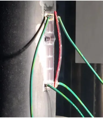
The second solar cell in figure 2.32 presents the curved amorphous silicon solar cell,
which is attached to the FRP substrate. It is supported at the both end of the solar cell. The
purpose of introducing the curvature mode is to expedite the process of buckling behavior.
The J-V curves were obtained for the second and third specimens, along with the relationship
between Maximum Power Point (MPP) vs. displacement as shown in Figures 2.33, 2.34 and
0.00E+00 4.00E-04 8.00E-04 1.20E-03 1.60E-03 2.00E-03
0.00E+00 1.20E+00 2.40E+00 3.60E+00 4.80E+00
Curre nt Densi ty , J sc (m A/cm Voltage (V)
0 0.052956 0.103185 0.25317 0.301725
0.352377 0.401517 0.453852 0.506574 0.552087 0.600246 0.650808 0.703881 0.750771 0.801054 0.854028 0.900792 0.950148 1.003239
0.00E+00 4.00E-04 8.00E-04 1.20E-03 1.60E-03 2.00E-03 2.40E-03 0.00E+008.00E-011.60E+002.40E+003.20E+004.00E+004.80E+00 Curre nt Densi ty ( m A/cm 2 ) Voltage (V)
[image:42.612.154.474.66.308.2]0 0.050688 0.103968 0.151839 0.200709 0.251811 0.300897 0.350235 0.40104 0.451494 0.600705 0.653688 0.703179 0.754533 0.80037 0.852975 0.901818
Figure 2-33 J-V characteristics curves of Neoprene Rubber (Curved Solar Cells) (Specimen 2).
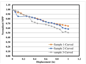
[image:42.612.148.478.350.603.2]0.00 0.10 0.20 0.30 0.40 0.50 0.60 0.70 0.80 0.90 1.00 1.10
0 0.2 0.4 0.6 0.8 1 1.2
No
rm
a
lized
M
P
P
Displacement (in)
[image:43.612.140.484.66.322.2]Sample 1-Curved Sample 2-Curved sample 3-Curved
Figure 2-35 MPP vs. Displacement of Curved amorphous Solar Cell Specimens.
Fill Factor is an important parameter that identifies whether the solar cell works
properly or not. The Fill Factor is a measurement of the squareness of the solar cell, and the
largest rectangular shape that fits inside the JV-curve. It can be noticed from Figure 2.33 and
2.34 that curved solar cells have lower values of Fill Factor (FF) compared to those of the flat
specimens as in Figures 2.29, and 2.30. The rectangular area decreases as the strain caused by
applied load increases. This effects the performance of the solar cell as shown in Figure 2.34.
The solar cell continues to decrease as the load is applied, and has almost a linear relationship
The efficiency of the amorphous silicon solar cell depends on multiple variables, such as short
circuit current, open circuit voltage, and fill factor (FF) of the solar cells. Various types of solar
cells have different efficiency. For instance, the maximum efficiency of the cadmium telluride
(CdTe) is 22.1%, while the amorphous silicon solar cell is between 4% to 14% (Jelle et al.,
2012). The short circuit current (Isc) is directly proportional to the light intensity. Therefore, as
the light intensity increases, the short circuit current (Isc)would increase and vice versa. The
open circuit voltage (Voc) is mainly affected by the high temperature as it increases. Therefore,
the open circuit voltage (Voc)is inversely proportional with the high temperature. The fill factor
(FF) is reduced when the amorphous silicon solar cell is subjected to high strain. It is noticed
in the previous results of the thin FRP and the rubber cylinders that the buckling behavior has
a significant impact on the amorphous silicon solar cells as their maximum power points
decreased in addition to the reduction in the efficiency of the amorphous silicon solar cells. In
this chapter, a numerical model was proposed that could calculate the reduction in the area of
the amorphous silicon solar cell at different stages of the applied loads, which is used to
determine the relative efficiency of the amorphous silicon solar cell . The buckling might occur
when the structural element is subjected to the axial load, such as columns. To derive the
numerical model, the function of the buckling shape has to be figured out. The curved
amorphous silicon solar cell is assumed to be simply supported. The proposed numerical model
used the buckling behavior of column, due to the similarity in the buckling shape. The
following equation (3) is the result from the free body diagram of the buckled column
where the P is the applied load, y is the transverse displacement, and M is the moment resulted
from the moment equilibrium. The relationship between the moment (M) and the transverse
displacement (y) for the elastic curve is given by the following equation (4):
EI (
dy2𝑑𝑥2
) = M
(4)Substituting the moment (M) from equation (4) into equation (3), and then divided both terms
by EI. This will result in the following equation (5):
𝑑2𝑦 𝑑𝑥2
+
𝑃
𝐸𝐼
𝑦 = 0
(5)The governing equation mentioned above is a second order homogenous ordinary differential
equation. The solution of the governing equation is given in equation (6).
𝑦(𝑥) = 𝐴 𝑠𝑖𝑛√𝑃
𝐸𝐼𝑥 + 𝐵 𝑐𝑜𝑠√ 𝑃
𝐸𝐼𝑥 (6)
The coefficients A and B can be determine based on the two boundary conditions y (0) = 0,
Eventually the shape function of the buckled shape is given in equation (8). It is important to
know that this equation is applicable to simply supported span.
𝑦(𝑥) = 𝐴 sin (𝑛𝜋𝑥
𝑙 ) (8)
where A is the maximum lateral displacement, n is the mode shape and is determined to be 1
when the mode shape is a half sine wave, and 𝑙 is the length of the solar cell. To determine the
length of the curved amorphous silicon solar cell, the equation of the arch length would be
applied as shown in equation (9).
𝑑(𝑠) = ∫ √1 + 𝑦𝑏 2(𝑥)′𝑑𝑥
𝑎 (9)
when the amorphous silicon solar cell buckles, the applied current makes an angle with the
surface of the solar cell. To have the current be applied perpendicular to the surface of the solar
cell, the current has to be multiply by cosѳ, where ѳ is the angle and calculated from the
derivation of the shape function given in equation (8), which was derived in equation (10).
𝑦
′(𝑥) =
𝜋 𝐶𝑜𝑠(𝜋𝑥
𝑙)
Figure 2-36 Area under Curved Solar Cell.
To obtain the area of the curved silicon solar cell before applying the load, the proposed
equation (11) can be used.
∫ 𝐶𝑜𝑠(𝑎𝑏 𝑦(𝑥)′) ∗ 𝑑(𝑠) 𝑑𝑥 (11)
where d(s) is the arch length given in equation (9), and 𝑦(𝑥)′ is given in equation (10),
𝑙
inequation (10) is equal to 2 in (Length of the flat solar cell).Then the equation has its final form
as shown in equation (12).
∫ 𝐶𝑜𝑠 (𝜋 ∗ cos ( 𝜋𝑥
𝑙 )
𝑙 )
𝑏
𝑎
∗ √1 +𝜋
2cos2(𝜋𝑥
𝑙 )
𝑙2 𝑑𝑥 (12)
The area of the flat silicon solar cell is 1 in2. The area of the curved silicon solar cell as
a function of the displacement was computed using equation (12). Then the result was graphed
cell during the test of the first specimen of thin (FRP). The remaining specimens are included
in the appendix. The maximum power points (MPP) in this case were calculated using equation
(1) mentioned in section 2.4.1. The area of the solar cell used in Equation (1) was based on the
area of the flat solar cell (1in2). Table 2.9 shows the calculation of the area of the curved solar,
and the corresponding relative efficiency.
Table 2-9 Calculations of Ac, and Relative Efficiency (Thin FRP Specimen # 1).
As it can be seen from tables 2.8, and 2.9, the buckling behavior of the silicon solar cell
has a significant impact on the relative efficiency of the amorphous silicon solar cell. The
relative efficiency continues to decrease due to the reduction in the area of the amorphous
silicon solar cell receiving the light as calculated in the column of the curved area. The initial
relative efficiency of the silicon solar cell is 1.0, which is corresponding to 100% energy
conversion before the starting the test, and drop down to 0.484, which is corresponding to
48.4% energy conversion at the end of the test. The maximum difference between the test data
Compression tests on solar cells attached to rigid (concrete) and flexible (thin FRP)
substrates were conducted. It was found that the performance of the solar cells attached to rigid
concrete substrate remained almost constant until the specimens failed, where a sudden drop
occurred. Degradation of the performance was observed for solar cells attached to flexible FRP
plate. It can be concluded that strain has negligible effect on solar cells under pure compression
because of its small deflection, but has a significant effect on solar cells under buckling because
of the change in the area receiving the sun light, which in turn causes the light intensity to be
decreased.
Compression test on two different configurations of solar cells attached to Neoprene
Rubber used as supporting system was also conducted. In case of flat solar cell, the
performance of the solar cells was almost constant with a minor reduction because of the local
buckling occurred above the mid-span of the solar cell, while for the curved solar cell, the
performance of solar cell has almost a linear trend in the first and second specimens. It is
concluded that in order to observe the reduction in the power of the solar cell, it is important
that the solar cell be attached to a supporting system that allows large deflection, and subjected
to a curvature shape during the installation of the solar cell to expedite the buckling behavior.
Relative efficiency is reduced due to the reduction in the area of the amorphous silicon
solar cell caused by the buckling of the amorphous silicon solar cell. The difference of the
relative efficiency of the amorphous silicon solar cell between the start and end of the test is
CHAPTER 3. PERFORMANCE OF SOLAR CELLS INTEGRATED WITH CONFINED FRP REINFORCED CONCRERTE UNDER FLEXTURAL TEST
3.1 MATERIAL PROPERTIES
3.1.1 Concrete Properties
The concrete used in this experiment was Portland Cement Concrete. The concrete used
to manufacture eight FRP-confined reinforced beams with a cross section area of 6 in x 6 in,
and a span length of 36 in. Six cylinders were prepared at the time of pouring the concrete in
order to evaluate the strength of the concrete at 7 and 28 days. The average compressive
strength and the standard deviation of the concrete cylinders are illustrated in Table 3.1.
Table 3-1 Average strength and standard deviation (Yossef 2017).
Date Tested Average strength, psi (MPa) Standard deviation, psi (MPa)
7 Days 3213 (22.15) 938 (6.46)
28 Days 5988 (41.29) 248 (1.7)
3.1.2 Steel Reinforcement
The Steel rebars used were ASTM A615 Grade 60 steel, with a yield strength of 60 ksi
(414 MPa). No. 4 steel rebars with a nominal diameter of 0.5 in (12.7 mm) were used as the
flexural reinforcement. They were cut to fit into the eight FRP-confined reinforced beams
specimens. The placement of steel rebars relies on the location of the tensile stress. In the case
when the solar cell that is attached to FRP is subjected to compression, two No.4 steel rebars
were placed in the tension region and the concrete side. In the other case when the solar cell is
subjected to tension, one No. 4 steel rebar was placed in the FRP side. The FRP is intended to
work as a shear reinforcement of the beam specimens based on (Brady and Marshall 1998),
placed at a distance of 1.5 in (concrete cover) from each edge of the concrete according to
(ACI 318-14, 2014). Figures 3.1, 3.2, and 3.3 show the placement of the steel reinforcement
according to the location of the tensile stress along with concrete cover.
Figure 3-1 Steel Reinforcement and concrete cover Figure 3-2 Steel Reinforcement at tension (FRP)
Figure 3-4 (a) Oil Spread on the Formwork. (b) Nylon ply Sheet and Solar Cell. 3.2 MATERIAL FABRICATIONS
3.2.1 FRP Fabrication
The FRP used in this experiment is chopped strand mat (CSM) with the properties
described in section 2.1.2. The formwork used to manufacture the beam specimens was the
typical modulus beam that has a cross section area of 6 in x 6 in with a span length of 36 in.
An oil was spread on the surface of formwork to facilitate the removal of the specimens after
being manufactured as shown in Figure 3.4(a). A nylon ply was placed on the formwork to
facilitate removal of the FRP, and to place the thin film silicon solar cell on the nylon ply at
the mid-span of the specimens as shown in Figure 3.4(b). To ensure that the solar cell will be
subjected to the same strain as the specimens, the solar cell was attached to FRP before the
fabrication process. This would make solar cell to be a part of the FRP material. The chopped
strand mat (CSM) was cut into the proper size and placed inside the formwork. The size of the
aggregate used was based on (Cho et al. 2010), who conducted an experiment to study the
effects of aggregate size and density on the shear and tensile bond characteristics of the coarse
sand between the FRP formwork and concrete. They concluded that the optimal aggregate size
was 4-7 mm (0.16-0.3 in), and the optimal aggregate distribution density was 4 kg/m2 (0.82
Figure 3-5 (a) Aluminium Clips and the Aggregates. (b) Poured Concrete.
fit inside the formwork. The process of manufacturing of the specimens was in three stages. In
the first stage, the 404-isophthalic resin was distributed evenly on only the bottom surface of
the specimen where the solar cell located. Then the aluminum roller was used to eliminate the
air bubble that might exist, ensure that the chopped strand mat (CSM) absorbs the resin, and
ensure that solar cell becomes an integrate part of the FRP. An aluminum clips was used to
hold both sides of the specimen from falling down as shown in Figure 3.5 (a). After applying
the roller on the resin, the aggregate was distributed above the bottom surface and then waited
until the aggregate was bonded to the FRP as shown in Figure 3.5(a).The same procedure was
applied to both sides of the specimens at different times. Once the specimens was
manufactured, steel reinforcements were placed and concrete was poured as shown in Figure
3.5 (b). A vibration machine was used to eliminate the voids and mix the concrete. The
specimens were taken off the formwork after they achieved the full strength as shown in Figure
3.6. The exceeded side of the FRP was removed (Figure 3.7) to have the same height as the
Figure 3-6 Final FRP Confined beam specimens Figure 3-7 Exceeded height at both FRP sides.
3.2.2 Strain Gauge Installation
Sixty-four strain gauges were placed to eight reinforced beam concrete with
FRP-confined. Eight strain gauges were attached to each specimen where four strain gauges were
attached to FRP surface, and the other four strain gauges were attached to the concrete surface.
The process of installing strain gauges, and type of strain gauges in each side of the specimen
was different because of the material properties. To install the strain gauges on the concrete
surface, a grinding machine was used to smooth the surface of the concrete where the strain
gauge located as shown in Figures 3.8 (a), and (b), respectively. The glue was used to fill the
voids in the concrete as shown in Figure 3.9. After the glue dried, the grinding machine with a
soft grinder was used again to remove the glue. A visual inspection was conducted to check
that the voids have been filled with glue. An acetone was applied to the location of the strain
gauges that was smoothening to remove the dust and clean the surface before installing the
strain gauges. The strain gauge with a gauge length of 60 mm (2.4 in) was attached on the
[image:55.612.85.276.99.267.2]Figure 3-8 (a) Grinding Machine. (b) smoothed surface of concrete
Figure 3-9 Placement of glue. Figure 3-10 Strain Gauge Configuration (60 mm). in the middle third of the third-point bending loading, and just outside of this region at both
directions at both cases when the solar cell is subjected to compression and tension as shown
[image:56.612.90.280.418.588.2]Figure 3-11 Optimal locations of strain gauges (Solar cell subjected to Compression).
Figure 3-12 Optimal locations of strain gauges (Solar cell subjected to Tension).
To install the strain gauges on the FRP surface, the surface preparation was achieved
in the following sequence. Interlux 202 Fiberglass Solvent Wash was used to clean the surface,
and then the surface was abraded with 40-grit sand paper. The surface was cleaned again with
the same Solvent, and then the surface was abraded with 230-grit sand paper. Then the surface
was cleaned 400-grit sand paper. The surface was cleaned with acetone as the final step. The
strain gauges with a gauge length of 5 mm (0.2 in) was used to attach on the FRP surface since
the FRP has small deflection as shown in Figure 3.13. The location of the strain gauges at both
cases where the solar cell is subjected to compression or tension were the same for the strain
gauges placed on the surface of the concrete as shown in Figures 3.14, and 3.15. Figures 3.16
(a) and (b) illustrate the test setup including the location of the deflection transducers numbered
Figure 3-13 Strain Gauges Placed on FRP Layer (5 mm gauge length).
Figure 3-14 Optimal locations of strain gauges (Solar cell subjected to Compression).
Figure 3-16 (a) Test Set-up of Solar cell under Compression (b) Test Set-up of Solar cell under Tension.
3.3 TESTING SETUP
3.3.1 Three Point Loading Flexural Testing
The reinforced concrete beam with FRP-confined specimens were tested under three-
points loading, according to ASTM standards (C78/C78M 2010). The purpose of this
experiment is to study the performance of the amorphous silicon solar cell under flexural
loading since the solar cell is installed on the building roofs, which is exposed to bending
moment. Therefore, it is important to investigate the performance of the silicon solar cells
under this type of load.
A frame holding two actuators was constructed. The two actuators have a load range
of 20 Kips for each actuator, which were connected to manual hydraulic jack to apply the load
on the solar cell under compression as shown in Figure 3.17 (a). The load from the actuator 2, 3
4 1
2, 3