Selection of Nodes on the Basis of Loading Probabilities

(1)

Selection of Nodes on the Basis of Loading

Probabilities

Nidhi Usrethe1, Deepak Paranjape 2

M. Tech Scholar, Dept. of CSE, Global Engineering College, Jabalpur, MP, India1 Assistant Professor, Dept. of CSE, Global Engineering College, Jabalpur, MP, India2

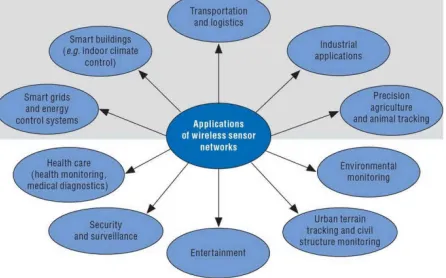
ABSTRACT: An emerging class of Wireless Sensor Network (WSN) applications involves the acquisition of large amounts of sensory data from battery powered, low computation and low memory wireless sensor nodes. The topology of the WSNs can vary from a simple star network to an advanced multi-hop wireless mesh network. The propagation technique between the hops of the network can be routing or flooding. In computer science and telecommunications, wireless sensor networks are an active research area with numerous workshops and conferences arranged each year to improve the performance of the network by using the Probability theory. The conclusion is that if balancing is achieved then all the nodes are always at equal energy level, so that there is no need to measure all the nodes. The measurement may be done by any of the nodes. All the nodes will be dead almost simultaneously. This analysis helps in deciding the better nodes. If balancing may not be achieved then we must select the node having lowest Loading Probability. This method of selection of nnooddee will be very useful for reducing the Traffic jam and risk of Failure the CH in LEACH Protocol.

KEYWORDS: CH, LEACH, WSN, routing, flooding, topology.

I. INTRODUCTION

(2)

II. RELATED WORK

A

Annuuppkkuummaarr MM BBoonnggaallee,, AAnnaannddSSwwaarruuppaannddSShhaasshhaannkkSShhiivvaammeett aall 22001177[[11]],, Design and improvement of vitality effective directing conventions for Wireless Sensor Network (WSN) is one of the dynamic research fields. Bunch based steering conventions have turned out to be vitality proficient and LEACH is one of most mainstream group based directing convention for WSN. In any case, LEACH experiences a few downsides, for example, plausibility of picking a low vitality hub as Cluster Head (CH) and non-uniform (unbalancing) dispersion of CHs, and so forth. In this paper EiP-LEACH (Energy affected Probability based LEACH) convention is proposed which is an upgraded adaptation of LEACH convention that is impacted by the vitality parameter for CH determination. EiP-LEACH helps in choosing the better CH hubs and in this manner contributes towards system life prolongation. EiPLEACH is contrasted and fundamental LEACH regarding number of alive hubs, normal vitality exhaustion, First Node Dead (FND) and Last Node Dead (LND) and found that EiP-LEACH is much better [1]. DDhhaarraammVViirr,,DDrr..SS..KK..AAggaarrwwaallaannddDDrr..SS..AA..IImmaamm

e

ettaall22001122[[55]] we saw that control sparing is an imperative advancement objective in remote sensor organize, the power devoured amid correspondence is more overwhelming than the power expended amid preparing on account of Limited stockpiling limit, Communication capacity, figuring capacity and the constrained battery are primary confinements in sensor systems. As the lifetime of the system is rely upon the battery life of the hubs, the plan of intensity effective directing conventions is must. By the perceptions we think about that the effect of intensity limitations on hubs in physical layer and application layer of the systems that DSR offers the best mix of intensity utilization and normal start to finish postpone execution. It has been seen that OLSR has preferred system lifetime over other. Future work, we can decrease the waste power utilization of the hubs by diminishing the quantity of directing control bundles and lessening the power devoured by hubs in an expansive system to build the existence time of system.

Arumugam eett aall 22001155[[11]], the creators proposed a vitality directing convention relies upon the compelling troupe ,

information and ideal bunch head choice. This convention drags out the lifetime of the system. Yet, regardless it experiences the postponement brought about by multifaceted activities. It generally picks the sensor hub that has higher leftover vitality without thought to some other factors, for example, the area of the sensor hub that might be situated far from BS. The motivation to work in this research area is the Dynamic Processing techniques which play a significant role in saving the time. In general algorithm however, choosing the best Node is not a trivial task and a bad choice will give a poor performance. The document delivery speed between a server and a client (Node) depends on the server load, the file retrieving speed at the server, the available bandwidth between the server and the client, and the client load. In this work, we investigate two problems: one deal with finding the Maximum Loading Probabilities. We call it MaxLP problem. The other deals with finding the best group of k Nodes having Minimum Loading Probabilities. We called it MinLP problem. It is assumed that the network topology, the path bandwidth and server performance are known and static. The main objective of the exploration work talked about in this theory is to investigate the execution of novel key pre-appropriation plans for expanding the versatility of the system. The second objective is to investigate vitality productivity bunching approaches which builds the vitality effectiveness of the system. The sensor hubs are utilized to gather and report information to the sensor hub, known as a sink hub. By utilizing a bunching system progressive directing convention enormously limit the vitality devoured in gathering and appropriating the information.

III. CHALLENGES OF WSN

Energy is the scarcest resource of WSN nodes, and it determines the lifetime of WSNs. WSNs are meant to be deployed in large numbers in various environments, including remote and hostile regions, where ad hoc communications are a key component. For this reason, algorithms and protocols need to address the following issues:

 Lifetime maximization

 Robustness and fault tolerance

(3)

IV. PROPOSED METHODOLOGY

In our research, the ultimate aim is to give an idea for selecting the Node in a generic WSN application with essential and definable Load (Throughput) constituents and the relationship among these constituents so that one can explore strategies for minimizing the overall Congestion and traffic of the entire application. Presently the Wireless Sensor Network in India uses the high resolution Image cameras in the node stations, which are able to capture a picture nicely and then transmit the image towards the central office or Server base station. The data gathered from wireless sensor networks is usually saved a central base station (Server). If a centralized architecture is used in a sensor network and the central node fails, then the entire network will collapse, however the reliability of the sensor network can be increased by using distributed control architecture. This architecture has a drawback that there is a lot of energy consumption and congestion during the propagation of data. The most demanding requirement of wireless sensor hierarchy is to increase the lifetime and decrease the Transmission Delay in the architecture as all the Nodes are prepared with critical battery power.

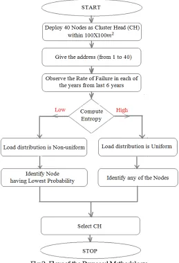
Fig 2: Flow of the Proposed Methodology

(4)

described in average Load per individual node, called Entropy. Let M= Total number of nodes

=− ∑ .log Load/ Node

Then entropy is maximum; if all the nodes have equal load.

For example if we are tossing a coin, then there may be 2 outcomes Head & Tail; it means P=1/2 and Q=1/2. Now entropy for Binary Numbers [H & T] is-

=−[ .log + .log ]

=−log [2].

= 1 Outcome / Toss

This shows that Average or Entropy is maximum if all the probabilities are equal. It means to achieve the load balancing, routing should be such that all the nodes have handled equal traffic load. This is the condition of balancing the Load. If balancing is used then all the Nodes share equal amount of Load. Therefore, the Failure Probabilities of all the Nodes are almost equal. Now the Leach Protocol will be very secure because it can select any of the Nodes as Cluster Head. By this there is no problem of die the Cluster Head before completing the communication. In our simulation, 50 sensors are deployed in 100X100 area that generates data from environment events at random times and places within the area. Sensing applications could equally environment temperature, pollution, or others. We considered the prevalent parameters of energy consumption of process, memory and radio units as constant in the individual constituent of all sensors. Also the duration of the experiments was assumed as constant 60 seconds. Monitoring neighbors and providing a secure communication with neighbors at the local level. In addition, the local constituent may include overhearing, idle listening and collision, if they occur. The global constituent is concerned with maintenance of the whole network, selection of a suitable topology and an energy efficient routing strategy based on the application’s objective. This may include energy wastage from packet retransmissions due to congestion and packet errors. The global constituent is defined as a function of energy consumption (EC) for topology management, packet routing, packet loss, and protocol overheads. The sink constituent includes the roles of manager, controller or leaders in WSNs. The sink tasks include directing, balancing, and minimizing EC of the whole network and the collection of generated data by the network’s nodes.

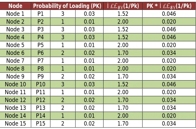
Table 1: Entropy Calculation for 50 Nodes Loading Probabilities

Node Probability of Loading (PK) (1/Pk) PK * (1/Pk)

Node 1 P1 3 0.03 1.52 0.046

Node 2 P2 1 0.01 2.00 0.020

Node 3 P3 3 0.03 1.52 0.046

Node 4 P4 3 0.03 1.52 0.046

Node 5 P5 1 0.01 2.00 0.020

Node 6 P6 2 0.02 1.70 0.034

Node 7 P7 1 0.01 2.00 0.020

Node 8 P8 1 0.01 2.00 0.020

Node 9 P9 2 0.02 1.70 0.034

Node 10 P10 3 0.03 1.52 0.046

Node 11 P11 1 0.01 2.00 0.020

Node 12 P12 2 0.02 1.70 0.034

Node 13 P13 2 0.02 1.70 0.034

Node 14 P14 1 0.01 2.00 0.020

(5)

Node 16 P16 3 0.03 1.52 0.046

Node 17 P17 2 0.02 1.70 0.034

Node 18 P18 4 0.04 1.40 0.056

Node 19 P19 1 0.01 2.00 0.020

Node 20 P20 2 0.02 1.70 0.034

Node 21 P21 3 0.03 1.52 0.046

Node 22 P22 2 0.02 1.70 0.034

Node 23 P23 1 0.01 2.00 0.020

Node 24 P24 2 0.02 1.70 0.034

Node 25 P25 1 0.01 2.00 0.020

Node 26 P26 1 0.01 2.00 0.020

Node 27 P27 3 0.03 1.52 0.046

Node 28 P28 5 0.05 1.30 0.065

Node 29 P29 2 0.02 1.70 0.034

Node 30 P30 2 0.02 1.70 0.034

Node 31 P31 1 0.01 2.00 0.020

Node 32 P32 2 0.02 1.70 0.034

Node 33 P33 5 0.05 1.30 0.065

Node 34 P34 3 0.03 1.52 0.046

Node 35 P35 1 0.01 2.00 0.020

Node 36 P36 1 0.01 2.00 0.020

Node 37 P37 6 0.06 1.22 0.073

Node 38 P38 4 0.04 1.40 0.056

Node 39 P39 1 0.01 2.00 0.020

Node 40 P40 2 0.02 1.70 0.034

Node 41 P11 1 0.01 2.00 0.020

Node 42 P12 1 0.01 2.00 0.020

Node 43 P13 1 0.01 2.00 0.020

Node 44 P14 1 0.01 2.00 0.020

Node 45 P15 1 0.01 2.00 0.020

Node 46 P16 1 0.01 2.00 0.020

Node 47 P17 1 0.01 2.00 0.020

Node 48 P18 3 0.03 1.52 0.046

Node 49 P19 1 0.01 2.00 0.020

Node 50 P20 1 0.01 2.00 0.020

TOTAL 100 1 H (X) = 1.62816

The condition of applying Probability theory is that the summation of all the Probabilities must be equal to 1. Here summation is 100. Now, divide each of the Probability by 100, and then the summation of all the Probabilities will be equal to 1. Let, calculate the Entropy.

Let Total number of Nodes=50

= 1.62816 Load/ Node

(6)

Probability is 0.025.

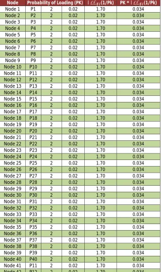
Table 2: Entropy Calculation for 50 Nodes with equal Loading Probabilities

Node Probability of Loading (PK) (1/Pk) PK * (1/Pk)

Node 1 P1 2 0.02 1.70 0.034

Node 2 P2 2 0.02 1.70 0.034

Node 3 P3 2 0.02 1.70 0.034

Node 4 P4 2 0.02 1.70 0.034

Node 5 P5 2 0.02 1.70 0.034

Node 6 P6 2 0.02 1.70 0.034

Node 7 P7 2 0.02 1.70 0.034

Node 8 P8 2 0.02 1.70 0.034

Node 9 P9 2 0.02 1.70 0.034

Node 10 P10 2 0.02 1.70 0.034

Node 11 P11 2 0.02 1.70 0.034

Node 12 P12 2 0.02 1.70 0.034

Node 13 P13 2 0.02 1.70 0.034

Node 14 P14 2 0.02 1.70 0.034

Node 15 P15 2 0.02 1.70 0.034

Node 16 P16 2 0.02 1.70 0.034

Node 17 P17 2 0.02 1.70 0.034

Node 18 P18 2 0.02 1.70 0.034

Node 19 P19 2 0.02 1.70 0.034

Node 20 P20 2 0.02 1.70 0.034

Node 21 P21 2 0.02 1.70 0.034

Node 22 P22 2 0.02 1.70 0.034

Node 23 P23 2 0.02 1.70 0.034

Node 24 P24 2 0.02 1.70 0.034

Node 25 P25 2 0.02 1.70 0.034

Node 26 P26 2 0.02 1.70 0.034

Node 27 P27 2 0.02 1.70 0.034

Node 28 P28 2 0.02 1.70 0.034

Node 29 P29 2 0.02 1.70 0.034

Node 30 P30 2 0.02 1.70 0.034

Node 31 P31 2 0.02 1.70 0.034

Node 32 P32 2 0.02 1.70 0.034

Node 33 P33 2 0.02 1.70 0.034

Node 34 P34 2 0.02 1.70 0.034

Node 35 P35 2 0.02 1.70 0.034

Node 36 P36 2 0.02 1.70 0.034

Node 37 P37 2 0.02 1.70 0.034

Node 38 P38 2 0.02 1.70 0.034

Node 39 P39 2 0.02 1.70 0.034

Node 40 P40 2 0.02 1.70 0.034

Node 41 P11 2 0.02 1.70 0.034

(7)

Node 43 P13 2 0.02 1.70 0.034

Node 44 P14 2 0.02 1.70 0.034

Node 45 P15 2 0.02 1.70 0.034

Node 46 P16 2 0.02 1.70 0.034

Node 47 P17 2 0.02 1.70 0.034

Node 48 P18 2 0.02 1.70 0.034

Node 49 P19 2 0.02 1.70 0.034

Node 50 P20 2 0.02 1.70 0.034

TOTAL 100 1 H (X) = 1.69897

= 1.69897 Load/ Node

Fig 3: MATLAB Program for Nodes Deployment and Probability Calculation in WSN

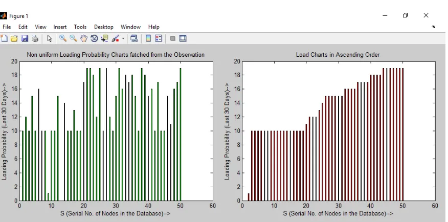
V. EXPERIMENTAL RESULTS AND CONCLUSION

(8)

Fig 4: Load Chart of Observed Data in WSN using MATLAB

REFERENCES

[1] Aliouat, Z, Harous, S., “An efficient clustering protocol increasing wireless sensor networks life time”, International Conference on Innovations in Information Technology (IIT), pp. 194 – 199, 2012.

[2] Baghyalakshmi, D., Ebenezer J., SatyaMurty, S.A.V., “Low latency and energy efficient routing protocols for wireless sensor networks”, International Conference on Wireless Communication and Sensor Computing, ICWCSC, pp. 1-6, 2010

[3] Johnson, M., Healy, M., van de Ven, P., Hayes, M.J., Nelson, J., Newe, T., Lewis, E., “ A comparative review of wireless sensor network mote technologies”, Sensors, IEEE, pp. 1439-1442, 2009.

[4] Wan Norsyafizan W,Muhamad,Nani Fadzlina Naim, “Maximizing Network Lifetime with Efficient Routing Protocol for Wireless Sensor Networks” Fifth International Conference on MEMS.2009,IEEE.

[5] Osawa, T.; Inagaki, T.; Ishihara, S., “Implementation of Hierarchical GAF”, 5th International Conference on Networked Sensing Systems, 2008. INSS, pp. 247, 2008.

[6] Ashish Gupta IT, Dev Bhoomi Inst. of Technology Bhupender Singh & Rautela Binay Kumar CSE, Graphic Era University, “Power Management in Wireless Sensor Networks”, International Journal of Advanced Research in Computer Science and Software Engineering, Volume 4, Issue 4, April 2014 ISSN: 2277-128X.

[7] Pratik R. chavda, Prof Paresh kotak, “Comparison LEACH and HEED Cluster Based protocol for Wireless Senser Network”, IOSR Journal of Computer Engineering (IOSRJCE) Volume 7, Issue 3 (Nov. - Dec. 2012), ISSN: 2278-0661.

[8] Jamal N. Al-Karaki, Ahmed E. Kamal, “Routing Techniques in Wireless Sensor Networks: A Survey”, Dept of Electrical & Computer Engineering, IEEE wireless communications, vol. 11, Dec 2004.

[9] Lan F. Akyildiz,Georgia Institute of Technology, USA and Mehmet Can Vuran, University of Nebraska-Lincoln, USA,“Wireless Sensor Network”, first published 2010, John Wiley & Sons Ltd.