Article
Novel
S
emi-parametric
A
lgorithm
for
I
nterference-immune
T
unable
A
bsorption
S
pectroscopy
G
as
S
ensing
Umberto Michelucci1,‡, Francesca Venturini2,‡*
1 udata.science,Dübendorf8600,Switzerland; [email protected]
2 InstituteofAppliedMathematicsandPhysics,ZurichUniversityofAppliedSciences,Winterthur8401,
Switzerland; [email protected]
* Correspondence: [email protected]
‡ These authors contributed equally to this work.
Abstract:One of the most common limits to gas sensor performance is the presence of unwanted 1
interference fringes or etalons arising, for example, from multiple reflections between surfaces in 2
the optical path. Additionally, since the amplitude and the frequency of these interference depend 3
on the distance and alignment of the optical elements, they are affected by temperature changes 4
and mechanical disturbances, giving rise to a drift of the signal. In this work, we present a novel 5
semi-parametric algorithm which allows the extraction of a signal, like the spectroscopic absorption 6
line of a gas molecule, from a background containing arbitrary disturbances, without having to 7
make any assumption on the functional form of these disturbances. The algorithm is applied first to 8
simulated data and then to oxygen absorption measurements in presence of strong fringes.To the 9
best of the authors’ knowledge, the algorithm enables an unprecedented accuracy particularly if the 10
fringes have a free spectral range and amplitude comparable to those of the signal to be detected. 11
The described method presents the advantage of being based purely on post processing, and to be 12
of extremely straightforward implementation if the functional form of the Fourier transform of the 13
signal is known. Therefore it has the potential to enable interference-immune absorption spectroscopy. 14
Finally, its relevance goes beyond absorption spectroscopy for gas sensing since it can be applied to 15
any kind of spectroscopic data. 16
Keywords: interference; interference cancellation; noise reduction; digital filtering; spectroscopy; 17
sensors. 18
1. Introduction
19
Due to the enormous progress in availability and performance of laser light sources and 20
electro-optical components, tunable diode laser absorption spectroscopy (TDLAS) has entered various 21
disciplines both in research and industrial applications. Being a high-sensitivity, selective, fast, 22
non-destructive and in-situ method, TDLAS is currently more and more used for quantitative 23
assessments of gas concentration in several fields. These include, to mention only few, atmospheric 24
environmental monitoring [1–6], medical diagnostics [7–9] chemical analysis [10] and industrial process 25
control [11–13]. The increasing number of applications has pushed the requirements on this method 26
both in terms of sensitivity and in terms of stability. On the other hand, for practical and commercial 27
applications there is a growing interest in compact, simple in design and cost-effective sensitive 28
sensors, which do not require special optical components but guarantee the sensitivity achievable with 29
a complex laboratory equipment. 30
One of the most common limits to the sensor performance is the presence of unwanted interference 31
fringes called etalons [14]. These interferences may arise due to multiple reflections from reflecting 32
or scattering surfaces in the system, like mirrors, lenses, optical fiber end faces, laser-head windows 33
or dust particles in the gas [14]. Even diffusive surfaces, as for example due to dust deposited on 34
the windows, can give rise to fringes over time [15]. Particularly fringes which have a free spectral 35
range (FSR) of the order of the width of the absorption lines contribute to significant errors in the 36
determination of the line features and require special strategies [16]. Additionally, since the amplitude 37
and the frequency of these interferences depend on the distance and alignment of the optical elements, 38
they are affected by temperature changes and by mechanical disturbances, giving rise for example to a 39
drift of the output signal, thus worsening the long-term performance of the system [17]. 40
The simplest strategy to reduce the effects of interference fringes consists in using anti-reflection 41
coating and wedging or angling of the optical surfaces. Other approaches include, to mention only few, 42
to dither one of the surface creating the interference and integrating the signal so to average out its 43
influence [18,19], the selection of a particular modulation frequency [20] or modulation scheme [21,22], 44
to specifically choose the distance between the interfering surfaces [23] and post-processing filtering 45
[24]. A comprehensive review on signal enhancement and noise reduction techniques can be found 46
in [25]. Although all these approaches have been successfully implemented in the past years, they 47
nonetheless have limitations in the practical implementation depending on the application-specific 48
conditions. For example, it may not always be possible to dither one surface, and the application of a 49
specific detection scheme may limit the flexibility of the measurement. 50
In this work a new and widely usable approach is presented, which relies only on post processing 51
of the data. Therefore it requires no modification to the apparatus setup or hardware, and can be 52
easily adapted to different experimental configurations. The new presented algorithm allows the 53
extraction of a signal, as the absorption lines of a gas molecule, from a background containing arbitrary 54
disturbances without having to make any assumption on the characteristic of these disturbances in 55
terms of functional form. Therefore, it has the potential to improve the sensitivity and the stability of 56
TDLAS. Furthermore, this algorithm, which is particularly easy in the implementation if the Fourier 57
transform of the signal can be written in closed form, is very general and can be applied to any kind 58
of spectroscopic data. The paper is organized as follows: section2describes the fundamentals of the 59
method and of the algorithm; section3demonstrates its application to simulated signals; section4 60
shows the results for a case of direct absorption spectroscopy for oxygen gas sensing. 61
2. Description of the algorithm
62
The algorithm described in this work has the ability to identify a spectroscopic feature from an arbitrary background which needs not to be modeled. The total signal detected in an experiment, here referred to as "total signal"Itot(x), is modeled as a sum of two contributions: one spectroscopic
feature, like an absorption line, here referred to as "signal"I(x)and a background here referred to as "background"B(x)
Itot(x) =I(x) +B(x) (1)
In the case of direct absorption spectroscopy, I(x) is the absorbance and Itot(x)is the distorted
63
absorbance due toB(x). As mentioned above, the method shines if the backgroundB(x) cannot 64
be modeled by a known analytical expression. In facts, ifB(x)is not known, is not possible to perform 65
a non-linear fit ofItot(x)and extract the signalI(x)without making assumptions on the functional
66
form ofB(x). On the other hand, if the functional form is known but very complex, the algorithm may 67
be advantageous because the inclusion of the background in the non-linear fit may not be possible. 68
Another significant advantage of the proposed algorithm is that the extraction works equally well 69
2.1. Steps of the algorithm: general description 71
Before describing the steps of the algorithm, the nomenclature and hypothesis for its applicability are introduced. The algorithm is based on the main hypothesis that the Fourier transform of the backgroundB(x)is significantly different than zero only for values ofksmaller than a certain cut-off k0
F(Itot)(k) =
(
F(I)(k) +F(B)(k)fork<k0 F(I)(k) +efork>k0
(2)
whereF(·)denotes the continuous Fourier transform (CFT),k0a cut-off frequency andecontains 72
the contribution ofF(B)(k)fork>k0, which is assumed to be negligible. One central aspect is the 73
determination of a reasonable estimate for this cut-off frequency, as described in the section "Determine 74
the cut-off frequency". 75
Note that this formulation applies to continuous functions. Since in practice there will always be only a discrete set of points, it is necessary to approximate the CFT in equation (2) by a modified discrete Fourier transform (DFT)
Di(Itot) =
(
Di(I) +Di(B)fori<i0 Di(I) +efori>i0
(3)
where Di(·) denotes the modified DFT defined in Appendix Aequation A7, i0 the cut-off point
76
corresponding to the cut-off frequencyk0, andecontains the contribution ofDi(B)fori>i0, which is 77
assumed to be negligible. 78
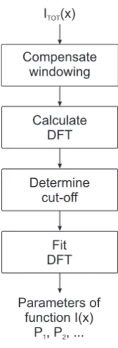
The schematic flow diagram of the algorithm is shown in Fig.1to give the reader a high-level 79
understanding of the idea behind it. The single steps are described in detail below.
ITOT(x)
Compensate windowing
Calculate DFT
Determine cut-off
Fit DFT
Parameters of function I(x)
P , P , ...1 2
Figure 1.Schematic flow diagram of the steps of the algorithm to extract a signalI(x)from a total signalItot(x).
80
Compensate windowing
81
In all real experiments the data always cover a limited range in thexdirection. For example, the 82
equivalent to applying a rectangular window (RW) before calculating the Fourier transform. This is a 84
problem that, if not addressed, will limit the precision that can be achieve with the described algorithm. 85
In facts, the RW results into makingein equation2not negligible anymore, and thus leads to an error 86
in the fitting procedure of|F(I(x))(k)|. This is due to the fact that the DFT of a RW has an amplitude 87
envelope which is proportional to 1/k, and so it does not goes to zero fast enough [26]. 88
To reduce the effect of windowing considerably the proposed algorithm applies a more 89
intelligent window. The not so often used Tukey window [27,28] has remarkable properties that 90
help tremendously in reducingedramatically. The Tukey window, indicated withT(x), is a perfectly 91
flat (constant) symmetric function in the middle that then decrease rapidly to zero on the sides. 92
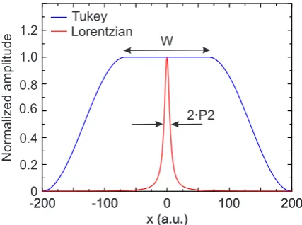
The width of the constant part of the Tukey function has to be chosen intelligently. Fig.2shows a Lorentzian function with a half width at half maximum (HWHM) indicated asP2and Tukey function with a width indicated asW, both functions normalized to 1 for clarity. As it is easy to understand from Fig. 2, ifWis significantly bigger thanP2thenT(x)I(x)can be approximated withI(x). Therefore, defining ˜Itot(x) =T(x)Itot(x), it follows
˜
Itot(x) =T(x)I(x) +T(x)B(x) (4)
This is the function of which the DFT has to be calculated, instead of simply usingItot(x). Equation4
can then be approximated under the assumption ofWbeing significantly bigger thanP2as ˜
Itot(x) =I(x) +T(x)B(x) (5)
˜
Itot(x)is thus the sum of the signal ofI(x)and a background which is the product of the original
93
backgroundB(x)andT(x). The modified backgroundT(x)B(x)has a Fourier transform that goes 94
to zero much more rapidly ([27,28]) and that means thateis much smaller if one considers ˜Itot(x)
95
instead ofItot(x). In other words, while using ˜Itot(x),ewill contain the contribution ofDi(T·B)that
96
is considerably smaller thanDi(B)multiplied by a RW.
97
Analyzing the deviation between the output of the algorithm and the input signalI(x)with 98
simulated data was performed, it was established that the algorithm works well if the width of the 99
Tukey window isW &20P2. In this workW = 20P2was used for both the simulated and for the 100
experimental data. The case withW=20P2is shown schematically in Fig.2. 101
Normalized amplitude
0 0.4 0.8 1.0
0.2 0.6 1.2
2 P2ā
W Tukey
Lorentzian
0 200
-200
x (a.u.)
-100 0 100 200
-200
x (a.u.)
-100 100
Figure 2.Schematic representation on how to choose the width of the Tukey windowWcompared to the Lorentzian HWHMP2. Here isW=20P2.
Calculate the DFT
102
The step after compensating for the windowing is the calculation of the DFT. To be able to extract 103
modified DFT as described in AppendixA. For all the data shown in this paper the DFT was calculated 105
using the formula (A7). 106
Determine cut-off
107
As shown in Fig. 1, the next step is to determine the optimal cut-off pointi0which plays an 108
important role and needs to be chosen carefully. The approach proposed in this work is to choosei0so 109
to maximize the coefficient of determinationR2obtained by fitting the DTF fori>i0. An example of 110
the implementation is described in the following algorithm written in pseudo code, whereNindicates 111
the number of points of the dataset (i.e. the finite number of experimantsl points),Dthe DFT of the 112
signal ˜Itot(x),Rsquaredthe coefficient of determinationR2calculated from the fit routines, andRlimit
113
the value which should be reached forR2. This limiting value can be helpful since beyond a certain 114
value, even if R2 continues to increase when increasingi0, the quality of the fit will not improve 115
significantly and it is not necessary to exclude more points from the DFT for the fit. 116
pointtoremove = 0 117
Rsqmin = 0 118
for i = 0 to N 119
remove i points from the data set 120
fit the remaining points of D and save the fit parameter Rsquared 121
if (i = 0) then pointtoremove = 0 122
else if (Rsquared > Rsqmin) then pointtoremove = i and Rsqmin = Rsquared 123
if (Rsqmin > Rlimit) then break loop 124
end of for loop 125
At the end of this loop in the above mentioned pseudo-codei0is determined and saved in the variable 126
pointtoremove.Rsquaredcan be chosen depending on the application. For the curves shown in this 127
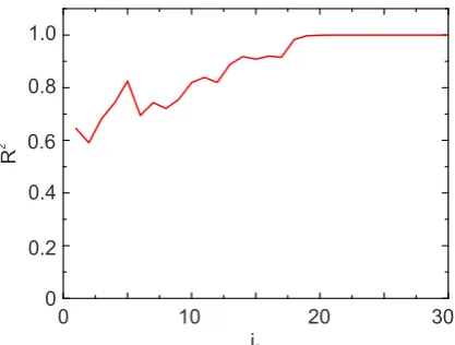
paper the loop was stopped forRlimit=0.99999. An example of the evolution ofR2with increasing 128
i0is shown in Fig.3. The data refer to the third scenario described later in section3. Abovei0=30,R2 129
still continue to slightly increase but the statistical goodness of the fit does not improve further. 130
R
2
0 0.4 0.8 1.0
0.2 0.6
20 30
0
i0 10
Figure 3. Evolution ofR2with increasing value of the cut-offi0. The data correspond to the third scenario described in section3.
Fit of DFT
131
The final step of the algorithm is to perform a non-linear fit of the DFT fori > i0. Since the 132
functional form of the DFT is known this is a standard procedure which can be performed, for example, 133
with least-square-fit routines and will not be discussed here. Since the functional form of|F(I(x))(k)| 134
2.2. Algorithm applied to a Lorentzian line shape 136
In this section the implementation of the algorithm to a Lorentzian function signalI(x)is described 137
as an example. This functional form was chosen because describes the absorption lines of many gas 138
molecules, as for example oxygen under atmospheric conditions. In other conditions, like at higher 139
temperatures or lower pressures, the Gaussian contribution due to Doppler broadening cannot be 140
neglected and a Voigt profile is a better description. 141
The Lorentzian function can be written as
I(x) = P1P2 π(x2+P2
2)
(6)
withP1,P2>0. In this formP1andP2represent the area and the HWHM of the line. WritingI(x)in this form is particularly advantageous since in direct absorption spectroscopy the gas concentration can be determined directly from the area under the line, thus is given directly byP1. In this formulation |F(I(x))(k)|is then a simple exponential
F(I(x))(k) =P1e−P2|k| (7)
So, once the parametersP1andP2are determined from the fit of the DFT,I(x)is known. 142
3. Application to simulated data
143
The novel algorithm was first applied to artificially simulated data to demonstrate its functioning 144
and its performance. Since the signal to be extracted I(x)is known, it is possible to estimate the 145
accuracy and robustness of the algorithm in presence of backgrounds with different characteristics. In 146
particular, three scenarios with different types of periodic disturbances were simulated. The signal to 147
be extractedI(x)is for all three cases the same Lorentzian function written in the form of Eq.6with 148
P1=5πandP2=5. All three scenarios were chosen to reflect real cases which are typical of TDLAS. 149
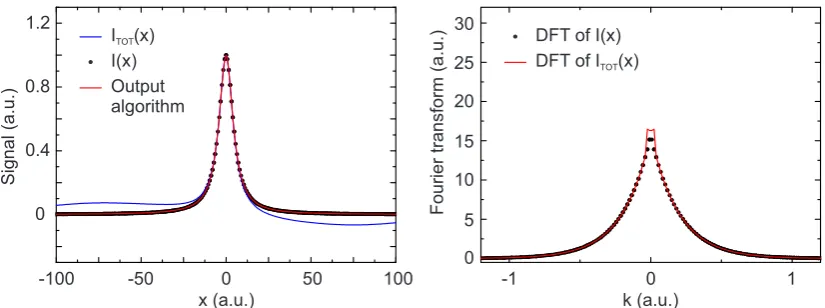
The first scenario is chosen to represent the experimental situation when the background has a periodic disturbance with a FSR comparable to the width of the line to be detected. This type of background is particularly problematic because it strongly affects the determination of the line shape. Furthermore, it cannot be removed by introducing a small jitter on the laser diode laser current and averaged out [29] or be filtered out with standard post-processing methods, without introducing a significant distortion to the line shape. This background taken here is a simple a cosine function
B(x) =0.07 cos(0.1x+1) (8)
The total signalItot(x)in this case, together with the expected signalI(x)are shown Fig.4on the left.
150
Also shown in the figure on the left is the result obtained by applying the described algorithm. Despite 151
the problematic background, the output of the algorithm is practically identical toI(x). The percent 152
deviation of the two parametersP1andP2describing the Lorentzian obtained with the algorithm from 153
the initial value used to generateI(x)is only of 0.27% forP1and 0.23% forP2. 154
To better illustrate the contribution of the background, the DFT of the Lorentzian and the DFT 155
of the total signal signal are also shown in Fig. 4on the right. The two peaks visible in the figure 156
represent the contribution of the background. With the pseudo-code algorithm described in section2.1 157
the cut-off wasi0=13. 158
DFT of I(x) DFT of ITOT(x)
0 1
-1
k (a.u.)
Fourier transform (a.u.)
0 5 10 15 20 25 30
Signal (a.u.)
0 0.4 0.8 1.2
0 100
-100
x (a.u.)
-50 50
ITOT(x)
I(x) Output algorithm
Figure 4. First scenario: disturbance with a FSR comparable to the line width. Left: Simulated experimental total signalItot(x)(blue line), Lorentzian line shape signalI(x)(black dots) and extracted
signal obtained with the algorithm (red line). Right: DFT of the total signal|F(Itot(x))(k)|(red line)
and DFT of the Lorentzian signal|F(I(x))(k)|(black points).
dimension, like the laser-chip output face and the glass window of the laser packaging. The chosen functional form to simulate this scenario is the following
B(x) =0.07 cos(0.02x+1.6) (9)
The result of the algorithm for this scenario are shown in Fig.5: on the left are plotted the total 159
signalItot(x), the expected signalI(x)and the result obtained by applying the algorithm. In Fig.5on
160
the right are shown the DFT of the Lorentzian and the DFT of the total signal signal. The two peaks 161
due to the contribution of the background are now very close to zero, which makes the extraction 162
particularly unproblematic. With the pseudo-code algorithm described in section2.1the cut-off was 163
i0=7. 164
Fourier transform (a.u.)
0 5 10 15 20 25 30
0 1
-1
0 100
-100
x (a.u.)
-50 50
Signal (a.u.)
0 0.4 0.8 1.2
DFT of I(x) DFT of ITOT(x) ITOT(x)
I(x) Output algorithm
k (a.u.)
Figure 5. Second scenario: weak disturbance with a FSR as large as the measuring window. Left: Simulated experimental total signalItot(x)(blue line), Lorentzian line shape signalI(x)(black dots)
and extracted signal obtained with the algorithm (red line). Right: DFT of the total signal|F(Itot(x))(k)|
(red line) and DFT of the Lorentzian signal|F(I(x))(k)|(black points).
Also in this case it is clear from the figure that the algorithm extracts exceedingly well the signal. 165
The percent deviation of the two parameters describing the Lorentzian obtained with the algorithm is 166
only of 0.28% forP1and 0.25% forP2. 167
interferences are, the algorithm can extract signalI(x)very well. Also, this scenario illustrate the case when the functional form of the background is too complex to be included in a non-linear fit ofItot(x).
The background is thus written as
B(x) = 100
∑
i=1
Aicos(wix+φi) (10)
wherewiare chosen randomly from a normal distribution with average equal to zero and a standard
168
deviation of 0.1,φifrom a normal distribution with average equal to zero and a standard deviation of
169
0.2, andAifrom a normal distribution with average equal to zero and a standard deviation of 0.03.
170
In Fig. 6on the left are shown the total signal Itot(x), the expected signalI(x)and the result
171
obtained by applying the described algorithm. Despite the very complicated background the extraction 172
of the signalI(x)by the algorithm works very well. In Fig.6on the right the DFT of the Lorentzian 173
and the DFT of the total signal signal are also shown. Due to the high number of cosine functions in 174
the background the DFT has a much structured shape. With the pseudo-code algorithm described in 175
section2.1the cut-off wasi0=30 (see also Fig.3). 176
Fourier transform (a.u.)
0
0 5
10 15 20 25 30
1 -1
0 100
-100
x (a.u.)
-50 50
Signal (a.u.)
0 0.4 0.8 1.2
DFT of I(x) DFT of ITOT(x) ITOT(x)
I(x) Output algorithm
k (a.u.)
Figure 6. Third scenario: strong multiple disturbances. Left: Simulated experimental total signal Itot(x)(blue line), Lorentzian line shape signalI(x)(black dots) and extracted signal obtained with the
algorithm (red line). Right: DFT of the total signal|F(Itot(x))(k)|(red line) and DFT of the Lorentzian
signal|F(I(x))(k)|(black points).
The percent deviation of the two parameters describing the Lorentzian obtained with the algorithm 177
for this scenario is only of 0.012% forP1 and 0.14% for P2. The deviation of both parameters is 178
particularly low in this case. To better estimate the error and the standard deviation on the parameters 179
the method was applied to 500 functions created with the random sum of 100 cosines described above. 180
Then the error was evaluated and its distribution studied. As a resultP1has a mean value of the 181
absolute value of the percentual error of 0.12% with a standard deviation of 0.19%, andP2a mean of 182
0.04% with a standard deviation of 0.06%. 183
Finally, the analysis of the algorithm with simulated data has allowed to determine the causes 184
of the discrepancy between the parameters extracted with the algorithm and the starting function 185
I(x). The main contribution to these arises from the approximation of the CFT by a DFT and is due 186
to a rather large point spacing and the limited x-range ofI(x)used in the simulated data. Smaller 187
contributions arise from an imperfect window compensation, and a very small frequency folding 188
[30], which was neglected here. Since the purpose of this paper is to illustrate the algorithm and not 189
to minimize the discrepancies, the simulated data were chosen to be as close as possible to typical 190
experimental data. The application to the three scenarios demonstrate well how, even with a very 191
complicated background like in the third one, the proposed algorithm can extract the underlying signal 192
4. Experimental Results
194
To demonstrate the robustness of the method on real gas sensing measurements, absorption 195
spectroscopy was performed on the three strong lines R9R9 (760.77 nm), R7Q8 (760.89 nm) and R7R7 196
(761.00 nm) of the O2near infrared A-band in presence of multiple interference fringes. 197
4.1. Experimental setup 198
The setup for the absorption spectroscopy experiments was chosen to be extremely simple and is 199
shown schematically in Fig.7.
laser
collimator
detector
T
controller
I
controller
signal
processing
I
Absorption
Wavelength t
window
Figure 7.Schematic diagram of the setup used for the absorption spectroscopy experiments.
200
The light source is a 0.25 mW single-mode VCSEL (760 nm TO5 VCSEL, Philips Photonics) 201
emitting at 760 nm. The laser current and temperature were adjusted by a temperature controller (TEC 202
2000, Thorlabs) and a VCSEL laser diode controller (LDC 200C, Thorlabs). The light emitted by the 203
laser is collimated by a lens. The light transmitted by the sample is collected using a large-area Si 10x10 204
mm2photodiode (FS1010, Thorlabs), amplified by an adjustable-gain photodiode amplifier (PDA200C, 205
Thorlabs). The current ramp for the wavelength-sweep and the data acquisition were performed by a 206
DAQ card (USB-6361, National Instrument) using a LabviewTMsoftware. The laser current sweep was 207
chosen so to be able to measure three oxygen absorption lines. The total distance between the laser 208
and the detector was kept fixed at approximately 36 cm. Interference fringes of adjustable intensity 209
were generated by inserting and tilting a window of known material in the optical path. By varying 210
the thickness of the window it is possible to achieve fringes with different FSR; by tilting the window 211
it is possible to adjust the amplitude of the fringes. In this work two windows of BK7 of thicknesses 212
d=11 mm (window 1) and d=4 mm (window 2) were used. These two windows were chosen to create 213
interferences fringes with FSR comparable to (window 1) and greater than (window 2) the line width of 214
the signal. This type of interferences are the most disturbing because they cannot be easily eliminated, 215
for example by a small jitter in the laser current or by standard post-processing filtering. 216
4.2. Oxygen sensing 217
The absorbance signal of the three oxygen lines R9R9, R7Q8 and R7R7 is shown in Fig.8. The 218
interference fringes due to the window are clearly visible. Superimposed to these fringes, other minor 219
ones are also visible, which are due to the glass window of the laser package and to the surfaces of the 220
collimator. The zero-absorbance baseline arising from the non-linear wavelength-dependent intensity 221
of the laser was determined by a fourth-order polynomial fit. All the measurements reported in this 222
work were performed in air, at room temperature and ambient pressure. 223
Both measurements shown in Fig. 8were processed with the proposed algorithm assuming 224
a Lorentzian line shape. The results for the line R7Q8 is shown in Fig. 9. For comparison also 225
the expected absorption lines based on the HITRAN 2012 database [31] were carried out using the 226
- .0020 0 0.0 20 0.004 0.006 0.008 0.010
Absorbance
0.012
Wavelength nm( )
760.80 760.90 761.00
R9R9
R7Q8
R7Q7 Window 1 Window 2
Figure 8.Typical absorbance for the three lines R9R9 (760.77 nm), R7Q8 (760.89 nm) and R7R7 (761.003 nm) of the O2near infrared A-band. Superimposed to the absorption features are the interferences caused by the window 1 (d=11 mm) and window 2 (d=4 mm). The measurement is taken at atmospheric conditions.
right, that the algorithm extracts the absorption line extremely well. Differently from many fitting 228
methods, the algorithm does not require neither input parameters nor initial values. The slightly lower 229
peak height for the line in presence of the window 1 is due to the fact that the distance between laser 230
and detector was kept fixed and the window 1 is thicker, thus reducing the optical path length for 231
oxygen absorption of(11−4)mm= 7 mm. This difference in the HITRAN simulated curves was 232
extracted correctly by the algorithm. To estimate the accuracy of the algorithm, the area under the 233
absorption line from the HITRAN databes calculated numerically was compared with the value ofP1 234
extracted with the algorithm. For both measurements the difference is 0.1%. There are still minimal 235
deviations between the extracted and simulated lines, which could be reduced by considering a Voigt 236
instead of a purely Lorentzian profile for the oxygen lines. 237
Wavelength nm( )
760.86 760.88 760.90 760.92
0 0.0 20 0.004 0.006 0.008 0.010
Absorbance
HITRAN w1 HITRAN w2 Algorithm w1 Algorithm w2
Wavelength nm( )
760.880 760.884 760.888 760.892
0.004 0.006 0.008 0.010
Absorbance
HITRAN w1 HITRAN w2 Algorithm w1 Algorithm w2
Figure 9.Comparison of the absorbance of the R7Q8 line extracted with the algorithm (solid lines; Algorithm w1, Algorithm w2) and the expected lines from HITRAN database (points; HITRAN w1, HITRAN w2) for the window 1 (w1, d=11 mm) and window 2 (w2, d=4 mm). On the right is an enlargement of the peak maximum for the same data.
5. Conclusions
238
In this work, a novel semi-parametric algorithm is presented, which allows the extraction of a 239
signal from an arbitrary background. In particular, the algorithm is applied to a background which is 240
arising for example from multiple reflections between surfaces in the optical path, are of highest 242
relevance for absorption spectroscopy because they are frequently the most common limit to gas sensor 243
performance. The novel algorithm is first demonstrated on simulated data for three scenarios chosen 244
to represent particularly relevant practical situations. In all the three cases, the discrepancy between 245
the results obtained with the algorithm and the expected values for the line parameters is very small, 246
less 0.3%. Then, the algorithm is applied to experimental data of oxygen absorption in presence of 247
multiple interference. Despite the strong fringes, the extracted line shows a remarkable agreement 248
with the expected curves from the HITRAN database, with deviation of the area of only 0.1% . These 249
results show that the performance of a very simple sensing setup, with poor anti-reflection coatings 250
and minimal precautions to minimize the interference fringes, can be strongly improved by simply 251
post processing the data with the proposed algorithm. 252
In this paper the algorithm was applied to a Lorentzian line shape in direct absorption 253
spectroscopy for oxygen concentration determination. However, it can be applied to account for 254
other line shapes, for example a Voigt profile, or to signals with a different functional form, as arising 255
for example from wavelength-modulation spectroscopy. The main advantage of the method is that no 256
starting or input parameters are necessary. Particularly in the case of fringes with large amplitudes 257
and FSR of the order of the FWHM of the line, it can extract the desired signal very well, making the 258
signal insensitive to fringes and their change with time. 259
In conclusion, the presented algorithm, being able to extract the signal feature from an arbitrary 260
background has the potential to allow interference-immune TDLAS, solving long-time stability 261
problems arising from changes over time of the background, like thermal drift. Furthermore, this 262
algorithm is not specific of TDLAS and can be applied to any kind of spectroscopic data provided the 263
functional shape of the signal to be detected is known. 264
Acknowledgments:This work was carried out under a Commission for Technology and Innovation CTI grant 265
(17176.1 PFNM-NM). 266
Author Contributions:F.V. conceived, designed and performed the experiments; U.M. proposed and developed 267
the algorithm; F.V. and U.M. analyzed the data and wrote the paper. 268
Conflicts of Interest:The authors declare no conflict of interest. 269
Abbreviations
270
The following abbreviations are used in this manuscript: 271
272
TDLAS tunable diode laser absorption spectroscopy FSR free spectral range
CFT continuous Fourier transform DFT discrete Fourier transform RW rectangular window HWHM half width at half maximum 273
Appendix A Approximation of the CFT by the modified DFT
274
In this paper the following definitions for the continuous Fourier transform (CFT)
F(k)≡
Z ∞
−∞f(x)e
−ixkdx (A1)
and for the discrete Fourier transform (DFT)
Dn(f)≡ m−1
∑
j=0
are used, wheremindicates the number of data points at disposal. For conveniencemis taken to be 275
even. 276
Let’s first make some assumptions that will simplify the calculations. Let’s assume that the functionf(x)is zero outside a certain range(−a/2,a/2)with somea∈Randa>0. Let’s introduce
the sampling rateβas
β= a
m (A3)
The abscissas of the dataxjandkjcan be written as:
xj =
j−m
2
β (A4)
kj =
2π a
j−m
2
(A5)
withjgoing from 0 tom. We can approximate equation (A1) with a Rieman sum using the fact that f(x)is zero outside the range(−a/2,a/2):
F(kn) =
Z ∞
−∞f(x)e
−ixkndx
= Z a/2
−a/2f(x)e
−ixkdx =⇒
F(kn) =β m
∑
j=0
f(xj)e−ixjkn (A6)
where we have approximated the integral with a discrete sum. Clearly, the biggermis, the better will be the approximation. Now using equations (A4) and (A5) we can rewrite (A6) as
F(kn) =β
m
∑
j=0
f(xj)e−2πi(j−m/2)(n−m/2)/m (A7)
note that the exponent inA7can be rewritten as
−2πi
jn− jm 2 −
nm 2 +
m2 4
1 m= −2πijn
m +πij+πin−πi m
2 =
πi
n−m
2
+πij−2πijn
m (A8)
so from (A7) and (A8) it follows that the CFT calculated inkncan be approximated as
F(kn) =βeπi(n−m/2)
m
∑
j=0
f(xj)eπjie−2πijn/m=
(−1)nβ
m−1
∑
j=0
f(xj)(−1)je−2πijn/m (A9)
where with{(−1)jf(x
j)}we have indicated the set of datapoints that we have at our disposal to
277
calculate the DFT.Dnin this equation is calculated from equation (A9) with f(xj)multiplied by the
278
factor(−1)j.
References
280
1. Cassidy, D.T.; Reid, J. Atmospheric pressure monitoring of trace gases using tunable diode lasers.Appl. 281
Optic1982,21, 1185–1190. 282
2. Schiff, H.I.; Mackay, G.I.; Bechara, J. The use of tunable diode laser absorption spectroscopy for atmospheric 283
measurements.Research on Chemical Intermediates1994,20, 525–556. 284
3. Fehér, M.; Martin, P.A. Tunable diode laser monitoring of atmospheric trace gas constituents.Spectrochim. 285
Acta A1995,51, 1579–1599. 286
4. Fried, A.; Henry, B.; Wert, B.; Sewell, S.; Drummond, J.R. Laboratory, ground- based and airborne tunable 287
diode laser systems performance characteristics and applications in atmospheric studies. Appl. Phys. B 288
1998,67, 317–330. 289
5. Tuzson, B.; Henne, S.; Brunner, D.; Steinbacher, M.; Mohn, J.; Buchmann, B.; Emmenegger, L. Continuous 290
isotopic composition measurements of tropospheric CO2 at Jungfraujoch (3580 m a.s.l.), Switzerland: 291
real-time observation of regional pollution events.Atmos. Chem. Phys.2011,11, 1685–1696. 292
6. Nikodem, M.; Wysocki, G. Chirped Laser Dispersion Spectroscopy for Remote Open-Path Trace-Gas Sensing. 293
Sensors2012,12, 16466-16481. 294
7. McCurdy, M.R.; Bakhirkin, Y.; Wysocki, G.; Lewicki, R.; Tittel, F.K. Recent advances of laser-spectroscopy 295
based techniques for applications in breath analysis.J. Breath Res.2007,1, 014001/1-12. 296
8. Wang, Ch.; Sahay, P. Breath Analysis using laser spectroscopic techniques: Breath biomarkers, spectral 297
fingerprints, and detection limits.Sensors2009,9, 8230–8262. 298
9. Risby,T.H.; Tittel, F.K. Current status of mid-infrared quantum and interband cascade lasers for clinical 299
breath analysis.Opt. Eng.2010,49, 111123/1-24. 300
10. Curl, R.F.; Capasso, F.; Gmachl, C.; Kosterev, A.A.; McManus, B.; Lewicki, R.; Pusharsky, M.; Wysocki, G.; 301
Tittel, F.K. Quantum cascade lasers in chemical physics.Chem. Phys. Lett.2010,487, 1-20. 302
11. Linnerud, I.; Kaspersen, P.; Jaeger, T. Gas monitoring in the process industry using diode laser spectroscopy. 303
Appl. Phys. B1998,67, 297–305. 304
12. Lackner, M. Tunable diode laser absorption spectroscopy (TDLAS) in the process industries - A review.Rev. 305
Chem. Eng.2007,23, 65–147. 306
13. Kluczynski, P.; Jahjah M.; Nähle, L.; Axner O.; Belahsene, S.; Fischer, M.; Koeth J.; Rouillard, Y.; Westberg, 307
J.; Vicet, A.; Lundqvist, S. Detection of acetylene impurities in ethylene and polyethylene manufacturing 308
processes using tunable diode laser spectroscopy in the 3-µm rangeAppl. Phys. B2011,105, 427–434. 309
14. Hodgkinson, J.; Tatam R.P. Optical gas sensing: a review.Measurement Science and Technology2013,2424, 310
012004/1–59. 311
15. Masiyano, D.; Hodgkinson, J.; Schilt, S.; Tatam, R.P. Self-mixing interference effects in tunable diode laser 312
absorption spectroscopy.Appl Phys B2009,96, 863-874. 313
16. Hartmann, A.; Strzoda, R.; Schrobenhauser, R.; Weigel, R. Ultra-compact TDLAS humidity measurement cell 314
with advanced signal processing.Appl. Phys. B2014,115, 263–268. 315
17. Werle, P. Accuracy and precision of laser spectrometers for trace gas sensing in the presence of optical fringes 316
and atmospheric turbulence.Appl. Phys. B2011,102, 313–329. 317
18. Webster, C. Brewster-plate spoiler: a novel method for reducing the amplitude of interference fringes that 318
limit tunable-laser absorption sensitivities.J. Opt. Soc. Am. B1985,2, 1464–1470. 319
19. Silver, J.A.; Stanton, A.C. Optical interference fringe reduction in laser absorption experiments.Appl. Optic 320
1988,27, 1914–1916. 321
20. Whittaker, E.A.; Gehrtz, M.; Bjorklund, G. Residual amplitude modulation in laser electro-optic phase 322
modulation.J. Opt. Soc. Am. B1985,2, 1320–1326. 323
21. Sun, H.C.; Whittaker, E.A. Novel etalon fringe rejection technique for laser absorption spectroscopy.Appl. 324
Opt.1992,31, 4998–5002. 325
22. Goldenstein, C.S.; Strand, C.L.; Schultz, I.A.; Sun, K.; Jeffries, J.B.; Hanson, R.K. Fitting of calibration-free 326
scanned-wavelength-modulation spectroscopy spectra for determination of gas properties and absorption 327
lineshapesAppl. Opt.2014,53, 356-367. 328
23. Ehlers, P.; Johansson, A.C.; Silander, I.; Foltynowicz, A.; Axner, O. Use of etalon-immune distances to 329
reduce the influence of background signals in frequency-modulation spectroscopy and noise-immune cavity 330
24. Chen, J.; Hangauer, A., Strzoda, R.; Amann, M.C. Laser spectroscopic oxygen sensor using diffuse reflector 332
based optical cell and advanced signal processing.Appl. Phys. B2010,100, 417–425. 333
25. Li, J.; Yu, B.; Zhao, W.; Chen, W. A review of signal enhancement and noise reduction techniques for tunable 334
diode laser absorption spectroscopy.Applied Spectroscopy Reviews2014,49(8), 666-691. 335
26. Tenoudji, F.C.Analog and Digital Signal Analysis, 1st ed.; Springer International Publishing: Switzerland 336
2016; pp. 111-113. 337
27. Tukey, J.W. An introduction to the calculations of numerical spectrum analysis.Spectral Analysis of Time 338
Series1967, 25–46. 339
28. Harris, F.J. On the use of Windows for Harmonic Analysis with the Discrete Fourier Transform. Proceedings 340
of the IEEE, January 1978,66(1), 51-83. 341
29. Reid, J.; El-Sherbiny, M.; Garside, B.K.; Ballik, E.A. Sensitivity limits of a tunable diode laser spectrometer, 342
with application to the detection of NO(2) at the 100-ppt level.J. Appl Opt1980,19, 3349-3354. 343
30. Tenoudji, F.C.Analog and Digital Signal Analysis, 1st ed.; Springer International Publishing: Switzerland 344
2016; pp. 265-267. 345
31. Rothman, L.S.; Gordon, I.E.; Babikov, Y.; Barbe, A.; Chris Benner, D.; Bernath, P.F.; Birk, M.; Bizzocchi, L.; 346
Boudon, V.; Brown, L.R.; et al. The HITRAN2012 molecular spectroscopic database.Journal of Quantitative 347
Spectroscopy and Radiative Transfer2013,130, 4–50. 348
32. SpectraPlot the wavelength search engine. Available online: http://www.spectraplot.com (accessed on 1 349