Electronic Thesis and Dissertation Repository
1-30-2017 12:00 AM
Aerodynamic Optimization and Wind Load Evaluation Framework
Aerodynamic Optimization and Wind Load Evaluation Framework
for Tall Buildings
for Tall Buildings
Ahmed ElshaerThe University of Western Ontario
Supervisor
Dr. Girma Bitsuamlak
The University of Western Ontario Joint Supervisor Dr. Ashraf El Damatty
The University of Western Ontario
Graduate Program in Civil and Environmental Engineering
A thesis submitted in partial fulfillment of the requirements for the degree in Doctor of Philosophy
© Ahmed Elshaer 2017
Follow this and additional works at: https://ir.lib.uwo.ca/etd
Recommended Citation Recommended Citation
Elshaer, Ahmed, "Aerodynamic Optimization and Wind Load Evaluation Framework for Tall Buildings" (2017). Electronic Thesis and Dissertation Repository. 4385.
https://ir.lib.uwo.ca/etd/4385
This Dissertation/Thesis is brought to you for free and open access by Scholarship@Western. It has been accepted for inclusion in Electronic Thesis and Dissertation Repository by an authorized administrator of
i
design approach to control and assess wind-induced loads and responses. The building shape
is one of the main parameters that affects the aerodynamics that creates a unique opportunity
to control the wind load and consequently building cost without affecting the structural
elements. Therefore, aerodynamic mitigation has triggered many researchers to investigate
various building shapes that can be categorized into local (e.g. corners) and global mitigations
(e.g. twisting). Majority of previous studies compare different types of mitigations based on a
single set of dimensions for each mitigation types. However, each mitigation can produce a
wide range of aerodynamic performances by changing the dimensions. Thus, the first objective
of this thesis is developing an aerodynamic optimization procedure (AOP) to reduce the wind
load by coupling Genetic Algorithm, Computational Fluid Dynamics (CFD) and an Artificial
Neural Network surrogate model. The proposed procedure is adopted to optimize building
corners (i.e. local) using three-dimensional CFD simulations of a two-dimensional turbulent
flow. The AOP is then extended to examine global mitigations (i.e. twisting and opening) by
conducting CFD simulations of three dimensional turbulent wind flow. The procedure is
examined in single- and multi-objective optimization problems by comparing the aerodynamic
performance of optimal shapes to less optimal ones. The second objective is to develop
accurate numerical wind load evaluation model to validate the performance of the optimized
shapes. This is primarily achieved through the development of a robust inflow generation
technique, called the Consistent Discrete Random Flow Generation (CDRFG). The technique
is capable of generating a flow field that matches the target velocity and turbulence profiles in
addition to, maintaining the coherency and the continuity of the flow. The technique is
validated for a standalone building and for a building located at a city center by comparing the
wind pressure distributions and building responses with experimental results (wind tunnel
tests). In general, the research accomplished in this thesis provides an advancement in
numerical climate responsive design techniques, which enhances the resiliency and
ii
Tall building, Wind Load, Optimization, Computational Fluid Dynamics (CFD), Large Eddy
Simulation (LES), Building Vibration, Turbulence, Aerodynamics, Genetic Algorithm,
Artificial Neural Networks, Numerical Technique, Atmospheric boundary layer (ABL), Wind
Spectra, Wind profile, Turbulent Intensity, Length Scales, Coherency, Peak Factor, Gust
iii
This thesis has been prepared in accordance with the regulations for an Integrated-Article
format thesis stipulated by the Faculty of Graduate Studies at Western University and has been
co-authored as:
Chapter 2: Consistent inflow turbulent generator for LES evaluation of wind-induced responses for tall buildings
Development and application of the numerical simulations in this chapter was conducted by
A. Elshaer under close supervision of Dr. H. Aboshosha, Dr. G. Bitsuamlak and Dr. A. El
Damatty. A. Elshaer conducted all the CFD modelling and developed the analytical integration
of the inflow generation technique with the CFD solver. The development of the inflow
technique and was resulted from the collaboration of all the authors. A paper co-authored by
H. Aboshosha, A. Elshaer, G. Bitsuamlak and A. El Damatty is published at (Journal of Wind
Engineering and Industrial Aerodynamics. 142, 198-216).
Chapter 3: LES evaluation of wind-induced responses for an isolated and a surrounded tall building
Development and application of the numerical simulations in this chapter was conducted by
A. Elshaer and under close supervision of Dr. H. Aboshosha, Dr. G. Bitsuamlak and Dr. A. El
Damatty. A. Elshaer conducted all the CFD analyses and performed the validation with the
experimental results, and in collaboration with Dr A. Dagnew. The comparison between
different study cases was a collaborative work between all the authors. A paper co-authored
by A. Elshaer, H. Aboshosha, G. Bitsuamlak and A. El Damatty, A. Dagnew was publish
at (Engineering Structures Journal115, 179-195).
Chapter 4: Enhancing wind performance of tall buildings using corner aerodynamic optimization
Development and application of the numerical simulations in this chapter was conducted by
A. Elshaer under close supervision of Dr. G. Bitsuamlak and Dr. A. El Damatty. A paper
co-authored by A. Elshaer, G. Bitsuamlak and A. El Damatty was submitted to (Engineering
iv
modifications
Development and application of the numerical simulations in this chapter was conducted by
A. Elshaer under close supervision of Dr. G. Bitsuamlak and Dr. A. El Damatty. A paper
co-authored by A. Elshaer, G. Bitsuamlak and A. El Damatty was published at (8th International
Colloquium on Bluff Body Aerodynamics and Applications, Boston, USA).
Chapter 6: Multi-objective optimization of tall building vents for wind-induced loads reduction
Development and application of the numerical simulations in this chapter was conducted by
A. Elshaer under close supervision of Dr. G. Bitsuamlak and Dr. A. El Damatty. A paper
co-authored by A. Elshaer, G. Bitsuamlak and A. El Damatty was submitted to (ASCE, Journal
v
As modest as this work is, I can’t be grateful enough to Allah (the almighty) for his countless
blessings. I pray that he accepts me to serve him and to be a true follower of Prophet
Mohammed who taught us to strive for knowledge, peace and helping others by telling us:
“Allah is helping the servant as long as the servant is helping his brother”.
I would like to express my unlimited gratitude to Dr. Girma Bitsuamlak. He was like an elder
brother or a friend during this enjoyable doctoral journey. His continuing inspiration to me and
my colleagues and his amazing effort to secure the best possible working environment are
really admirable. Personally, I learned a lot from him not only academically but socially as
well.
I am very grateful to Dr. Ashraf El Damatty for his confidence in me and his continuous
support. I always try to learn from him how to build a clear vision in research and life, and to
exert the ultimate effort to achieve goals. I wish one day to reach a similar success in academic
life and solid scientific background.
From the deep of my heart, I would like to thank my true life mentors and the greatest parents
ever “Yasser” and “Lamyaa”. Many thanks to my wonderful and faithful wife “Maryam”; and my beloved daughters “Mawadda” and “Rokaya” for filling my life with great happiness and
for their great sacrifices and care. I remember seeing Mawadda’s first picture after 10 days
from arriving Canada, and now she is a little girl who can hold my PhD thesis in her hands.
Many thanks to my whole family with a special thanks to the best brother “Ammar”, the most wonderful sister “Alaa”, my loving grandparents “Salwa” and “Khalaf”, my dear parents-in-law “Hassan” and “Dalia”, and my brother-in-parents-in-law “Ali”. I would like to acknowledge my delightful aunt “Prof. Randa” who always has been my academic mentor and the backbone of
academic career. I am also so thankful to my greatest teacher “Dr. Ali Haseeb” and my M.Sc.
vi
of this educational process. Special thanks to Dr. Haitham Aboshosha for being a sincere friend
and a valuable collaborator. My deep gratitude goes to research group colleagues (Zoheb,
Tibebu, Anwar, Meseret, A. Elatar, Anant, Matiyas Barilelo, Kimberley, Abiy, M. Delavar,
Christopher), my friends at Western (M. Abosharkh, A. Musa, A. Abdel Kader, A. Ibrahim, A.
El Ansary, M. Aboutabikh, I. Ibrahim, M. Ajan Elhadid, O. Elhawary, A. Hegazy, A. Hamade,
A. Hamada, M. Hamada, A. Elawady, M. Mansour, Abdo, A. Shehata, F. Elezaby, Safwat, M.
Elsawy, M. Kasem, M. Askar) and my old friends from Egypt (M. Abogalila, A. Abdelaziz,
M. Karam, I. Ehab, E. Mahmoud, M. Elhayawan, O. Ehab, Mohamed Ali, M. Yassin,
Mahmoud Ali, Ahmed Sayed, Amr Sayed). You have all contributed greatly to my life and to
this work and I will always remember you fondly.
Finally, I would like to dedicate this work to the memory of my grandparents “Lotfy” and
“Samira”, uncle “Sayed Riad”, aunt “Mona Abdlhady”, my friends (M. Abdulzaher, A.
vii
Abstract ... i
Keywords ... ii
Co-Authorship Statement... iii
Acknowledgments... v
Table of Contents ... vii
List of Tables ... xi
List of Figures ... xii
Chapter 1 ... 1
1 Introduction ... 1
1.1 Background ... 1
1.2 Research Gap ... 5
1.3 Scope of Thesis ... 6
1.4 Organization of thesis ... 6
1.4.1 Consistent inflow turbulent generator for LES evaluation of wind-induced responses for tall buildings ... 7
1.4.2 LES evaluation of wind-induced responses for an isolated and a surrounded tall building ... 7
1.4.3 Enhancing wind performance of tall buildings using corner aerodynamic optimization ... 7
1.4.4 Aerodynamic shape optimization of tall buildings using twisting and corner modifications ... 8
1.4.5 Multi-objective optimization of tall building vents for wind-induced loads reduction ... 8
1.5 References ... 8
Chapter 2 ... 11
viii
2.2 Discrete random inflow generation ... 15
2.3 Consistent discrete random inflow generation (CDRFG) ... 20
2.3.1 Consistent wind spectra ... 20
2.3.2 Correction for the coherency function ... 23
2.4 Application of CDRFG to evaluate wind load on a tall building ... 31
2.4.1 Numerical model description ... 31
2.4.2 Resulting flow field... 36
2.4.3 Resulting building responses ... 38
2.5 Conclusions ... 42
2.6 References ... 43
Chapter 3 ... 50
3 LES evaluation of wind-induced responses for an isolated and a surrounded tall building ... 50
3.1 Introduction ... 50
3.2 Inflow turbulence generation ... 53
3.3 Boundary layer wind tunnel test description ... 57
3.4 Large eddy simulation models ... 58
3.4.1 Computational domain dimensions and boundary conditions ... 58
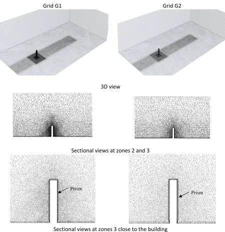
3.4.2 Grid Discretization ... 60
3.5 Results and discussions ... 63
3.5.1 Wind Flow Field ... 63
3.5.2 Mean and rms pressure coefficient distributions ... 66
3.5.3 Building Responses ... 74
3.6 Conclusions ... 81
ix
4 Enhancing wind performance of tall buildings using corner aerodynamic optimization
... 89
4.1 Introduction ... 89
4.2 Aerodynamic Optimization Procedure (AOP) ... 94
4.3 Aerodynamic optimization application examples ... 97
4.3.1 LES properties of a 2D flow (training models) ... 99
4.3.2 ANN model properties ... 101
4.3.3 LES properties of an ABL flow ... 105
4.3.4 Optimization algorithm properties ... 108
4.4 Optimization results and verification discussions... 108
4.4.1 Optimization results and discussions ... 108
4.4.2 Verification and wind load evaluation results ... 111
4.5 Conclusions ... 118
4.6 References ... 119
Chapter 5 ... 124
5 Aerodynamic shape optimization of tall buildings using twisting and corner modifications ... 124
5.1 Introduction ... 124
5.2 Aerodynamic optimization procedure (AOP) framework ... 125
5.3 Illustration example ... 126
5.3.1 CFD model properties ... 127
5.3.2 Artificial neural network (ANN) properties ... 129
5.3.3 Genetic algorithm (GA) properties ... 130
5.4 Optimization results ... 131
5.5 Conclusion ... 133
x
6 Multi-objective optimization of tall building vents for wind-induced loads reduction
... 136
6.1 Introduction ... 136
6.2 Aerodynamic Optimization Procedure (AOP) ... 139
6.3 Demonstration Optimization problems ... 141
6.3.1 LES properties of an ABL flow ... 143
6.3.2 ANN model properties ... 147
6.3.3 GA details ... 148
6.4 Single-objective optimization ... 149
6.5 Multi-objective optimization ... 153
6.6 Conclusions ... 154
6.7 References ... 155
Chapter 7 ... 160
7 Conclusions and Recommendations ... 160
7.1 Summary ... 160
7.2 Main Contributions ... 160
7.3 Recommendations for future work ... 163
Appendices A ... 164
xi
Table 2-1 Inflow generation methods ... 14
Table 2-2 Parameters used for generating velocity field for urban terrain exposure ... 18
Table 2-3 Properties of the examined building ... 31
Table 2-4 Computational domain dimensions ... 32
Table 2-5 Properties of the employed grids ... 34
Table 2-6 Parameters used in the LES ... 36
Table 3-1 Scope and the main findings of previous studies focused on building responses .. 51
Table 3-2 Parameters used for generating velocity field ... 56
Table 3-3 Parameters used in the LES ... 60
Table 3-4 Properties of the employed grids ... 61
Table 3-5 Grid size, wind angle of attack and building configuration for the study cases ... 63
Table 3-6 Dynamic properties of the examined building ... 79
Table 4-1 Scope and main findings of previous studies focused on local mitigations ... 91
Table 4-2 Examples for the analytical models and their formulas ... 102
xii
Figure 1-1 Examples of tall building local (corner) mitigations ... 3
Figure 1-2 Examples of tall buildings global mitigations ... 3
Figure 2-1 Recycling technique (Lund et al. 1998) ... 13
Figure 2-2 coherency function between velocities at points 1 and 2 resulting from the DRFG technique ... 19
Figure 2-3 Sample velocity time history resulting from the DRFG (Huang et al. 2010) and their spectral plots ... 20
Figure 2-4 Velocity time history resulting from DRFG using a single fm of 20 Hz and their spectral plots ... 21
Figure 2-5 Velocity time history resulting from CDRFG and their spectral plots using one fm = 20 Hz (Equation 6 using updated fn,m, pim,n and qim,n expressions) ... 22
Figure 2-6 Sample velocity time history resulting from CDRFG and their spectral plots ... 23
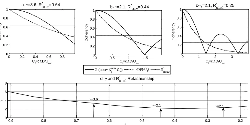
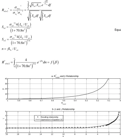
Figure 2-7 Fitting process for coherency function resulting from CDRFG technique for different Ru1u2* values (a) to (c) , and (d) relationship between Ru1u2* and γ ... 26
Figure 2-8 Relationship between Ru1u2*, β and γ ... 27
Figure 2-9 CDRFG technique flow chart ... 28
Figure 2-10 Velocity time histories and coherency functions at points 1 and 2 resulting from the CDRFG technique ... 30
Figure 2-11 Target and resulting coherency functions for different separation distances ... 30
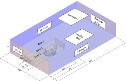
Figure 2-12 Boundary conditions and domain dimensions ... 32
Figure 2-13 Dimensions of different mesh zones ... 34
xiii
Figure 2-16 Surfaces of equal vorticity magnitude ... 38
Figure 2-17 Plots for base moments around the x-axis (across wind), y-axis (along-wind) and z-axis (torsional) obtained from LES using CDRFG technique ... 39
Figure 2-18 Spectra of the base moments ... 40
Figure 2-19 Peak top floor displacements ... 41
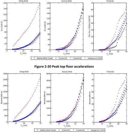
Figure 2-20 Peak top floor accelerations ... 42
Figure 2-21 Peak base moments ... 42
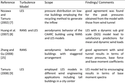
Figure 3-1 CDRFG technique flow chart (Aboshosha et al. [12], reproduced with permission) ... 55
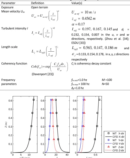
Figure 3-2 profiles measured from the wind tunnel and the fitted profiles for CFD ... 56
Figure 3-3 Wind tunnel test configurations (Dragoiescu et al. [32], reproduced with permission) ... 57
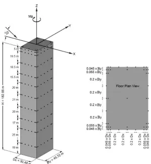
Figure 3-4 CAARC standard full-scale dimensions and pressure tap locations ... 58
Figure 3-5 Computational domain dimensions and boundary conditions ... 60
Figure 3-6 Comparison between grids G1 and G2 (Configuration 1 – isolated case) ... 62
Figure 3-7 Grid G1* used for the surrounded building model (Configuration 2 –complex surrounding). ... 62
Figure 3-8 Instantaneous velocity magnitude contours ... 64
Figure 3-9 Instantaneous vorticity magnitude contours ... 64
Figure 3-10 Mean velocity magnitude and quasi-streamlines ... 65
xiv
Figure 3-13 Comparing mean Cp distribution of current study with BLWT from literature .. 68
Figure 3-14 Comparing rms Cp distribution of current study with BLWT from literature .... 69
Figure 3-15 Contour distribution of mean Cp over front and back faces of CAARC building obtained from current study and literature ... 71
Figure 3-16 Contour distribution of rms Cp over front and back faces of CAARC building obtained from current study and literature ... 72
Figure 3-17 mean pressure coefficient distribution over building faces ... 73
Figure 3-18 fluctuating pressure coefficient (rms) distribution over building faces ... 74
Figure 3-19 Base moments around the x-axis (along-wind), y-axis (across-wind) and z-axis (torsional) ... 75
Figure 3-20 Spectra of the base moments ... 77
Figure 3-21 Peak top floor displacements ... 79
Figure 3-22 Peak top floor accelerations ... 80
Figure 3-23 Peak base moments ... 81
Figure 4-1 Examples of tall building corner mitigations ... 90
Figure 4-2 Framework of Aerodynamic Optimization procedure (AOP) ... 95
Figure 4-3 Flowchart of the genetic algorithm optimization process ... 97
Figure 4-4 Geometric parameters of the study cross-section ... 99
Figure 4-5 Training samples for Artificial Neural Network model ... 100
xv
instantaneous velocity vector contour ... 101
Figure 4-8 Regression plots for different sizes of training samples; (a) 50 samples (b) 100
samples (c) 125 samples (d) 150 samples (e) 175 samples and (f) 200 samples ... 104
Figure 4-9 (a) Error distribution and (b) regression plot for the ANN model ... 104
Figure 4-10 (a) velocity, (b) turbulence intensity and (c) turbulence length scale profiles used
for inflow generation using CDRFG technique ... 106
Figure 4-11 Computational domain dimensions and boundary conditions ... 106
Figure 4-12 Grid resolution utilized for the ABL flow simulations ... 107
Figure 4-13 Spectra of the base moments in the (a) along-wind and (b) across-wind directions
... 107
Figure 4-14 Fitness curves for the (a) drag and (b) lift optimization examples ... 109
Figure 4-15 Selected cross-sections from (a) drag and (b) lift optimization examples ... 110
Figure 4-16 Surface plot for the ANN model of the (a) mean drag and (b) fluctuating lift
coefficients ... 110
Figure 4-17 Mean velocity & Cp distribution for the drag optimal (D4) & near optimal (D1)
cross-sections ... 112
Figure 4-18 Instantaneous velocity field & Cp distribution for the lift optimal (L4) & near
optimal (L1) cross-sections ... 112
Figure 4-19 Normalized mean drag coefficients and of cross-sections from drag optimization
using (a) 2D flow and (b) ABL flow ... 113
Figure 4-20 Normalized Fluctuating lift coefficients of cross-sections from lift optimization
xvi
from drag optimization and (b) around y-axis (across-wind) of cross-sections from lift
optimization ... 115
Figure 4-22 Base moments spectra (a) around x-axis (along-wind) of cross-sections from drag optimization and (b) around y-axis (across-wind) of cross-sections from lift optimization ... 116
Figure 4-23 (a) Peak top floor displacement, (b) acceleration and (c) base moments in the along-wind direction of cross-sections from drag optimization ... 117
Figure 4-24 (a) Peak top floor displacement, (b) acceleration and (c) base moments in the across-wind direction of cross-sections from lift optimization... 118
Figure 5-1 Framework of the aerodynamic optimization procedure (AOP) ... 126
Figure 5-2 Geometric parameters (length in meters and angle in degree) ... 127
Figure 5-3 (a) velocity, (b) turbulence intensity and (c) turbulence length scale profiles used for inflow generation using CDRFG technique ... 128
Figure 5-4 Grid resolution utilized for the LES analysis ... 128
Figure 5-5 Normalized moment coefficient time history in the along-wind direction for sample of shapes ... 129
Figure 5-6 a) Error distribution and b) Regression plot for the ANN ... 130
Figure 5-7 Fitness curves for the optimization example ... 131
Figure 5-8 (a) Mean velocity and pressure coefficient contour (b) Normalized moment coefficient in the along-wind direction for the square and optimal cross-sections ... 132
Figure 6-1 Examples of global mitigations of tall building ... 139
Figure 6-2 flowchart of the aerodynamic optimization procedure (AOP) ... 140
xvii
Figure 6-5 (a) mean velocity, (b) turbulence intensity and (c) turbulence length scale profiles
used for inflow boundary condition ... 144
Figure 6-6 Vorticity visualization for a training model ... 145
Figure 6-7 Grid resolution utilized for the ABL flow simulations ... 145
Figure 6-8 Time histories of moment coefficient about (a) x- and (b) y-axis for different geometric samples ... 146
Figure 6-9 Peak moment coefficient about (a) x- and (b) y-axis for different geometric samples ... 146
Figure 6-10 Randomly selected training samples for Artificial Neural Network model ... 147
Figure 6-11 Regression plot for the ANN model estimating (a) CM x, and (b) CM y, ... 148
Figure 6-12 Error distribution of the ANN model ... 148
Figure 6-13 Fitness curves for the (a) CM x, and (b) CM y, optimization ... 150
Figure 6-14 Surface plot for the ANN model of the peak moment coefficient about x-axis 151 Figure 6-15 Mean wind field and Cp distribution for the (a) basic, (b) optimal 1; and (c) optimal 2 building shapes ... 152
Chapter 1
1
Introduction
1.1
Background
New generations of tall buildings are becoming increasingly taller, flexible and slender
primarily driven by novel developments in design methods and new construction materials
and techniques. This in turn makes tall buildings more sensitive to lateral loads such as
wind. In addition, there is a need to lower the building weight in order to decrease the
gravity loads to control the inertial forces developed by earthquake. This further contributes
to an increase in the wind-induced forces and motions. As a result, wind-induced loads and
motions typically govern the design of the lateral load resisting systems in tall buildings.
The outer shape of the building is one of the main parameters that affect these loads and
responses. The dependence of the wind load on the building shape makes the
generalizations of wind load for tall buildings almost impossible, because every complex
shape and surroundings produce a unique set of design wind loads. On the other hand, this
dependency on the shape provides a unique opportunity to reduce the wind load through
outer shape modifications.
In general, controlling wind-induced loads and vibrations can be achieved through three
approaches that include: (1) utilizing sufficient structural components and external
damping systems, (2) introducing aerodynamic mitigations for the outer shape of a
building, or (3) combining the previous two approaches by improving both structural
components and aerodynamic performances of the building. The first approach sacrifices
avoid changing the building outer shape. The second approach saves these expenses by
reducing the applied wind load through aerodynamic mitigation. It should be noted that, in
many cases, meeting the strength and serviceability requirements cannot be satisfied unless
both structural and aerodynamic improvements (third approach) are used. For this reason,
almost all recently built super tall buildings have applied aerodynamic mitigations either
locally (at the corner shapes) or globally (along the height of the building). Many
researchers have reported that careful modification of the shape of the corners can provide
better aerodynamic performance (Kwok 1988, Kareem et al. 1999, Tamura and Miyagi
1999, Carassale et al. 2014). “Local Shape Mitigation” of tall buildings focuses on the
change of the corner shapes to enhance the aerodynamic performance (Figure 1-1). The
main advantage of this type of mitigation is that the effect on the architectural and structural
concept of the structure is limited. Detailed literature on “Local Shape Mitigation” is
provided in Chapter 4 of this thesis. In contrast, “Global Shape Mitigation” has a
considerable effect on the architectural and structural design because the mitigations affect
the whole height and width of the building (e.g. twisting, tapering and opening) rather than
being localized at the corners (Figure 1-2). This scale of mitigation can enhance the
aerodynamic performance because a wider variety of changes is applied. “Global Shape
Figure 1-1 Examples of tall building local (corner) mitigations
Figure 1-2 Examples of tall buildings global mitigations
It can be noticed that many previous studies compared different types of mitigations based
on a single set of dimensions for each mitigation family. However, each family (of a
specific shape mitigation) can produce a wide range of aerodynamic performances based
on the selection of a different combination of mitigation dimensions. Consequently, a wider
search space (i.e. more building shape alternatives) can be explored by integrating an
Kareem et al. (2013a, b and 2014) introduced an approach for tall building corner
optimization to reduce drag and lift by adopting two-dimensional CFD models. This
approach is useful to overcome the computational cost associated with the iterative
procedure required for optimization. Bernardini et al. 2015 investigated the efficiency of
utilizing Kriging model as a surrogate model for the objective function evaluation. The
utilization of a surrogate model reduced the computational time. In these studies, Unsteady
Reynolds-Averaged Navier–Stokes (URANS) equations were used. Although these
studies developed a very promising and useful approach for building aerodynamic
optimizations, some limitations are observed. For example, (i) wind directionality effect
is not considered, (ii) low-order CFD models are used to evaluate shape alternatives,
although wind performance assessment usually requires the use of high accuracy CFD- or
BLWT-based evaluations (iii) only two-dimensional flow was used to assess various
cross-sections. Using these novel approaches, it is possible to infer the relative performance of
the various geometric alternatives (i.e. comparing alternatives) adopting the reduced order
2D simulations. A similar conclusion was also reported by Tamura and Miyagi 1999. Thus,
adopting a simplified low order simulation can significantly reduce the analysis accuracy
that may affect the conclusions observed under such simplified scenarios. Particularly
when simulating the turbulent atmospheric boundary layer (ABL) flow and its interaction
with a tall building. These complex interactions can be realistically captured through LES
as reported by Nozawa and Tamura (2002), Dagnew and Bitsuamlak (2013 and 2014).
It is to be noted that the accuracy of LES depends on the proper selection of the inflow
to the Keating et al. (2004) inflow boundary condition (IBC) can be generated using three
methods (i) precursor database (Bitsuamlak and Simiu 2010, Liu and Pletcher 2006), (ii)
recycling method (Lund et al. 1998; Nozawa and Tamura 2002, Aboshosha et al. 2015),
and (iii) synthesizing the turbulence (Kondo et al. 1997; Huang et al. 2010; Smirnov et al.
2001). The first two methods require prior simulations to generate the inflow which can be
computationally expensive compared to the synthesizing the turbulence method. Huang et
al. (2010) suggested the discrete random flow generation (DRFG) method to produce
turbulent velocity field that has turbulent spectra close to the target ABL flow
characteristics that forms also the basis for current study. Castro et al. (2011) proposed a
modification to the DRFG method to obtain velocity field that had a better match with the
target spectra. Generally, the DRFG method is able to generate turbulent spectra that is
close to the target, maintain the spatial correlation among the resulting velocities, and can
easily be implemented in parallel computing environment. However, there are other
additional important conditions that needs to be satisfied by the generated inflow for wind
engineering applications such as maintaining the continuity equation and the proper
coherence among the velocities (Davenport 1993). This include maintaining proper
correlations among the turbulent velocities within different frequencies as indicated by
Davenport (1993) and Kijewski and Kareem (1998). Another important condition is
modeling the turbulent spectra to be exactly similar as the target flow. A further detailed
review about inflow generation techniques is presented in Chapter 2 of this thesis.
1.2
Research Gap
As discussed earlier, a significant improvement in the aerodynamic performance can be
achieved by modifying the outer shape of a tall building. Majority of previous studies
compare shape alternatives based on one geometry for each mitigation family leading to
an ad hoc solution rather than an optimal solution. Thus, for further aerodynamic
improvement, the aerodynamic assessment method (i.e. Wind Tunnel or CFD) needs to be
coupled with an optimization technique. This will result in exploring wider search space
towards the optimal building shape. It is also required that the optimization process to be
computationally affordable to overcome the computationally expensive CFD analyses
without affecting the accuracy of the numerical modelling. Finally, since the accuracy of
the CFD analysis depends on the proper matching to the target inflow profiles and statistics,
a more accurate inflow technique needs to be developed that satisfy the coherency among
velocities and the continuity equation (i.e. diversion-free).
1.3
Scope of Thesis
The thesis aims to address the research gaps mentioned in the above section. As such, the
objectives of the thesis are:
1. Developing an aerodynamic optimization procedure that is capable of identifying
the optimal building shape for a selected mitigation type.
2. Examining the proposed optimization procedure for “Local Shape Mitigations”
and “Global Shape Mitigations”.
3. Adopting the proposed optimization procedure to conduct single-objective and
multi-objective optimization problems.
4. Developing accurate numerical models to evaluate wind loads though LES and
novel inflow generation technique that satisfy the target velocity and turbulence
profiles in addition to other flow statistics such as coherency and continuity.
5. Validating the numerical wind load evaluation using experimental work from
wind tunnel test and other numerical studies.
1.4
Organization of thesis
This thesis has been prepared in an “Integrated-Article” format. In Chapter 1, a review of
using CFD is provided. These objectives are addressed in detail in the following five
chapters.
1.4.1
Consistent inflow turbulent generator for LES evaluation of
wind-induced responses for tall buildings
This chapter discusses a new turbulent inflow generator technique that can be used as
inflow boundary condition for LES based on synthesizing random divergent-free turbulent
velocities. The accuracy of the proposed technique to produce turbulent velocities with
proper spectra and coherency function is assessed in comparison with typical ABL flow
characteristics obtained from literature. Further, its appropriateness to evaluate
wind-induced response for tall building is assessed by employing the proposed technique as inlet
boundary condition for LES of the ABL flow around a typical tall building that was
previously tested in a boundary layer wind tunnel.
1.4.2
LES evaluation of wind-induced responses for an isolated
and a surrounded tall building
In this chapter, the aerodynamic response of a standard tall building (commonly known as
the CAARC model) is investigated using LES. The LES employs the Consistent Discrete
Random Flow Generation (CDRFG) technique to generate the inflow boundary condition.
The building aerodynamic behavior is investigated for two configurations (an isolated
building and a building with complex surrounding buildings) and the results are compared
with a previous wind tunnel test.
1.4.3
Enhancing wind performance of tall buildings using corner
aerodynamic optimization
This chapter presents building corner aerodynamic optimization procedure (AOP) to
reduce the wind load, by coupling an optimization algorithm, Large Eddy Simulation
(LES) and an artificial neural network (ANN) based surrogate model. Two aerodynamic
optimization examples focusing on drag and lift minimization that consider wind
Mitigations”, two-dimensional inflow is utilized in examining different building
cross-sections. The aerodynamic performance of optimal shapes is compared to other near
optimal shapes to elaborate the improvement achieved throughout the optimization
process.
1.4.4
Aerodynamic shape optimization of tall buildings using
twisting and corner modifications
In this chapter, improving the aerodynamic performance of tall buildings is conducted by
adopting the AOP to reduce the along-wind base moment by helical twisting and corner
modifications of a tall building. Three-dimensional LES of a synoptic inflow is used to
assess different shape alternatives during the optimization process.
1.4.5
Multi-objective optimization of tall building vents for
wind-induced loads reduction
This chapter discusses the utilization of the AOP to conduct multi-objective optimization
problem (considering more than one objective function) by optimizing the introduction of
three openings to a standard tall building named the Commonwealth Advisory
Aeronautical Research Council (CAARC). The optimization process aims to reduce both
wind-induced base moments by changing the aspect ratio of the openings and the distances
between successive openings.
1.5
References
Aboshosha H, Bitsuamlak G, El Damatty A. LES of ABL flow in the built-environment using roughness modeled by fractal surfaces. Sustainable Cities and Societies 2015; 19, 46-60.
Bernardini E, Spence S, Wei D, Kareem A. Aerodynamic shape optimization of civil structures: A CFD-enabled Kriging-based approach, Journal of Wind Engineering and Industrial Aerodynamics 2015; 144, 154-164.
Carassale L, Freda A, Marrè-Brunenghi M. Experimental investigation on the aerodynamic behavior of square cylinders with rounded corners. Journal of Fluids and Structures 2014; 44, 195-204.
Castro, G.H., Paz, R.R., Sonzogni, V.E. 2011. Generation of turbulent inlet velocity conditions for large eddy simulations. Mecánica Computacional, 2275-2288.
Dagnew A, Bitsuamlak GT. Computational evaluation of wind loads on buildings: a review, Wind and Structures 2013; 16(6), 629-660.
Dagnew A, Bitsuamlak GT. Computational evaluation of wind loads on standard tall building using a large eddy simulation, Wind & Structures 2014; 18(5), 567-598.
Davenport, A.G.1993.How can we simplify and generalize wind loads? Presented at the Third Asia-Pacific Symposium on Wind Engineering, Keynote Lecture, December13–15, Hong Kong.
Huang S, Li Q, Wu J. A general inflow turbulence generator for large eddy simulation. Journal of Wind Engineering and Industrial Aerodynamics 2010; 98, 600-617.
Kareem A, Spence SMJ, Bernardini E, Bobby S, Wei D. Using computational fluid dynamics to optimize tall building design. CTBUHJ. (III) 2013a; 38-42.
Kareem A, Bernardini E, Spence SMJ. Control of the Wind Induced Response of Structures. Springer, Tokyo, Japan 2013b, 377-410 (Chapter14).
Kareem A, Bobby S, Spence SMJ, Bernardini E. Optimizing the form of tall buildings to urban environments. In: CTBUH 2014 International Conference 2014.
Kareem A, Kijewski T, Tamura Y. Mitigation of motions of tall buildings with specific examples of recent applications. Wind and structures 1999; 2(3), 201-251.
Keating A, Piomelli U, Balaras E, Kaltenbach HJ. A priori and a posteriori tests of inflow conditions for large-eddy simulation. Physics of Fluids 2004; 16, 4696.
Kijewski T., Kareem A. 1998. Dynamic wind effects: a comparative study of provisions in codes and standards with wind tunnel data. Wind and Structures, 1(1), 77-109.
Kondo K, Murakami S, Mochida A. Generation of velocity fluctuations for inflow boundary condition of LES. Journal of Wind Engineering and Industrial Aerodynamics 1997; 67-68, 51-64.
Kwok KCS. Effects of building shape on wind-induced response of tall buildings. Journal of Wind Engineering and Industrial Aerodynamics 1988; 28, 381-90.
Liu KL, Pletcher RH. Inflow conditions for the large eddy simulation of turbulent boundary layers: a dynamic recycling procedure. Journal of Computational Physics 2006; 219 (1), 1-6.
Nozawa K, Tamura T. Large eddy simulation of the flow around a low-rise building immersed in a rough-wall turbulent boundary layer. Journal of Wind Engineering and Industrial Aerodynamics 2002; 90, 1151-1162.
Smirnov R, Shi S, Celik I. Random flow generation technique for large eddy simulations and particle-dynamics modeling. Journal of Fluids Engineering 2001; 123, 359-371.
Tamura T, Miyagi T. The effect of turbulence on aerodynamic forces on a square cylinder with various corner shapes. Journal of Wind Engineering and Industrial Aerodynamics 1999; 83, 135-145.
Tamura, T. 2010a. Application of LES-based model to wind engineering- Implementation of meteorological effects. The Fifth International Symposium on Computational Wind Engineering, Chapel hill, NC, May 23-27.
Tamura, T. 2010b. LES for aerodynamic characteristics of a tall building inside a dense city district”, The Fifth International Symposium on Computational Wind Engineering, Chapel hill, NC, May 23- 27.
Chapter 2
2
Consistent inflow turbulent generator for LES
evaluation of wind-induced responses for tall
buildings
2.1
Introduction
With encouraging development trends, both in software and hardware technology, the cost
of conducting Large Eddy Simulation (LES) for wind engineering applications is becoming
computationally affordable. This is also reflected through an increased number of
publication that uses LES for variety of wind engineering applications. To give few
examples, recently Dagnew and Bitsuamlak (2014) and Daniels et al. (2013) applied LES
to evaluate wind load on standard tall buildings. Nozu et al. (2008), Tamura (2010a, b),
Huang and Li (2010), Lim et al. (2009) employed LES to study building aerodynamics.
Aboshosha et al. (2015) used LES to characterize the turbulence structure of downburst.
Abdi and Bitsuamlak (2014) used LES among other turbulence models to characterize flow
over topography. Tominaga and Stathopoulos (2010, 2011) used LES to study the pollution
dispersion around a building and street canyon, respectively, Gousseau et al. (2013) used
LES to study pollution dispersion in a city center, and Jiang et al. (2013) used LES to study
natural ventilation.
The importance of defining proper inflow boundary condition (i.e. turbulence) while using
LES was extensively discussed by various researchers (Sagaut et al. 2003; Tutar and Celik
2007; Xie and Castro 2008; Tominaga et al. 2008; Dagnew and Bitsuamlak 2013). The
inflow condition should satisfy specific spectra, correlations and magnitudes. To this end,
several techniques are available in the literature (Kondo et al. 1997; Smirnov et al. 2001;
Jarrin et al. 2006; Tamura 2000). Keating et al. (2004) classified the techniques used to
generate inflow turbulence for LES into three categories, which are (i) precursor database,
(ii) recycling method and (iii) synthetic turbulence. Liu and Pletcher (2006) provided a
simulation of the flow around a targeted zone is conducted in two stages. In the first stage,
a parent simulation for the incoming wind upstream to the zone of interest is conducted to
obtain incoming temporal and spatial turbulent velocities. These turbulent velocities are
saved in a database and used for the second simulation stage, where the flow is focused on
the zone of interest. Although this method is employed previously in wind engineering
application, it is computationally costly and not preferable unless the first simulation stage
already exists and turbulent velocity database is available (Bitsuamlak and Simiu 2010).
Lund et al. (1998) used the recycling method to generate inflow velocities for smooth
terrains. Nozawa and Tamura (2002) extended Lund’s method and employed it with rough
terrains. Similar to precursor database method, computational domain is divided into two
in the recycling method: (i) the driver domain and (ii) the calculation domain. In the driver
domain, the flow is recycled over a short domain until the flow becomes statistically stable.
Flow characteristics on a mapping plane is stored and used as the inflow condition for the
calculation domain as illustrated in Figure 2-1. The main drawback of the recycling method
is that resulting inflow characteristics are dependent on the roughness elements used at the
floor of the driver domain. Unless shape and distribution of the roughness elements leading
to targeted flow characteristics (i.e. terrain exposure) are known, this method cannot be
used (Tamura 2008). Aboshosha (2014) suggested a technique suitable for recycling
method that allows for simulating any targeted terrain exposure through the usage of fractal
surfaces. This technique has been utilized by Aboshosha et al. (2015) while studying
downburst flows for various terrain exposures. The drawback associated with all recycling
methods is the requirement for a parent simulation using a driver domain that makes the
turbulent inflow generation time consuming compared with other methods such as
synthesizing inflow turbulence (Tamura 2008). Synthesizing inflow turbulence does not
require costly prior simulations, making it a more robust approach provided that the target
Figure 2-1 Recycling technique (Lund et al. 1998)
According to Huang et al. (2010), synthesizing inflow turbulence techniques can be
classified into two main groups. The first group include the work of Hoshiya (1972),
Iwatani (1982), Maruyama and Morikawa (1994), and Kondo et al. (1997). This group uses
a weighted amplitude wave superposition method (WAWS) which results in a turbulent
velocity field that satisfies both the targeted power and cross spectra.
The drawback of this method is that resulting turbulent field is not dependent on the
computational grid used, thus, does not satisfy the continuity condition of the flow (i.e.
divergence free is not guaranteed). This would require enormous effort from the solver to
correct the assigned flow field and enforce the continuity (Tamura 2008). Kondo et al.
(1997) employed the method originally developed by Shirani et al. (1981) to make the
generated inflow divergent free. However, the step involved to maintain the divergence
free criterion alters the targeted statistical characteristics. Kim et al. (2013) suggested to
introduce the turbulent field on a vertical plane near (rather than at) the inlet and relied on
the pressure-correction to maintain the divergence free criterion. This reduced degradation
of the statistical characteristics compared to when the field is introduced right at the inlet.
Daniels et al. (2014) employed this method to estimate peak pressures on a typical tall
building and reported that the method is rapid and led to encouraging results. The second
group include the work of Kraichnan (1970), Li et al. (1994), Bechara et al. (1994), Fung
et al. (1992), Smirnov et al. (2001), Klein et al. (2003), and Batten et al. (2004). This group
generates divergent-free velocity field with Gaussian spectra and is usually referred as
commercial CFD software. Unfortunately, turbulent spectra in the atmospheric boundary
layer (ABL) is different from Gaussian spectra (Lumley and Panofsky 1964), thus making
RFG method not suitable for wind engineering application. Huang et al. (2010) suggested
the discrete random flow generation (DRFG) method to produce turbulent velocity field
that has turbulent spectra close to the target ABL flow characteristics that forms also the
basis for current study. Castro et al. (2011) proposed a modification to the DRFG method
to obtain velocity field that had a better match with the target spectra. Generally, the DRFG
method is able to generate turbulent spectra that is close to the target, maintain the spatial
correlation among the resulting velocities, and can easily be implemented in parallel
computing environment. Table 2-1 summarizes the methods available in the literature to
generate the inflow condition.
Table 2-1 Inflow generation methods
Group/ Subgroup Study Comments
Precursor database Bitsuamlak and Simiu 2010
Two steps (i) parent simulation for the incoming wind upstream and, (ii) second simulation for the targeted zone
Recycling method
Lund et al. (1998) Generate inflow for smooth terrains
Nozawa and Tamura (2002) Generate inflow for rough terrains
Aboshosha (2014)
Simulated any targeted terrain exposure through the usage of fractal surfaces
Synthetic turbulence
WAWS
Hoshiya (1972), Iwatani (1982),
Maruyama and Morikawa
(1994), Kondo et al. (1997)
Turbulent field is not dependent on the computational grid, thus, does not satisfy the continuity condition
Kondo et al. (1997), Kim et al. (2013)
Suggested methods to satisfy the divergence free criterion but affects the targeted statistical properties, coherency among the velocities is not maintained
RFG
Kraichnan (1970), Li et al. (1994), Bechara et al. (1994), Fung et al. (1992), Smirnov et al. (2001), Klein et al. (2003), Batten et al. (2004)
Gaussian spectra, which is not compatible with the spectra in the ABL
Huang et al. (2010) and Castro et al. (2011)
Turbulent spectra that is close to the
target, maintain the spatial
parallel computing environment, coherency among the velocities is not maintained.
However, there are other additional important conditions that needs to be satisfied by the
generated inflow for wind engineering applications such as maintaining the proper
coherence among the velocities (Davenport 1993). This include maintaining proper
correlations among the turbulent velocities within different frequencies as indicated by
Davenport (1993) and Kijewski and Kareem (1998). Another important condition is
modeling the turbulent spectra to be exactly similar as the target flow. Unfortunately, these
conditions are not met by the DRFG method, as will be illustrated in the following section.
The current study focuses on modifying the DRFG method to maintain the proper
coherency among the resulting turbulent velocities. The modified method is named
consistent DRFG (or CDRFG) method. In the following sections of the paper presents brief
discussion on the original DRFG method as suggested by Huang et al. (2010) and
highlights the rational that led to the need to improve the spectra and coherency function
of inflow turbulence to better fit the target flow characteristics (section 2). Proposed
modifications to the DRFG technique (CDRFG technique) enabled robust modeling of the
spectra and the coherency function and are presented in section 3. In section 4, both the
new CDRFG and the original DRFEG techniques are applied as inflow boundary
conditions of LES to evaluate wind-induced responses of a typical tall building. The
numerical results are then compared with aerodynamic data obtained from a boundary layer
wind tunnel test for assessing their respective performance.
2.2
Discrete random inflow generation
As mentioned earlier, Huang et al. (2010) proposed the discrete random flow generation
(DSRG) technique to generate turbulent velocity field that satisfies the targeted turbulent
spectra and spatial correlations. The technique is based on discretizing power spectra of
velocities into M number of segments and generate wind field within each of these
segments using the original random flow generation (RFG) technique (Kraichnan 1971 and
arbitrary distribution. According to Huang et al. (2010), turbulent velocity field, ui(xj,t)
can be generated using Equation 2-1Equation 6-1.
, , , ,
, ,
1 1
( , ) cos . 2. sin . 2.
M N m n m n m m n m n m j j
i j i j n m i j n m
m n
u x t p k x
f t q k x
f tEquation 2-1
where uirepresent longitudinal u, transverse v, and vertical w velocities, respectively; j=1,
2 and 3 represent x, y and z directions, respectively; M is the number of spectral segments;
N is the number of random frequencies within each segment; pim n, and
,
m n i
q are parameters
defined in Equation 2-2; fn m, is a normally distributed random number with 0 mean and
m
f standard deviation; m n,
j
k are coordinates of a uniformly distributed points on a sphere
with a unit radius that satisfy Equation 2-3 to maintain the divergence free condition; xjm
is a non-dimensional location coordinate where the velocity is being generated and is
defined by Equation 2-4, where xj is the location coordinate in the j direction.
2 , , , 2 , , , 2 , 12 ( ).
1
1 1
2 ( ).
1 m n i
m n m n
i i ui m
m n i
m n m n
i i ui m
m n i
r
p sign r S f f
N r
q sign r S f f
N r
Equation 2-2
where Sui(fm)is the spectra in the direction i at the frequency fm and ,
m n i
r is a normally
distributed random number with zero mean and unit standard deviation, fm. is bandwidth
defining the spectra segment.
, , , . , , , . . . . . 0 0 1
m n m n m n m n
x y z x
m n m n m n m n
x y z y
m n m n m n m n
x y z z
p p p k
q q q k
k k k k
m j
j m
j
x x
L
Equation 2-4
The parameter Ljm in Equation 2-4 characterizes the spatial correlations between the
generated velocity field. Huang et al. (2010) suggested to relate the parameter m j
L to the
integral length scale of turbulenceC LL. uj, where CL is a factor ranging between 1 and 2,
with an average value of 1.5. They compared the spatial correlation of the generated
velocity vectors with the target and found that a value of 1.5 Luj leads to a good agreement.
It should be mentioned that Huang et al. (2010) uses a frequency independent parameter
m j
L , which is expected to result in a frequency independent correlation (i.e. same
correlation for all frequencies). This contradicts with the fact that large eddies (with low
frequencies) have higher correlations than small eddies (with high frequencies) (Davenport
1967 and 1993). It is to be noted that maintaining proper frequency-dependent correlations
is very important while estimating wind-induced responses of flexible structures such as
tall buildings and long span bridges (Davenport 1993). Another disadvantage of DRFG
technique is that spectra of the resulting turbulent deviates from the target ABL flow
statistics (Castro et al. 2011). To explain these limitations more specifically, DRFG
technique (Equations 1-4) is used to generate turbulent velocity field for an urban terrain
defined by using m j
L = 1.5 Luiand parameters summarized in Table 2-2. These parameters
are chosen to match the urban exposure used in the boundary layer wind tunnel experiments
reported by Kijewski and Kareem (1998) and Zhou et al. (2003). More specifically mean
velocity, turbulent intensity and longitudinal integral scale of turbulence were adopted
from Zhou et al. (2003). The target coherency function (expression given in Table 2-1) is
adopted from Davenport (1993). Other parameters (listed in Table 2-1) that are required
Table 2-2 Parameters used for generating velocity field for urban terrain exposure
Parameter Definition/ Value
Exposure Urban
Mean velocity Uav
av av ref ref z U U z , av ref
U =10 m/s, zref= 0.364 m, α=0.326
Turbulent intensity I
dj j refj ref z I I z
where Irefj= 0.208, 0.182, 0.152 and dj = 0.191, 0.123, 0.005 in the u, v and w
directions, respectively. (Zhou et al. 2003; ESDU 2001)
von Karman turbulent spectra
Su, Sv, Sw
2 5/6 24( ) /
1 70.8 /
u av u av u
u av I U L U S fL U
2 2 11/6 24( ) / 1 188.4 2 /
1 70.8 2 /
v av v av v av
v
v av
I U L U fL U
S fL U
2 2 11/6 24( ) / 1 188.4 2 /
1 70.8 2 /
w av w av w av
w
w av
I U L U fL U
S
fL U
where
j j refj refL z L L z
, LrefJ = 0.302, 0.0815, 0.0326 m,
j
= 0.473, 0.881, 1.539, in x, y, z directions respectively; zrefL=0.254 m
Coherency function
Other parameters
( )exp
j m j m
av
C f dx Coh f
U (Davenport 1993) where C
j is coherency decay
constant.
fm min=1.0 hz, fm max= 100 hz, Δf=1.0 hz, M=100, N=50
Figure 2-2 shows the coherency function between resulting two velocities vectors at
heights of 0.1 m and 0.3 m from ground. The resulting coherency function is compared
with the targeted coherency function suggested by Davenport (1993) (given in Table 2-1)
As shown in Figure 2-2, the coherency produced by adopting the DRFG technique is
frequency independent and fails to capture the decaying distribution with the frequency
increase. This leads, for example, to an overestimation of the forces acting on structures
that has fundamental frequency greater than fint, shown in Figure 2-2.
Figure 2-2 coherency function between velocities at points 1 and 2 resulting from the DRFG technique
Figure 2-3 shows the velocity and the spectra plots at point 2 (located at a height of 0.3 m
from ground), in the longitudinal, transverse and vertical directions compared with von
Karman spectra. The same figure also includes the smoothed spectra of the resulting
velocities (i.e. after applying a moving average) which allows for an easier comparison
with the target spectra. As indicated from the figure, the resulting spectra from DRFG do
not match the target spectra at low frequencies. Similar observation was also reported by
Castro et al. (2011). Such a discrepancy in the resulting spectra can lead to erroneous
wind-induced structural responses, especially if this discrepancy occurs close to the natural
frequencies of the structure. In the following section, proposed solutions to address the
discrepancies both in the coherency and the spectra produced while using DRFG technique
are presented.
0 1 2 3 4 5 6
-5 0 5
u 1 (m/s)
time (s) ve lo ci ty m /s
0 1 2 3 4 5 6
-5 0 5
u 2 (m/s)
time (s) ve lo ci ty m /s
0 5 10 15 20 25 0 0.1 0.2 0.3 0.4 0.5 0.6 0.7 0.8 0.9 1 f(hz) C o h e re n cy Coherency(u 1, u2)
20
Figure 2-3 Sample velocity time history resulting from the DRFG (Huang et al. 2010)
and their spectral plots
2.3
Consistent discrete random inflow generation
(CDRFG)
As illustrated in the previous section, turbulent velocities generated using DRFG technique
have some coherency and spectra discrepancies compared to the target flow statistics
observed in ABL flows. These limitations shall be addressed while using the technique to
evaluate wind-induced response of structures. Proposed enhancements to DRFG technique
are presented in this section. The proposed solutions to correct the inflow spectra are
presented first, followed by the proposed enhancements for producing consistent
coherency in the velocity field. From here after the modified technique will be referred as
consistent discrete random flow generation (CDRFG) technique, as it generates consistent
turbulent velocities (i.e. having spectra and coherency function that match the ABL flow
statistics) as will be shown later in this section.
2.3.1
Consistent wind spectra
According to Huang et al. (2010), turbulent velocity resulting from DRFG technique
corresponding to a frequency fm, u x t fi( j, , m), can be generated using Equation 2-5, where
the frequency fn,m is a random frequency with zero mean and fm standard deviation. Figure
2-4 illustrates the velocity records resulting from Equation 2-5using fm = 20 Hz for the
urban exposure parameters summarized in Table 2-2.
100 101 102
10-3 10-2 10-1 100 Su ( m 2s 2/h z) f (hz) DRFG DRFG (smoothed) von Karman
100 101 102
10-3 10-2 10-1 100 Sv ( m 2s 2/h z) f (hz) Spectra Su, Sv, Sw
DRFG DRFG (smoothed) von Karman
100 101 102
10-3 10-2 10-1 100 Sw ( m 2s 2/h z) f (hz) DRFG DRFG (smoothed) von Karman
0 1 2 3 4 5 6
-5 0 time (s) v (m /s)
0 1 2 3 4 5 6
, , , ,
, ,
1
( , , ) cos . 2. sin . 2.
N m n m n m m n m n m j j
i j m i j n m i j n m
n
u x t f p k x
f t q k x
f t Equation 2-5As shown in Figure 4, the resulting spectra have multiple peaks in the frequency band
ranging approximately between 0 and 3 fm. This means that DRFG technique distributes
the energy spectra for the frequency fm over a band of frequencies 0-3 fm, as opposed to
focusing the energy close to fm. This is believed to be the main reason for the spectral
discrepancy shown in Figure 2-4.
Figure 2-4 Velocity time history resulting from DRFG using a single fm of 20 Hz and
their spectral plots
In order to correct the discrepancy in the resulting spectra, it is suggested to use random
frequencies fn,m that are more focused near the frequency fm. Random frequencies fn,m
are chosen here to have a mean value of fm and a standard deviation of f
, where f is
frequency step used to represent the target spectra. The magnitude of the factors pi
m,n and qim,n is halved according to Equation 2-6 in order to compensate for the new utilized values
of frequencies fn,m. The resulting velocity and spectra obtained using the updated
expressions for fn,m, pim,n and qim,n expressions, and employing
f
=1.0 Hz, are shown in
100 101 102
10-3 10-2 10-1 100 Su ( m 2s 2/h z) f (hz) DRFG (fm=20 hz) von Karman
100 101 102
10-3 10-2 10-1 100 Sv ( m 2s 2/h z) f (hz) Spectra Su, Sv, Sw
DRFG (fm=20 hz) von Karman
100 101 102
10-3 10-2 10-1 100 Sw ( m 2s 2/h z) f (hz) DRFG (f
m=20 hz)
von Karman
0 1 2 3 4 5 6
-5 0 5
Velocities ufm,vfm,wfm (m/s)
time (s) ufm
(
m
/s)
0 1 2 3 4 5 6
-5 0 5 time (s) vfm ( m /s)
0 1 2 3 4 5 6
-5 0 5 time (s) wfm ( m /s)
f=fm f=fm
Figure 2-5. As shown in Figure 2-5, the resulting spectra are more focused around the
frequency fn,m and closer to the targeted value.
, 2, , 2 , 1 . 1 m n i
m n m n m
i i ui
m n i
r
p sign r S f
N r
, , 2 , 1 1 . 1 m n m n m
i i ui
m n i
q sign r S f
N r
Equation 2-6
Figure 2-5 Velocity time history resulting from CDRFG and their spectral plots using one fm = 20 Hz (Equation 6 using updated fn,m, pim,n and qim,n expressions)
The new expressions for fn,m, pim,n, and qim,nare used with Equation 1 to generate turbulent
velocities that has entire turbulent spectra. The resulting turbulent velocities and spectra
are shown in Figure 2-6 for a point located at height of 0.3 m. By comparing the resulting
spectra using the new expressions for fn,m, pim,n and qim,n with von Karman spectra, it can
be noticed from Figure 2-6 that the new expressions generated flow statistics very close to
the target.
100 101 102
10-3 10-2 10-1 100 Su ( m 2s 2/h z) f (hz) CDRFG (f
m=20 hz)
von Karman
100 101 102
10-3 10-2 10-1 100 Sv ( m 2s 2/h z) f (hz) Spectra Su, Sv, Sw
CDRFG (fm=20 hz) von Karman
100 101 102
10-3 10-2 10-1 100 Sw ( m 2s 2/h z) f (hz) CDRFG (fm=20 hz) von Karman
0 1 2 3 4 5 6
-1 0 1
Velocities ufm,vfm,wfm (m/s)
time (s) ufm
(
m
/s)
0 1 2 3 4 5 6
-1 0 1 time (s) vfm ( m /s)
0 1 2 3 4 5 6
23
Figure 2-6 Sample velocity time history resulting from CDRFG and their spectral plots
2.3.2
Correction for the coherency function
As discussed earlier, the DRFG technique leads to unrealistic coherency function that is
frequency independent. To address this shortcoming, it is proposed to relate the parameter
m j
L , which characterizes the correlations to the frequency, fm, in accordance with Equation
2-7. . . m av j j m U L C f Equation 2-7
where Uav is the mean velocity, fm is the frequency at segment m, is a tuning factor, Cj
is the coherency decay constant and j=1, 2, and 3 represents longitudinal, transverse and
vertical directions, respectively.
The expression given by Equation 2-7 requires the tuning factor to be defined. This
tuning factor is estimated from the non-dimensional length scale,
CD L/ u, where Lu(z) is the longitudinal length scale of turbulence, D is a characteristic distance chosen to tunethe correlations, and C is the coherency decay constant. The characteristic distance D is
function of the problem being solved. Estimating the tuning factor from the
non-dimensional length scale β is conducted in three steps. In the first step, an expression for
coherency function resulting from the DRFG (Equation 2-1) technique using the new
definition for Ljm (Equation 2-7) is obtained. The coherence is a function of the tuning
100 101 102
10-3 10-2 10-1 100 Su ( m 2s 2/h z) f (hz) CDRFG CDRFG (smoothed) von Karman
100 101 102
10-3 10-2 10-1 100 Sv ( m 2s 2/h z) f (hz) Spectra Su, Sv, Sw
CDRFG CDRFG (smoothed) von Karman
100 101 102
10-3 10-2 10-1 100 Sw ( m 2s 2/h z) f (hz) CDRFG CDRFG (smoothed) von Karman time (s)
0 1 2 3 4 5 6
-5 0 time (s) v (m /s)
0 1 2 3 4 5 6
![Figure 3-1 CDRFG technique flow chart (Aboshosha et al. [12], reproduced with permission)](https://thumb-us.123doks.com/thumbv2/123dok_us/1957778.1257923/73.612.184.467.83.512/figure-cdrfg-technique-flow-chart-aboshosha-reproduced-permission.webp)