Emerging Quantum Fields Embedded In The
Emergence Of Spacetime.
Hans Diel
1 2 3 4 5 6 7 8 9 10 11 12 13 14
15
DielSoftwareBeratungundEntwicklung,Seestr.102,71067Sindelfingen,Germany,[email protected]
Abstract: Basedon alocalcausalmodelof thedynamicsof curveddiscrete spacetime,acausal modelofquantumfieldtheoryincurveddiscretespacetimeisdescribed.Ontheelementarylevel, space(-time)isassumedtoconsistsofinterconnectedspacepoints. Eachspacepointisconnected toasmalldiscretesetofneighboringspacepoints.Densitydistributionofthespacepointsandthe lengthsofthespacepointconnectionsdependonthedistancefromthegravitationalsources.This leadstocurvedspacetimeinaccordancewithgeneralrelativity. Dynamicsofspacetime(i.e.,the emergenceofspaceandthepropagationofspacechanges)dynamicallyassigns"in-connections" and "out-connections" to the affected space points. Emergence and propagation of quantum fields( includingp articles)a rem appedt ot hee mergencea ndp ropagationo fs pacec hangesby utilizingidenticalpathsofin/out-connections.Compatibilitywithstandardquantumfieldtheory (QFT)requeststhe adjustmentof theQFTtechniques(e.g., Feynman diagrams,Feynman rules, creation/annihilationoperators),whichtypicallyapplytothreein/outconnections,ton>3in/out connections.Inaddition,QFTcomputationinpositionspacehastobeadaptedtoacurveddiscrete space-time.
Keywords: spacetimemodels,discretespacetime,relativitytheory,causalmodels,quantumfield theory,spinnetworks,quantumloops
16
1. Introduction
17
The author’s attempt to construct a local causal model of quantum theory (QT), including quantum 18
field theory (QFT), soon resulted in the recognition that a causal model of the dynamics of QT/QFT 19
should better be based on a causal model of the dynamics of spacetime. Thus, a causal model of the 20
dynamics of spacetime has been developed with the major goals (1) as much as possible compatibility 21
with general relativity theory (GRT), and (2) the model should match the main features of the evolving 22
model of QT/QFT. The main features of the author’s model of QT/QFT are 23
• the model has to be a causal model, 24
• if possible, the model should be alocalcausal model, 25
• discreteness of the basic parameters (time, space, propagation paths). 26
Not surprisingly, it turned out that a clear definition of these features/requirements, especially of a 27
local causal model, is useful (not only for understanding the requirements, but also for the derivation 28
of the implications). A semi-formal definition of a (local) causal model has been published in several 29
articles from the author (see [1], [2] and [3]) and is also given in Section 2. 30
The construction of a causal model of spacetime dynamics started with the search for some 31
existing theory or model which might be at least a starting point for the model to be developed. Causal 32
dynamical triangulation (CDT, see [4], [5], [6]) and more abstractly the concepts of loop quantum 33
gravity (see [7] and [8]) were identified to match the author’s requirements and thinking. The further 34
model construction showed that, in order to come up with a local causal model according to the 35
definitions given in Section 2, adaptations and refinements of the original CDT-based model appear 36
appropriate. The adaptations and refinements concern basic GRT concepts such as (i) the elementary 37
structure of space(-time), (ii) the representation of space(-time) curvature, and (iii) the relation between 38
space and time. With GRT and special relativity theory (SRT), space and time are said to be integrated 39
into spacetime. For the GRT-compatible model of spacetime dynamics, the integration of space and 40
time remains, but with a different interpretation. The elementary structure of space(-time), including 41
the space-time relationship is described in Section 3. The causal model of the spacetime dynamics is 42
described in Section 4. 43
The major goal for the development of a causal model of spacetime dynamics (Sections 3 and 44
4) was to develop a model of the spacetime elementary structure that constitutes a suitable base 45
for both the causal model of spacetime dynamics and the causal model of QT/QFT. The proposed 46
model satisfies this goal. The emergence and propagation of quantum fields (including particles) 47
can be mapped to the emergence and propagation of space changes by utilizing identical paths of 48
in/out-connections between space points. In Section 5, this main subject of the article is described. 49
2. Causal Models
50
The specification of a causal model of a theory of physics consists of (1) the specification of the 51
system state, (2) the specification of the laws of physics that define the possible state transitions when 52
applied to the system state, and (3) the assumption of a “physics engine.” 53
2.0.1. The physics engine 54
The physics engine represents the overall causal semantics of causal models. It acts upon the state 55
of the physical system. The physics engine continuously determines new states in uniform time steps. 56
For the formal definition of a causal model of a physical theory, a continuous repeated invocation of 57
the physics engine is assumed to realize the progression of the state of the system. 58
59
physics engine(S,∆t):={ 60
DO UNT IL(nonContinueState(S)){ 61
S←applyLawsO f Physics(S,∆t); 62
} 63
} 64
2.0.2. The system state 65
The system state defines the components, objects and parameters of the theory of physics that can 66
be referenced and manipulated by the causal model. In contrast to the physics engine, the structure 67
and content of the system state are specific for the causal model that is being specified. Therefore, the 68
following is only an example of a possible system state specification. 69
70
systemstate:={spacepoint...} 71
spacepoint:={x1,x2,x3,ψ} 72
ψ:={stateParameter1, ...,stateParametern} 73
74
2.0.3. The laws of physics 75
The refinement of the statement 76
S←applyLawsO f Physics(S,∆t); defines how an "in" state s evolves into an "out" state s. 77
L1:= IF c1(s)THEN s← f1(s); 78
L2:= IF c2(s)THEN s← f2(s); 79
... 80
Ln := IF cn(s)THEN s← fn(s); 81
(e.g., mathematical ) terms or refer to complex conditions that then have to be refined within the formal 83
definition. 84
The state transition function fi(s) specifies the update of the state s in basic formal (e.g., 85
mathematical) terms or refers to complex functions that then have to be refined within the formal 86
definition. 87
The set of lawsL1, ...,Lnhas to be complete, consistent and reality conformal (see [9] for more details). 88
In addition to the above-described basic forms of specification of the laws of physics byLn :=
89
IF cn(s)THEN s← fn(s), other forms are also imaginable and sometimes used in this article. (This 90
article does not contain a proper definition of the used causal model specification language. The 91
language used is assumed to be largely self-explanatory.) 92
2.1. Requirements for causal models of spacetime 93
For causal models of spacetime, obviously, some notion of space and time must be supported. 94
Ideally, the treatment of space and time would be, as much as possible, compatible with special 95
relativity theory (SRT) and general relativity theory. However, the formally defined causal model 96
of Section 2 presupposes a certain structure of spacetime in which space and time are rigorously 97
separated. This disturbs the integrated view of space and time that is taught by GRT/SRT. In the 98
proposed model of spacetime dynamics, the integration of space and time is largely restored by the 99
specification of the relationships described in Section 3.1. 100
2.1.1. The representation of time in the causal model 101
In the causal model defined above, time is not, like space and other parameters, a system state 102
component, but it has a special role outside the system state. The overall purpose of the causal model 103
is seen in showing the progression of the system state in relation to the progression of time. This 104
relationship can best be described by assuming a uniform progression of the time. This leads to the 105
model (described above) where the time and the progression of time is built into the model in the form 106
of the physics engine. The physics engine progresses the system state in uniform time steps called 107
state update time intervals (SUTI). 108
In GRT and SRT, there are situations where the clock rate of a causal subsystem is predicted to 109
differ depending on the relative speed of movement or the position within a gravitational field. GRT 110
and SRT refer to this by the name "proper time". If, for a specific causal model of an area of physics 111
the differing proper times of causal subsystems are relevant and/or the internal processes within the 112
subsystems are included in the model, separate physics engines may be assigned to the subsystems 113
with different proper times. An example can be found in the causal model described in [3], where 114
separate physics engines are assigned to the "quantum objects". 115
If, however, the causal model describes an area of physics where the relationship between proper 116
times and other parameters is to be shown, it should be possible to show this with a single physics 117
engine and a uniform SUTI for the overall system. For the proposed causal model of spacetime 118
dynamics, the space-time relationship described in Section 3.1 enables a single physics engine and a 119
uniform SUTI. 120
2.1.2. Spatial causal model 121
A causal model of a theory of physics is called aspatialcausal model if (1) the system state contains 122
a component that represents a space, and (2) all other components of the system state can be mapped 123
to the space. There exist many textbooks on physics (mostly in the context of relativity theory) and 124
mathematics that define the essential features of a "space". For the purpose of the present article, a 125
more detailed discussion is not required. For the purpose of this article and the subject locality, it is 126
sufficient to request that the space (assumed with a spatial model) supports the notions of position, 127
A special type of spatial causal model that has been increasingly addressed in recent years is 129
the cellular automaton (see [10], [11], [12] and [13]). The causal model described in this article also 130
represents a spatial causal model. 131
2.1.3. Local causal model 132
The definition of a local causal model presupposes a spatially causal model (see above). A 133
(spatially) causal model is understood to be a local model if changes in the state of the system 134
depend on the local state only and affect the local state only. The local state changes can propagate to 135
neighboring locations. The propagation of the state changes to distant locations; however, they must 136
always be accomplished through a series of state changes to neighboring locations. Special relativity 137
requests that the series of state changes does not occur with a speed that is faster than the speed of 138
light. This requirement is not considered essential for a causal model. 139
Based on a formal model definition of a causal model, a formal definition of locality can be 140
given. A physical theory and a related spatially causal model with position coordinates x and position 141
neighborhood dx (or∆xin the case of discrete space-points) are given. A causal model is called a 142
local causal model if each of the lawsLi applies to no more than a single position x and/or to the 143
neighborhood of this positionx±dx. 144
In the simplest case, this arrangement means thatLihas the form 145
Li: IF ci(s(x))THENs0(x) = fi(s(x)); 146
The position reference can be explicit (for example, with the above simple case example) or implicit by 147
reference to a state component that has a well-defined position in space. References to the complete 148
space of a spatially extended object or to a property of a spatially extended object are considered to 149
violate "space-point-locality". Causal models with a system state that includes composite objects with 150
global properties (e.g., mass, charge, velocity) may still be considered as local causal models, more 151
specifically "object-local causal model", even if such global properties are referenced in the model. 152
2.1.4. Background-independence 153
Background independence is an important requirement that is typically established for spacetime 154
models such as spin networks, spin foam, and causal dynamical triangulation. This requirement seems 155
to be mandatory for a local causal spacetime model that supports the emergence of spacetime from a 156
minimal or zero source. Background independence means that all spacetime dynamics, in particular 157
the emergence of space, must be expressible without reference to any predefined coordinate system or 158
other global spacetime properties. For a causal model, this means that the structure of spacetime must 159
not contain components and properties that are non-local. 160
2.1.5. Composite objects 161
Models of areas of physics typically contain spatially extended composite objects such as particles, 162
atoms, stars, and so forth, and typically object-global properties (e.g., mass, charge, velocity) are 163
referenced in such models. According to the definition of a local causal model (above), such models 164
may only be called "object-local causal models" (as opposed to "space-point-local causal models"). Such 165
models may be useful; however, care must be taken that the assignment of object-global properties 166
to composite objects is admissible with the level of accuracy aimed for. Object-global properties are 167
typically the result of aggregations from lower-level relationships. The aggregations toward a single 168
global attribute value may be admissible with classical physics, but questionable with refinements of 169
modern theories of physics. A famous example of the inclusion of global object properties refers to the 170
attributes of mass and charge with quantum field theory when particles are no longer considered to be 171
3. The elementary structure of spacetime
173
3.1. The space-time relationship 174
With GRT and SRT, space and time are said to be integrated into spacetime. For a GRT-compatible 175
model of spacetime dynamics, the integration of space and time remains visible, but with a different 176
interpretation. With GRT, the integration of space and time is mathematically expressed in the usage 177
of tensors (e.g., curvature tensor) and 4-vectors with a time component and spatial components. 178
Physically, the integration is reflected, among other ways, in the metric and the symmetries that hold 179
for the combined (space+time) entities and the corresponding laws of physics. 180
In the proposed causal model of spacetime dynamics, the tensors and 4-vectors of GRT/SRT 181
occur only as the starting point for the introduction of GRT-compatible equivalent model parameters. 182
The integration of space and time appears to be disturbed by the fundamentally different roles space 183
and time represent in a causal model. Time and the progression of time are an inherent feature of the 184
physics engine of the causal model. The physics engine implements the uniform and simultaneous 185
progression of time. Space is the explicit global object that is part of the system state. Other objects of 186
the system state are positioned in space. Although space and time conceptually have quite different 187
roles within the causal model, it is their mutual relationship that establishes their (re-)integration. 188
In GRT, the curvature specification, i.e., the curvature tensor, contains, in addition to the three 189
space-related components, a time-related component. As an example of the impact of the time factor, 190
the gravitational redshift is explained as the consequence of the time factor in the spacetime curvature 191
(see, for example, [14], page 231). 192
∆s2=−(1−2GM c2r )(c∆t)
2+ (∆x)2+ (∆y)2+ (∆z)2 (1)
This means a clock at position (x, y, z) would run by a factor 193
F1= r
1−2GM
c2r (2)
slower than a clock that is not affected by a gravitational field. A standard clock at some point A of 194
low potential (for example, on the surface of the earth) would go slower than the same clock at point B 195
of higher potential (for example, at a GPS satellite). In [14]: "... The gravitational redshift implies that 196
time itself runs slightly faster at the higher altitude than it does on the Earth." For the GPS system, the 197
difference is 45 microseconds per day: This is the rate at which the clocks at the satellites go faster (see 198
[15]). In GRT, this effect is called "gravitational time dilation". For reasons that are described in the 199
following, the author prefers the wording (gravitational) "clock rate dilation". 200
For a mapping of the time factor of the GRT curvature specification to the proposed spacetime 201
model, two problems arise: 202
1. In the causal model, the clock rate (i.e., the proper time) is a property of the whole causal 203
subsystem. The assignment of clock rates to the different positions occupied by a spatial 204
distributed causal subsystem is not supported with the proposed causal model. The assignment 205
of differing clock rates to the different positions occupied by a spatial distributed causal 206
subsystem would make causal models for the dynamics of subsystems extremely difficult. 207
2. In the causal model, the clock rate is maintained by the physics engine (i.e., the clock is part of 208
the physics engine which delivers the uniform state update time interval). Changes in the clock 209
rate resulting from the objects motion in space would mean that the clock of the physics engine 210
has to run slower or faster depending on the object’s position in space. This would require a 211
rather ugly interface between the space and the physics engines of the causal subsystems. 212
Problem (2) may be viewed as a problem due to the specific definition of a causal model given in 213
the causal model of causal subsystems in general. It would also be difficult to avoid this problem with 215
alternative causal model concepts. 216
A possible solution that would make it possible to maintain a uniform progression of the state 217
update time interval SUTI while enabling non-uniform clock rates may be found if one remembers 218
that, in SRT and GRT, space and time are considered as an entity and that this implies that space 219
intervals and time intervals can be jointly transformed by certain symmetry transformations. For 220
the example gravitational redshift, this means that the redshift is interpreted as the dilation of the 221
wave length instead of the increase of the frequency and that the length dilation affects not only the 222
wave length but all lengths within the gravitational potential. For the proposed model of spacetime 223
dynamics, it is assumed that 224
225
Proposition 1. Lengths within the gravitational field are dilated by the factor F1. 226
1How can this help to prevent the need for the dynamic and position-dependent change of the 227
state update time interval (SUTI)? A further proposition was introduced: 228
Proposition 2. Physical processes run faster/slower depending on the length scale at the position where the 229
respective physical process executes. 230
Notice that the clock rate dilation concerns physical processes, not the spacetime structure. 231
Space(-time) curvature is the result of length dilations. Clock rate dilation is another consequence of 232
length dilations. 233
The major process that demonstrates the fixed relationship between the length dilation and the 234
process change rate is the propagation of light. This (simple) process is used as a measure for the 235
change rate of other processes by setting the speed of light to be a constant c. The next class of 236
processes where the change rate depends on the length dilation in precisely the proportions as with 237
the propagation of light are clocks in differing realizations. 238
In summary, in the model of spacetime dynamics, there is no direct reflection of time dilation as a 239
spacetime attribute. Clock rate dilation (rather than time dilation) occurs as a property of processes 240
running within space. The clock rate dilation factor can be derived from the length dilation factorF1of 241
the space points where the respective process is currently executing. 242
In the model of spacetime dynamics, two levels of time are distinguished, which in GRT/SRT are 243
seen as an entity: 244
1. At the basic level, the progression of time is associated with the physics engine of the causal model. 245
The time of the physics engine proceeds in uniform state update time intervals. Simultaneousness 246
is assumed for all state changes occurring at the same state update cycle. 247
2. Differing clock rates, proper times, and relativity of simultaneousness are not associated with the 248
basic overall spacetime, level (1), but are associated with objects residing and moving in space -249
more precisely, with processes running in these subsystems. 250
With space, two levels also may be distinguished, but these are two levels of consideration: 251
• At the abstract level (i.e., mathematical level), the space consists of a set of interconnected space 252
points (see Section 3). Whether or not the totality of interconnected space points represents an 253
Euclidean space or a specific topology (e.g., Riemann manifold) is left open. 254
1 "Gravitational length dilation" appears to be a very controversial subject among physicists (see various discussion in internet
• At the physical level (i.e., the essential level), meaning is assigned to the components of the space 255
point. Especially, the length of the connections is no longer a geometrical property, but specifies 256
the∆lengthonlywith respect to a specific physical process executing at the respective space point 257
for the time interval SUTI. The process that is used as the measure for the specification of the 258
length is the propagation of light. 259
Thus, the integration of space and time into spacetime is established in the model of spacetime 260
dynamics by the physical meaning assigned to the components of the space points and their 261
connections. 262
1. Time progresses uniformly in constant units. As a suitable basic unit of time progression, the 263
state update time interval (SUTI) of the physics engine is taken. This means, the SUTI is assumed 264
to be a system constant. 265
2. Length specification is expressed in relation to the spatial distance change caused by a specific 266
physical process running for the duration of the standard unit of time (i.e., the SUTI). This means, 267
in the causal model, spatial distances are not primarily a geometrical property, but rather a 268
physical property used to formulate interrelationships between objects in space. 269
3. The physical process that is used as the measure for the standard unit of time as well as the 270
measure of spatial distances is the propagation of light. This has the consequence, that in the 271
model (as with most models of physics), the speed of light c is a constant. 272
The proposition (fact?) that there is such a simple relationship between the spatial length dilations 273
and the rate of state changes of processes that execute at a given position in space is the root of the 274
space-time integration in the proposed model of spacetime dynamics. A possible foundation of this 275
supposed space-time relationship (reflecting the space-time integration) may be that 276
Conjecture 3.1. All physical processes can ultimately be broken down to length-related state changes, 277
and changes in the length scaling therefore directly result in clock rate dilations of the affected process. 278
3.2. The elementary structure of space 279
The proposed elementary structure of spacetime constitutes the base for the overall model of 280
spacetime dynamics that is compatible with GRT. A number of works toward the same or a similar 281
goal have been published. The work that shows the most similarities with the model described in this 282
article in terms of the overall orientation (background independence; discreteness of time, space, and 283
paths; expressing causal relationships) is causal dynamical triangulation (CDT, see [4], [5], and [6]). 284
The spacetime structure of the model described in this article is based on CDT. However, it was felt 285
that adaptations were required to further refine the causal relationships of spacetime dynamics, in 286
particular to construct a causal model of the emergence of space from a single source. 287
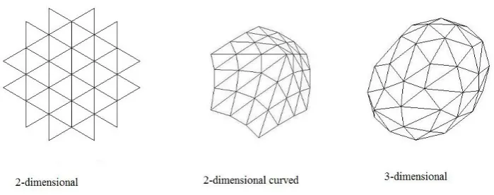
With CDT, the basic space elements are n-dimensional simplexes (e.g., triangles, tetrahedrons; see 288
Fig.1). In contrast to CDT, the proposed causal model of curved discrete spacetime considers only 289
3-dimensional space elements, i.e., tetrahedrons. The time dimension is treated separately within the 290
causal model. In addition, the elementary units that represent the total space are not (as with CDT) the 291
n-dimensional simplexes, but only the space points together with their connections to neighboring 292
space points The reason for this simplification was that it was not possible to build up a larger space 293
object by the continuous addition of uniform regular tetrahedrons and (2) the uniformness of the 294
tetrahedrons is obsolete with the proposed model (see Section 4). Whether the space points together 295
with the connections establish specific 2-dimensional surface areas (e.g., triangles) and 3-dimensional 296
solids (e.g., tetrahedrons) is initially left open. 297
Definition 1. Space := { spacepoint ...}; 298
spacepoint := {ψ,dilation f actor,connections }; 299
connections := { connection1, ...,connectionn}; 300
Figure 1.Elements of spacetime of Causal Dynamical Triangulation.
ψis the physical content that is directly associated with the space. These are the fields residing 302
in space. As with spin networks, spin foam networks, and causal dynamical triangulation, each 303
space point is connected with a number of other space points via "connections" (i.e., edges in CDT). A 304
connection carries the information about the connected neighbor space point, the connection direction, 305
and the propagation gradient of the curvature changes (see Section 4). 306
All the information associated with the space point is local to the space point (i.e., no globally 307
defined position or direction specification). This supports the background independence of the 308
spacetime model. 309
To enable the determination of the spatial distance between two space points, some information 310
about the distance between neighbor space points is required. This could be provided, for example, 311
in form of position coordinates (Provision of space point coordinates would violate background 312
independence). or by the specification of the lengths of connections between the neighbor space points. 313
In support of a causal model of the movement of objects in curved space, for the proposed model of 314
spacetime dynamics, it is defined that 315
Proposition 3. The length of the connections between space points is a constant; 316
Lconnection =c·SUT I. 317
2The overall distance between two space points within the curved space is then obtained by 318
multiplyingLconnection by the number of space pointskpon the geodesic path from space point-1 to 319
space point-2. Length dilation within a gravitational potential as assumed by Proposition 1 in Section 320
3.1, is realized by the appropriate arrangement of the space points within space (see Section 4). 321
Proposition 3 is, first of all, a physical statement, although it has consequences for the space 322
geometry. The physical statement is: 323
The (spatial) distance that light moves during a state update time interval (SUTI) is equal to the distance 324
between two connected neighbor space points, which is equal to the distance by which space expands during a 325
SUTI. 326
The geometry of the emerged space (e.g., whether an Euclidean space or a Schwarzschild metric 327
emerges) depends on the space expansion algorithm. With the proposed model of spacetime dynamics 328
the resulting geometry depends on the ratio by which the number of space points grow at a single 329
expansion step (see Section 4.1). 330
3.3. The representation of space(-time) curvature 331
Space curvature is a major ingredient of GRT. In GRT, specifically in Einstein’s equation 332
Gαβ= 8πG c4 Tαβ,
333
space curvature is expressed by the curvature tensorGαβ. Thus, the simplest solution would be to say 334
that a space-curvature component is assigned to the space point and that this curvature specification 335
provides the same information as the curvature tensor of GRT. However, some adaptations appear 336
reasonable. In Section 3.2 above, the space component of the system state is specified as consisting 337
of a set of space points, and, at the next level of detail, a space point is specified as consisting of 338
dilationfactor, connections, and the space contentψ. 339
spacepoint := {ψ,dilation f actor,connections}; 340
The dilationfactor supports the generation of the space curvature with the propagation of space 341
changes (including the emergence of space). Once the space has emerged, the space(-time) curvature 342
is represented by (1) the distribution and density of the space points and (2) the (spatial) distances 343
between neighboring space points. Proposition 3 (above) states that the length of the connections 344
between space points, i.e., the distances between neighboring space points, is a constant. Thus, the 345
main parameter that determines the space curvature is the density distribution of the space points. 346
The density distribution of space points is realized by the appropriate arrangement of the space points 347
within space. 348
As described in Section 3.1, Proposition 2, the the clock rate dilation (i.e., the time-related 349
component of the GRT curvature) is a consequence of the length dilations. This means that the 350
information which specifies the length dilations implies the time-related component of the GRT 351
curvature. 352
4. Space(-time) dynamics
353
The dynamics of spacetime is triggered by the minimal sources, called "quantum objects". With 354
each update cycle of the system state a new space change action starts at each quantum object. The 355
space changes propagate from the quantum objects through the whole space in steps according to the 356
update cycles of the physics engine. In support of alocalcausal model, with each update cycle, the 357
space changes propagate only to (part of) the neighboring space points. The propagating space changes 358
always have definite directions at each space point, from the "in-connections" to the "out-connections" 359
of the space point. The out-connections of space point sp, at a given update cycle i, are in-connections 360
of some neighbor space points of sp with the subsequent update cycle i+1. 361
The directions of space changes, i.e., the identification of in/out-connections, are determined 362
by the∆curvatureattribute of the space point connections. For a given space point, only part of 363
the connections can be in-connections, which meansconnection.∆curvature > 0. The remaining 364
connections of the space point are out-connections. 365
The overall process of space change propagation is specified as 366
Specification 1. spaceprogression():={ 367
FOR ( all space pointsspi){ 368
IF ( inconnections(spi) { 369
propagateOUT(spi); 370
} } 371
} 372
4.1. The emergence of space from a single source 373
The space that emerges from a single source represents a Schwarzschild metric. In the causal 374
model, the large-scale space object emerges by the successive addition of surface layers to the initial 375
377
SSspaceemergence( source ) ::= { 378
spaceobject←source; 379
DO UNT IL(nonContinueState(S)){ 380
spaceobject←extendbynextlayer(spaceobject); 381
} 382
} 383
For the refinement of the above space emergence process, answers to the following questions have to 384
be provided: 385
1. What are the elementary units of space? 386
2. How does the initial space object look like? 387
3. What is the detailed algorithm forextendbynextlayer(spaceobject)? 388
4.1.1. The elementary units of space 389
The elementary structure of space, including the elementary units of space, have already been 390
described in Section 3.2. In the proposed model, the elementary units of space are the space points 391
together with their connections to neighbor space points (see Definition 1). The number of connections 392
(and thus the number of neighbor space points) of a given space point must be large enough to span 393
the complete three-dimensional space. It should be small enough to enable a moderate growth of the 394
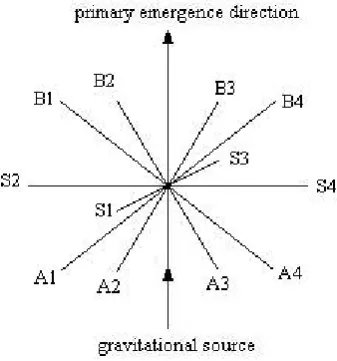
number of space points with the chosen algorithm of the space emergence process. In the model, a 395
typical space point has 14 connections (see Fig.2): 396
• source connection: one connection towards the source of the emerging space, 397
• target connection: one connection in the primary emerging direction, 398
• surface connections: four connections in the plane that is perpendicular to the source connection 399
(S1, S2, S3, S4 in Fig.2), 400
• four connections in between the source connection and the surface connections (A1, A2, A3, A4 401
in Fig.2), 402
• four connections in between the target connection and the surface connections (B1, B2, B3, B4 in 403
Fig.2). 404
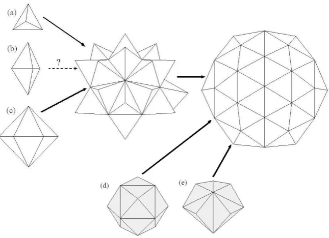
Figure 3.Alternative initial space elements.
4.1.2. The initial space object 405
There are several alternatives for the initial space object from where the emergence of space and 406
the propagation of gravitational space dynamics may start. Fig. 3shows a number of alternatives 407
investigated by the author. The simplest solution would be to have the space emergence process, 408
starting from a single tetrahedron (case (a) in Fig. 3) or a double-tetrahedron (case (b) in Fig. 3) . 409
However, more symmetrical initial space objects, such as case (c) or case (d) enable the early emergence 410
of a symmetrical larger space object through simple space extension algorithms. For the present model 411
of spacetime dynamics the initial space object is a single space point surrounded by 14 neighbor space 412
points and the respective connections. The 14 neighbor space points, together with the interconnections 413
among them represent a spherical surface - the initial surface from where the space emergence starts 414
(case (d) in Fig.3). 415
4.1.3. The space expansion algorithm-extendbynextlayer(spaceobject)
416
As described above, space emergence from a single source is a continuous process where each 417
system state update cycle of the causal model adds another layer of space to the existing space object. 418
This means, with each expansion stepstia numberkpiof new space points is generated. The new space 419
points are interconnected with their respective neighbor space point, formingktisurface triangles. 420
Various kinds of space expansion algorithms are possible. The key differentiating parameters for 421
the alternative space expansion algorithms are the growth factor gp of the number of surface space 422
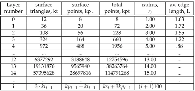
points (i.e.,kpi=gp·kpi−1) and the related growth factor gt of the number of surface triangles (i.e., 423
kti =gt·kti−1). Table 1 shows the major parameters for an example space emergence algorithm that 424
starts with an initial space object with 12 surface triangles (case (c) in Fig. 3). The surface growth 425
factorgt=3, i.e.,kti =3·kti−1. The number of surface space points increases by the number of surface 426
triangles,kpi=kpi−1+kti−1. 427
Further parameters shown in Table 1 are the total number of space points, the radiusriof the surface 428
and the average edge length, L of the surface triangles. The average edge length, L is the length 429
measured by the author’s computer simulations and these computer simulations and the length 430
measurements assumeEuclidean space. However,the space emergence process of the model of spacetime 431
Table 1.Layers of space expansion, constant surface∆r=1.0
Layer surface surface total radius, av. edge
number triangles, kt points, kp . points, kpt ri length, L
0 12 8 8 1.00 1.63
1 36 20 72 2.00 1.72
2 108 56 228 3.00 1.55
3 324 164 660 4.00 1.22
4 972 488 1956 5.00 .88
... ... ... ... ... . ...
12 6377292 3188648 12754596 13.00 ...
13 19131876 9565940 38263764 14.00 ...
14 57395628 28697816 114791268 15.00 ...
... ... ... ... ... ...
i 3·kti−1 kpi−1+kti−1 ksi+3kpi−1 (i+1)100
accordance with the Propositions 1, 2 and 3. Especially, Proposition 3 says thatLconnectionis constant. 433
With the example shown in Table 1,Lconnection = ∆r = 1.0. This means that the circumference of a 434
surface, if curved space andLconnection = 1.0 is assumed, depends solely on the number of surface 435
space points,kpi. The number of surface space points,kpifor a surfaceSiis determined by the space 436
expansion algorithm. For the proposed model of spacetime dynamics, a curved space with length 437
dilations according toF1at the surfaces (see Eq. 2) has to emerge. This can only be achieved with 438
a decreasing growth factor gp. The space expansion algorithms that have been investigated by the 439
author showed that with the proposed model, GRT compatible space expansion algorithms are feasible. 440
However, unless the algorithm gets unnaturally complex, occasional inhomogeneities seem to be 441
unavoidable. In particular at the very small scale, i.e., near the minimal gravitational sources, it 442
appears to be difficult or impossible to preserve the GRT compatible behaviour. The surrender of 443
perfect GRT compatibility at the very small scale may avoid singularities that occur with the differential 444
equations of GRT. 445
4.2. The propagation of space changes caused by multiple sources 446
The assumption that space changes start at the minimal sources implies that the aggregation of 447
space changes from many sources is the normal case. The model of the propagation of space changes 448
that are caused by multiple sources is based on the single-source propagation (Section 4.1). The 449
aggregation of the single-source propagations has to be accomplished by a local causal process, i.e., 450
by a series of aggregations of neighboring space changes. Only long range, this dynamical process, 451
can achieve overall gravitational space changes (i.e., curvature changes) that are compatible with the 452
predictions of GRT and Newtonian dynamics. 453
To simplify the description, in this article, "multiple sources" is initially equated to "two sources". 454
In simple cases, the treatment of many sources can be performed by a series of two source propagation 455
processes. 456
For the overall two-source propagation process, three phases can be distinguished: 457
• Phase-1, the phase where the changes from the two sources propagate independently. 458
• Phase-2, the phase where the changes start to overlap and therefore have to be aggregated. 459
• Phase-3, the phase where the aggregated changes propagate like single source changes. 460
Fig.4shows an example snapshot in two dimensions, with the areas that are covered by phase-1 and 461
phase-3 roughly indicated. Notice that the 2-dimensional representation in Fig.4is a simplification 462
which is misleading with certain more detailed considerations. 463
A major assumption of the proposed model is that the propagation that occurs at a space point 464
Figure 4.Propagation of space changes caused by 2 sources.
in-direction is the vector sum of the multiple in-connections. The overall out-direction is distributed 466
over the multiple out-connections. 467
4.2.1. Phase-1: 468
The propagation of space changes prior to the points where the changes meet is exactly the single 469
source propagation described in Section 4.1. 470
4.2.2. Phase-2: 471
When the space changes originating from (two) different sources meet at space point sp, the 472
changes that arrive from n space point connections ( n≥2 ) are summarized into a single out-vector. 473
The out-vector is then distributed to the out-connections (see Fig. 4, the magnifying glass area). 474
If there are no out-connections left – i.e., if all connections of sp are in-connections – the weakest 475
in-connection(s) are taken as out-connection(s). 476
4.2.3. Phase-3: 477
After the changes from the multiple sources are summed up, the further common propagation 478
of the space changes continues like the single-source propagation (Section 4.1). As a special case, 479
the phase-3 propagation may collide with phase-1 propagation from one of the two sources. With 480
the proposed model of spacetime dynamics, the collision of space changes is handled like a phase-2 481
propagation, described above. 482
Compatibility with classical, i.e., Newtonian dynamics evolves during phase-3. The compatibility 483
with classical dynamics is reflected in mainly the following items: 484
1. It is valid to assume an aggregated massMaggrthat represents the aggregation of the masses of 485
2. It is valid and possible to identify a position in space whereMaggris assumed to be located. The 487
position is usually called the "center of mass". 488
3. The (single) aggregated massMaggris the sum of the masses of the sources of the space changes. 489
Maggr =M1+...+Mn. 490
Only when the propagation of space changes reaches a certain distance r from the center of mass 491
that the aggregated massMaggr(r)can be equated to the sum of the masses of the sources. 492
4.2.4. Aggregation of space dynamics from n2 sources 493
The above-described model of the space dynamics aggregation from two sources, with the three 494
aggregation phases shows that compatibility with classical dynamics will only evolve at the end of 495
phase-3. Prior to that stage, inhomogeneities, i.e., areas where only a subset of the gravitational source 496
participates in the aggregation, will occur (and will not disappear during the continued propagation of 497
space changes). If the aggregation of space dynamics applies to n2sources, further inhomogeneities 498
may exist, depending on the distribution of the sources within the space. If the distribution of the 499
sources establishes gravitational sub-clusters such as solid bodies, planets or stars, where it is possible 500
to assign an aggregated massMaggrand a center of mass, the sub-clusters may represent a gravitational 501
source at the next higher level. 502
5. Applications of the model of spacetime dynamics to quantum field theory
503
In Sections 3 and 4, a causal model of the dynamics of spacetime has been described. According 504
to the model, spacetime changes (i.e. the gravitational field) continuously propagate from the minimal 505
sources, called quantum objects. In quantum field theory (QFT), the quantum objects are also the 506
sources of additional dynamical processes. Quantum objects are the sources of virtual particle 507
fluctuations. The movement of quantum objects through space, is described in terms of paths that 508
constitute the wave function. Also, particle scattering in QFT is described in terms of paths for 509
virtual particles that lead to a range of probability amplitudes for different possible scattering results. 510
Considering the various cases of the dynamics in QFT, the question arises on how QFT (virtual particle) 511
paths relate to the model of spacetime dynamics described in the preceding sections. As with the 512
general subject, the question can be asked in two parts: 513
1. How do the dynamics of quantum fields (including quantum objects) relate to the elementary 514
structure of spacetime described in Section 3? 515
2. How do the dynamics of quantum fields (including quantum objects) relate to the model of the 516
dynamics of spacetime described in Section 4? 517
Question 1 requests a detailed answer in order to demonstrate that the model of spacetime dynamics 518
can also be applied to the dynamics of quantum fields and quantum objects. The details are straight 519
forward, yet non-trivial. The answer to question 2 is less direct. Integrating quantum field dynamics 520
and spacetime dynamics at different degrees are imaginable, ranging from minimal integration (i.e., 521
adaptation to the proposed spacetime structure only) to maximal integration (i.e. a combined model 522
for both subjects as for example quantum gravity aims for). In Section 5.2 the model proposed by the 523
author is described. 524
5.1. Mapping quantum fields and quantum objects to the elementary structure of spacetime 525
The task is to map the parameters and components that constitute a quantum field or a quantum 526
object to the parameters and components of the spacetime as described in Section 3. In Section 3.1, 527
the integrated view of spacetime (as assumed in standard GRT) is described as being disturbed by 528
the strict separation of space and time implied by thecausalmodel. This may be considered as too 529
restrictive for a GRT-compatible model of spacetime to be applied to QFT. However, starting with a 530
topology where space and time are separated intoΣ×RwhereΣis a three-dimensional manifold and 531
quantum gravity). It leads to the so-called "Hamiltonian formulation of general relativity" (see [16]). 533
As with the model of spacetime dynamics described in this article, the integrated view of spacetime is 534
restored by processes that relate the spatial changes to the progression of time (e.g., by a causal model). 535
In Section 3.2, Definition 1, space is defined as consisting of interconnected space points and a 536
space point is defined as 537
spacepoint := {ψ,dilation f actor,connections}. 538
Here, fields are represented by the componentψ. (Whetherψrefers to a single type of field or to 539
possibly multiple field types is here left open.) In [3], quantum objects are defined as composite objects 540
consisting of 1 to n particles. 541
Definition 2. quantumobject:={ 542
globalquantumobjectattributes; 543
particle1, 544
... 545
particlen; 546
} 547
The particle encompasses a set of spacepoints andglobal particleattributes: 548
Definition 3. particle:={ 549
global particleattributes; 550
spacepoint1, 551
... 552
spacepointk; 553
} 554
Examples of global attributes ( globalquantumobjectattributes and globalparticleattributes ) are 555
mass, charge, spin, etc. With the specification of alocalcausal model at a specific level of detail, the 556
inclusion of the global attributes may disturb the provision of alocalcausal model. Therefore, in a 557
detailed local causal model, the global attributes may have to be supported by aggregation processes 558
and/or collective behaviour processes (see Section 5.3 Collective behaviour). 559
5.2. Mapping of the dynamics of quantum fields and quantum objects to the dynamics of spacetime 560
The model that is roughly described as follows is based on two types of work: 561
1. Loop quantum gravity [16] and its descendants comprising spin networks (see [17]), spin foam 562
(see [18]), and causal dynamical triangulation [4]. 563
The coupling of the dynamics of space (e.g., the propagation of space changes) with the dynamics 564
of quantum fields and particles is an idea that has already been pursued with causal fermion 565
systems (see [20]). 566
2. In [1] and [3] a causal model of QT/QFT is proposed where the physics of QT/QFT is confined 567
in "quantum objects". The refinement and an improved foundation of the model described in [1] 568
and [3] was determined to require a causal model of spacetime dynamics. The causal model of 569
spacetime dynamics described in Sections 3 and 4 has been developed as an attempt to fulfill this 570
requirement. 571
5.2.1. The movement of objects within space 572
According to GRT, the movement of objects within space follows the geodesics of the space. 573
This means, two parameters determine the path of the object: (1) the objects momentum and (2) the 574
With the model of spacetime dynamics, especially when applied to quantum theory, the 576
GRT-based model of object movement has to be adjusted and refined for two aspects: (1) the term 577
geodesics must be redefined for discrete granular paths, and (2) the momentum of quantum objects in 578
general does not have a single definite value, but a range of (possible) values. Regarding these two 579
aspects resulted in the following model for the movement of objects within space. 580
• The moving object is represented by the space contentψof a set of space points (see Definition 1). 581
• Part ofψis the momentum vector component p. 582
• When the propagation process reaches a space point sp, the momentum vectors from the 583
in-connections of sp are summarized to a single consolidated momentum vector. 584
• The consolidated momentum vector is then distributed to the out-connections. 585
• The distribution is such that the out-connection(s), which matches best the direction of the 586
consolidated momentum vector, obtains the largest part of the consolidated vector. 587
Given the aforementioned schema, the following types of object movements may be distinguished: 588
1. Classical straight forward movement following a single definite geodesic, 589
2. Quantum movement with a network of paths and with different probability amplitudes, 590
3. Loops 591
(a) Classical loops according to a geodesic that represents a loop (examples: planets and 592
satellites), 593
(b) Quantum loops: Loops resulting from quantum objects and constituting quantum objects. 594
Quantum movements and quantum loops are further described in the following. 595
5.2.2. Quantum movement 596
In Section 4, the dynamics of spacetime is described as involving the summation of the 597
in-connections of a space point followed by the distribution of the aggregated effect to the multiple 598
out-connections. A similar operation is also known with the operator equations of QFT (see, for 599
example [21]). Two virtual particles may join and annihilate each other to create a single new virtual 600
particle of a specific type; or vice versa, a single virtual particle may be annihilated resulting in 601
the creation of two new virtual particles of specific types. The graphical representation of the 602
possible annihilate/create (or join/split) operations is given by Feynman diagrams. In quantum 603
electrodynamics (QED), the operator equation for the creation and annihilation of the field has the 604
form (see [21]): 605
HW(x) =−eN{(ψ¯++ψ¯−)(6A++6 A−)(ψ+−ψ−)}x 606
whereψ+,ψ−, ¯ψ+, ¯ψ−,6 A+,6 A− are the creation and annihilation operators for electron, positron 607
and photon. This leads to the eight fundamental Feynman diagrams shown in Fig.5. The operator
Figure 5.Fundamental Feynman diagrams of quantum electrodynamics.
combination of QFT (normally) applies to three operations (two creates and one annihilate or one 609
create and two annihilate). For a mapping of the QFT processes to the model of spacetime dynamics, 610
the QFT operations have to be mapped to the n in/out connections of the space point. A typical
Figure 6.Possible QED connections of a space point.
611
space point has n = 14 connections. This enables the use of various strategies (i.e. algorithms) for 612
the mapping of the three lines of a fundamental Feynman diagram to the 14 space point connections. 613
For the application of the model of spacetime dynamics to quantum fields, the overall strategy is the 614
preservation of the number of fermion in-connections and fermion-out connections and the allowance 615
of additional boson connections. This enables the types of QED space point connections shown in 616
Fig.6. (For practical purposes only part of the boson connections are shown in Fig.6). The cases that 617
correspond to the QED first order diagrams shown in Fig.5are the cases (1) to (3) in Fig.6. Case (4) 618
and case (5) support an increased diversity of the possible fermion and boson paths. 619
Notice that the mapping of the QFT operations to the in/out connections of the space points is 620
part of the dynamical QFT processes (it is not a static mapping). 621
The utilization of the complete set of in/out connections for the join/split operation on (virtual) 622
particle paths delivers the equivalent to the superposition of paths which in QFT is expressed by the 623
path integral. In standard QFT (see [19] ), the path integral is written as 624
K(b,a) =Rabe(i/¯h)S[b,a]Dx(t). 625
The discreteness of the model parameters (space, time and paths) may results in significant 626
incompatibilities at the very small scale. The discreteness of the model parameters in conjunction 627
with thelocal causalmodel eliminates the need for renormalization (if a suitable algorithm for the 628
assignment of in/out connections is applied). 629
5.2.3. Quantum loops 630
In terms of a causal model, a physical object moves into a loop, if two conditions are satisfied: 631
1. The object moves in a spatial environment that enablesgeodesic loops. 632
2. The object has reached arecurrence state, i.e., a state such that the causal progression of the object 633
may lead to a recurrence of this object state. 634
Geodesic loops can occur only if space has a specific curvature. The simplest example of space 635
curvature that enables geodesic loops are the spherical surfaces that develop with the emergence 636
of space caused by one or multiple sources (see Sections 3 and 4 and Fig. 7). With the model of 637
Figure 7.Surface of space that enables geodesic loops.
spherical surfaces. The spherical surfaces occur already around the minimal sources, i.e., the quantum 639
objects. As described above (see Quantum movement), in contrast to GRT, where the geodesics are 640
single lines, in the model proposed, the geodesic consists of a network of paths with splits and joins 641
at each space point according to the rules and diagrams of QFT. This holds true also for the geodesic 642
loops (see Fig.8). Because of the large number n of in/out connection (n>3,n∼14) , there may be 643
paths of the network that do not end up in the loop. In general, there will be open ends (see Fig.8).
Figure 8.A quantum loop containing a network of paths.
644
In the quantum loop shown in Fig. 8, the in/out connections are labeled by specific symbols. 645
In Fig. 8the labels (and thus the paths) refer to (virtual) particle types of QED (γ,e−, e+). This 646
emphasizes the close relationship between the quantum loop network and Feynman diagrams. An 647
alternative labeling of the paths, and thus an alternative interpretation of the quantum loop, would be 648
to show the similarity with spin networks. With spin networks, the connections (i.e., line segments) 649
within the network are attributed by spin numbers (with the original introduction by R.Penrose [17]) 650
or the dimension of the parallel transport matrix (see [16]). Similar to spin networks, the quantum 651
loop network defines the possible paths of state transitions including possible final result state (i.e., the 652
recurrence state). If an extra (logical) dimension is added to the quantum loop network (or to the spin 653
network) to show the complete multitude of possible networks that support a specific recurrence state, 654
5.3. Collective behaviour 656
One of the objectives of the causal model presented in this article is that the model should be a 657
localcausal model. The target space-point-locality is damaged by the inclusion of composite quantum 658
objects with object-global attributes (e.g. mass and spin) and instantaneous processes (e.g., the collapse 659
of the wave function and entanglement), if it is not possible to break down the formation of the 660
composite objects and the related non-local effects to space-point-local state transitions. In the causal 661
model of QT/QFT described in [2], the non-local effects are explained by the collective behaviour of 662
spacetime elements. Based on the causal model of spacetime dynamics described in Sections 3 and 4 663
and the concept of the quantum loops, the model described in [2] can now be refined as follows. 664
The formation of (semi-) stable quantum objects (elementary as well as composite quantum 665
objects) is a collective behaviour process in form of a quantum loop that runs within the (small) area of 666
curved space around the components of the quantum object. 667
As the described collective behaviour process represents a model for the emergence of quantum 668
objects and the related quantum-object-global attributes, the disturbance of this collective behaviour 669
process provides a possible model for the instantaneous non-local QT/QFT processes such as particle 670
decay, the collapse of the wave function, and decoherence. The model which describes the emergence 671
of a quantum object as a collective behaviour process has many similarities with G. Groessing’s 672
proposal to explain the emergence of a quantum system as a self-organization process (see [22]). 673
6. Applications of the model of spacetime dynamics to cosmological dynamics
674
In addition to enabling alternative interpretations and models of QFT in curved spacetime 675
(the topic of Section 5), the proposed model of spacetime dynamics also leads to (possible) new 676
interpretations and models of cosmological dynamics. The main features of the model of spacetime 677
dynamics that enable/demand new interpretations are (1) gravitational length dilations and (2) the 678
non-smooth aggregation of spacetime dynamics. 679
6.1. Gravitational length dilations 680
Propositions 1 and 2 in Section 3.1 state that wherever GRT predicts a time dilation, this time 681
dilation is accompanied by a length dilation (in fact, the propositions say that the length dilation is 682
the primary effect, and that the clock rate dilation is a consequence of the length dilation). Applied to 683
cosmological dynamics, this means that the lengths of the orbits of cosmological objects (e.g. stars, 684
planets, moons) orbiting a gravitational source are dilated by a factor ofF1= q
1−2GMc2r (see Eq.2).
685
Since the radius r is only dilated by a factorFr <F1, this means that, contrary to Euclidean geometry, 686
the circumference C of an orbit around a gravitational source is greater than 2πr. The dilation of the 687
circumference is an effect which cannot be directly observed by an observer such as an astronomer. 688
In the projection of the orbit to a picture in Euclidean geometry, the relation between the observed 689
radiusro and the observed circumferenceCo is stillCo = 2πro. The orbital length dilation can be 690
observed only indirectly, by examining the dynamics of objects orbiting around a gravitational source. 691
For example, the velocity of objects orbiting a gravitational source will show deviations from the 692
laws of Newtonian dynamics. The most famous examples of unexpected deviations from Newtonian 693
dynamics in cosmological observations are the "flat galaxy rotational curves", for which gravitational 694
length dilations offer a possible explanation (see below). 695
In Section 3.5, Proposition 2 states that in the proposed model of spacetime dynamics, clock rate 696
dilation is considered a secondary effect caused by the primary effect, the length dilation due to space 697
curvature, i.e., due to the gravitational field. According to Section 3.5, the lengths (and, as a secondary 698
effect, also the clock rates) around a gravitational source are dilated by the factor 699
F1= q
1−2GM c2r .
This means, that if at a spacepoint near the gravitational source, at radius r1, the dilation factor is F1=
q
1−2GM
factor gets closer to its maximal value, 1. If, for two neighboring spacepoints at equal radius r=r1, the non-dilated distance between them isdN, the dilated distanceddisdd=dN·F1(r1).3
(The subscript N stands for "Newtonian" or "non-dilated", d stands for "dilated", and o stands for "observed")
For larger distances, the overall dilated path length following the spacepointssp1, ...,spkis
pld(sp1, ...,spk) = k−1
∑
i=1l.connection(spi,spi+1)·F1(r1) (3)
For paths on a (Schwarzschild metric) circumsphere, i.e., with constant radius r, this can be simplified 700
to 701
circumspherepld(sp1, ...,spk) =F1(r)·pathN(sp1, ...,spk) by settingpathN(sp1, ...,spk) =∑ik−=11l.connection(spi,spi+1).
In Eq. (4), the dilated path length is obtained by multiplying the "non-dilated" path length by the factor F1, leaving aside that alwaysF1≤1. In order to avoid misinterpretations and use a more meaningful base for the dilation factor, the dilation factorF2is introduced such that
circumspherepld(sp1, ...,spk) =F2·pathN(sp1, ...,spk) (4) andF2is defined asF2(r) =F1(r)/F1(r0), with r0 being the minimal radius (e.g., r0 = 1). This ensures 702
thatF2is alwaysF2≥1. 703
In radial direction, matters are more complicated because the factorF2varies with increasing radius. Let us define that instead of the factorF2, the dilated length in radial direction is dependent on a factorF3
radial pld(sp1, ...,spk) =F3·pathN(sp1, ...,spk). (5) The difference between F3andF2depends on several parameters. (For the special case of galactic 704
rotational curves, the parameters are described in Section 6.3.) In general,F3<F2. This means that for 705
a sphere with radiusrdaround a gravitational source the dilated circumferencecd6=2πrd. 706
6.1.1. The observation of space distortion by a distant observer 707
For the analysis of the implications of the gravitational length dilations for cosmological models, 708
it is important to analyze the extent to which the length dilations can be observed by a distant observer, 709
such as an astronomer. The (3-dimensional) space distortion due to non-uniform length scale (like 710
other space curvature) can hardly be directly observed. It can be indirectly observed, by observing 711
an object’s movement within a strong gravitational field or by observing the large-scale results of 712
dynamical space(-time) processes. Astronomers who observe the cosmos typically obtain projections of 713
3-dimensional curved space configurations to 2-dimensional images. Assuming that the Z-axis points 714
to the observer, the projections apply to the (X,Y)-plane. The length dilations in radial directions (from 715
the gravitational source) also appear in the projections; that is, they can be observed. As described 716
above, lengths in radial directions are dilated by the factorF3. 717
The dilation of lengths that are not purely in radial direction will also appear in the observations, 718
but only to the extent of the radial direction dilation. For example, according to the description given 719
above, the orbit around a gravitational source is dilated by the factorF2(F3≤F2). The distant observer, 720
however, will see the length of the orbit asrd·2π, with the dilated radiusrd= non-dilated-radius·F3. 721
Furthermore, the length projections for an area of the cosmos (i.e., observations) must be seen in 722
relation to the space distortions in the surrounding space. 723
6.2. Non-smooth aggregation of spacetime dynamics 724
In cosmology, it is well known that the strength of the gravitational field within a (dense) 725
gravitational object increases in a different manner with increasing distance from the centre of mass 726
than is the case outside the object. Section 4.2 explains that the process of aggregation of spacetime 727
curvature changes resulting from several sources may be even more complex than assumed in the 728
standard models. This may affect various aspects of the cosmological models. 729
730
The features of the proposed model of spacetime dynamics described above may have implications for 731
many aspects of the present standard cosmological model. On the positive side, these features also 732
offer opportunities for new explanations and interpretations in areas of cosmology that are not yet 733
sufficiently understood. The major areas identified by the author in which the application of the model 734
of spacetime dynamics may result in new explanations of cosmological observations are the following: 735
6.3. Flat galaxy rotational curves and dark matter 736
The existence of "dark matter" has been proposed as a possible explanation of the observed flat 737
galaxy rotational curves, while an alternative explanation known as modified Newtonian dynamics 738
(MOND) has also been proposed. Two further proposed theories explain the flat rotational curves by 739
the existence of a new force: (i) a so-called entropic force (see [23]) or (ii) a so-called gravo-inductive 740
field (see [24]). 741
Gravitational length dilation (see above) may provide yet another possible explanation for the flat 742
galaxy rotational curves, in which the length and clock rate dilation (i.e. time dilation) yield a velocity 743
larger than that deduced from the observed rotational curves. In simpler terms, the rotational curves 744
are observed due to the spacetime curvature, in which the orbit has a larger length dilation factor than 745
the radius.
Figure 9.Velocities in galaxy rotational curves.
746
Table 2.Galaxy rotational curves
dilation circulation circunference radius velocity
cases factors time, t c r v
w/o dilation 1 tN cN=2πrN rN vN=cN/tN
dilated F2,F3 td=tNF2 cd=cNF2 rd=rNF3 vd=vN
observed - to=tN co=2πro ro=rd=rNF3 vo=co/to
Example:
w/o dilation 1 100 628 100 6.28
dilated 1.1, 1.05 110 690.8 105 6.28
observed - to=tN =100 co=cN=660 105 6.6
phases are distinguished with respect to the velocity v of circular orbits (see Fig.9).4In phase-1, when the star is within (or close to) the "bulge" that surrounds the center of the galaxy, the velocity according to Newtonian dynamics is
v(r) = r
GM(r)
r . (6)
G is the gravitation constant, r the radius, and M(r) the mass, which is dependent on the radius. Resolving the dependency of the mass on the radius by application of the density lawM(r) =ρ0V (see [27] ), results in v(r) being proportianal to r:
v(r)∼r. (7)
When the distance from the bulge is sufficiently large phase-2 applies where the velocity is expected to be
v(r)∼
r
1
r. (8)
For phase-1, the observations are in agreement with the expectation. Phase-2 presents a problem. 747
Instead of the decreasing velocity (Fig.9,vN), according to Eq. (9), a flat rotational curve is observed 748
(Fig.9,vo), i.e., the velocity observed is greater than expected. 749
In addition to the dark matter theory and the MOND theory, the length dilation assumed with 750
the proposed causal model of spacetime dynamics may provide another explanation for the flat galaxy 751
rotational curves. The explanation concerns, first of all, the differences in the length dilation of the 752
circumference of the rotational curve and the length dilation of the radius. This difference is the 753
difference between the factorsF3andF2, described in Section 6.1. The difference betweenF3andF2 754
causes differences between the observed values and the real values of the physical parameters as 755
described in Section 6.1.1. 756
In the context of galactic rotational curves, for the calculation of the value ofF3, the following 757
points have to be taken into account: 758
1. In contrast toF2in Eq. (5),F3in Eq. (6) is the mean value for a path with varying radius r. 759
2. The complete range of radius to be considered includes the phase-1 part, the phase-2 part, and 760
the part between phase-1 and phase-2. In addition to the uncertainty as to where exactly phase-1 761
ends and where exactly phase-2 starts, the following points are difficult to quantify: 762
3. During phase-1, not only doesF2(the basis for determiningF3) vary with r, but as indicated in 763
Eq. (7) the (effective) mass M(r) also increases with increasing radius. 764
4. As described in Section 4.2, the author questions the general applicability of the density law 765
M(r) =ρ0Vfor the determination of M(r) for the complete phase-1. 766