Rainfall-runoff modeling of the Nyando River basin for flood mitigation

,

\

RAINFALL~RUNOFF

MODELING OF THE NYANDO IUVE

R BAS

I

-N

,

FOR FLOOD MITIGATION

I;

By

ELLYOKE

AJIGOH

A THESIS SUBMITTED IN PARTIAL FULFILLMENT OF THE REQUIREMENTS FOR

THE AWARD OF THE DEGREE OF MASTER OF SCIENCE IN HYDROLOGY AND

WATER RESOURCES IN THE SCHOOL OF PURE AND APPLIED SCIENCES OF

KENYAITA UNIVERSITY

Ajigoh, O. -~~~ Rainjall-runnoff modeling of the

1111111111111111

DECLARATION

This thesis is my original work and has not been presented for a degree in any other University or any other award.

Signature

c::..~~~.

Okewe Ajigoh

Date

We confirm that this thesis has been submitted with our approval as university supervisors:

Signature ... ~ ..

.

.

2~I

..

p..«.I..

~.e

.

1.

Dr. Christopher

IT

Date

Signa

& ~ ~

.

..

2.?:

:

f.

.

o.

..

~

..

fQ

.

~

.

Dr. Joy A. Obando

GEOGRAPHY DEPARTMENT KENYA

ITA

DEDICATION

ACKNOWLEDGEMENT

I am especially grateful to my supervisors Dr. C.M.Ondieki and Dr.

l.A

.

Obando

For their critical comments and contributions during my thesis work

_

Special thanks to the various institutions and organizations that provided data especially

ministry of water development and Irrigation for stream flow data and the Meteorological

department for the rainfall data

'

To the poly leT staff, thanks for providing us with the unlimited time on the internet. Special

thanks to the staff of

Kenya polytechnic GIS laboratory. In particular Mr. Lusichi who was

always ready to assist with Gis tools

'

Last but not least ,thanks to my colleagues in 2004 class for the masters

of science in

Hydrology and water resources namely; Mr. Julius Wanyonyi(posthumously),Mr. Ronald

sungu, Mr. John K. Mwangi and my research college Mr. Muli

L

TABLE OF CONTENTS

Title .i

Declaration .ii

Dedication .iii

Acknowledgements .iv

Table of contents v

List of tables xi

List of figures xii

Abbreviations and acronyms xiv

Abstract, , xv

CHAPTER ONE:

INTRODUCTION

1.Background 1

1.1Area of study 2

1.2 Relief and Drainage 2

1.3 Climate 4

1.4 Geology and Soils 4

1.5 Problem .statement. 6

1.6 Justification 8

1.7 Main objective 8

1.8 Specific objective .9

1.9 Research questions

:

:·

.

~

.9

1.10 Significance of study 9

CHAPTER

T

WO: LITERATURE REVIEW

2.Introduction '" 11

2.1 Flood generation processes 11

2.2 Flood: the underlying factors 14

2.3 Models 19

2.3.1 Categorization of mathematical models 20

2.3.2 HEC-lIMS , 22

2.3.3 Constituents of a model. 23 I

CHAPTER THREE: METHODOLOGY

_

3 Introduction 25

3.1 Data Acquisition and processing 25

3.2 Data Analysis 29

3.2.1 Stream Flow 29

3.2.2 Rainfall 30

3.2.3 Correlation and Regression 31

3.3 Frequency Analysis 32

3.3.1 Fitting a distribution 35

3.3.2 Plotting position 36

3.4 Hydrologic Modeling :.::.

.

39

3.4.1 HEC-HMS model components 40

3.4.1.1 Run offVolwne ~ 41

3.4.1.2 Loss rate 42

3.4.2 Direct Runoff 43

3.4.2.1. Base Flow 47

3.4.3 Channel flow 48

3.5 Modeling with HEC-HMS 52

3.5.1 HMS Basin model. 53

3.5.2 HMS Meteorologic model.. 55

3.5.3 HMS model Control Specification .59

3.5.4 HMS Model Resolution 59

3.5.4.1 Temporal Resolution 59

3.5.4.2 Spatial Resolution 60

3.5.5 Parameters and their Constraints : 61

3.5.6. HMS Model Calibration and Verification : 62

3.5.6.1 Goodness of fit. 65

3.5.6.2 Parameter Sensitivity 65

3.5.6.3 Optimization 66

3.6 GIS Application 68

..3.6.1 Basin Digital Elevation Model (OEM) 69

3.6.2 Determination of Flow Direction .. 71

3.6.3 DEM import to HEC-HMS 72

3.7. Flood Area zoning ' 73

3.7.1 Generating TIN 73

3.7.2 Water level above river bank 74

CHAPTER FOUR: RESULTS AND

DISCUSSION

4.1 Rating Curve and Flow Hydrograph 76

4.2 Rainfall Runoff Regression : 77

4.3 Frequency Analysis 78

4.4 Hydrologic Modeling 81

4.4.1 Model Results 82

4.4.2 Model Sensitivity : 85

4.4.3 Channel routing 87

4.4.4 Modeled parameters 89

4.5 GIS Application Results 91

4.6. Discussion : 94

4;6.1'Rainfall-Runoff 94

4.6.2 Frequency Analysis 94

4.6.3 Hydrological and GIS modeling 95

CHAPTER FIVE: CONCLUSIONS AND

RECOMMENDATIONS .

.

...

5.1 Conclusions 98

5.2 Recommendations 99

5.2.1 Implementation 99

5.5.2 Research 99

References 101

Appendices ; 106

Appendix 1 Nyando basin Calibration data 106

Appendix 2: HEC-HMS Nyando basin model Elements 106

Appendix3: Nyando longitudinal river profile and plan 107

Appendix 4: Nyando river width, bank level and bed level from RGS .

LIST OF TABLE

S

Table 3.1 Rainfall stations within study area 27

Table 3.2 River Gauging stations within study area ; 28

Table 4.1 Data extension for type 1 distribution 80

Table4.2 Nyando sub basin model outputs 82

Table4.3Nyando basin Hydrographs characteristics and volumes at RGS

1GD03 ; 84

Table4.4 HMS Nyando Muskingurn-Cunge routing channel constants 88

LIST OF FIGURES

Figu

r

e 1

.

1

Nyando catchment sub

-

basin areas

3

F

igure 1.2 Nyando sub

-

basin study area

10

Figure3.1 Snyd

er'

s Unit

H

ydrograph

.

47

Figure3.2 Fini

te

difference method space-time for Muskingum-Cunge flow

com

put

ation

51

Figure 3.3 He

c-H

ms presentation o

f

the watershed Hydrology

53

F

igu

r

e3

.

4 Nyando River basin

H

MS basin

m

odel

..

54

Fi

gure3.5 Hec-HMS calibrat

i

on procedure

63

F

igure 3.6

Hec-Hms optimization

..

.

.

..

..

...

.

•

..

...

.

...

..

.

.

...

.

..

.

...

.

68

Fi

gure3.7 Nyando Basin Digit

a

l elation model.

.

'

"

70

F

igure3.8 The eight

-

direction pour point flow model

71

F

i

gure 4.1 Nyando RiverRGSIGD03 Rating curve

76

Figure 4.2 Nyando River 1988 Flow Hydrograph at RGSIGD03

77

Figure 4

.

3 Nyando River basin Rainfall-Runoff Regression Line

78

F

igure 4

.

4 Nyando river Gumbel plot for (1969 - 1997)

79

F

igur

e

4.5Nyando simulated verses observed flow at RGS IGD03

81

Fi

gur

e

4.6: Simulated sub

-

basin hydrographs compared to observed hydrograph

atl GD03

83

F

igure4.7 RGS IG

D

03 Nyando simulated and observed Hydrograph

85

Figure4.9 Simulated hydro graph reach contribution at junction 1 verses observed

Hydrograph at 1G003 :.; ~..89

Figure4.lO: 100 year return period flood inundated area map 92

Figure4.11 :50 year return period flood inundated area map ~ 93

Figure 4.12: 25 year return period flood inundated area map 93

ASCII

CDF

DEM

ESRl

GEV

GIS

ABBREVIATIONS

AND ACRONYMS

American Standard codes for information interchange

Cumulative distribution function

Digital elevation model

Environmental Systems Research Institute

General Extremal Value

Geographical Information System

HEC-GEO- HMS Hydrological Engineering Centre Geospatial Hydrological

Modeling Extension

HEC-HMS

ICRAF

IPPC

ITCZ

JICA

MOWD

PDF

TIN

UH

USACE

USGS

Hydrological Engineering Centre- Hydrological Modeling

International Centre on Agro forestry

Intergovernmental Panel on Climate Change

Inter-Tropical Convergence Zone

Japan International cooperation Agency

Ministry of water Development

Probability density function

Triangulated Irregular Network

Unit hydrograph

United stale Army Corps Engineers

United states Geological Survey

WMO

MAP

RMS

World Meteorological Organization

Mean areal precipitation

Abstract

The study objective was to model the Nyando River basin for flood mitigation. The methods

used include the rainfall-runoff relationship peak food frequency Analysis mapping of

inundation river plain areas for various return period floods. The study was carried out using

a

vailable basin measured variables. The main data used for the study were daily rainfall and

daily stream flow obtained from the Meteorological Department and Ministry of water

Development respec

ti

vely. The basin rainfall-rainfall relationship was established by

correlation and regression analysis.

The extreme flood peak

.

magnitudes and their return

periods were establish

e

d by frequency of the type 1 Gumbel distribution. The river hydrologic

modeling was carrie

d

out using HEC-HMS for simulation of stream flow hydrographs. To

delineate flood vulne

ra

ble areas on the basin, a digital elevation model of the Nyando river

basin was made by

GI

S Arc View tools. Using TIN, Triangulated irregular network which

defined flooded areas corresponding to water levels above river banks at each cross section

for the known flood magnitude and return period. The regression result established a direct

relationship between basin rainfall and runoff. The frequency analysis showed the floods for

return periods of 10, 25, 50,100 years to be 327.9, 397

.

9,457, 510.8

respectively. The

mean annual flood was

the hydrologic modeling showed that the southern sub

catchment contributed most to the hydrograph. The study

.

indicates that the HEC-HMS

modeled the flow of Nyando fairly well as depicted by the hydrographs

.

With any given

rainfall input the area under inundation can be determined using the model parameters

established for Nyando. This is important for flood mitigation measures. This study has

successfully'

linked the hydrologic model HEC-HMS, Gumbel frequency analysi

s,

and GIS

Arc View water surface modeling in flood inundation mapping for the Nyando basin.

CHAPTER ONE

INTRODUCTION

1. Background

The Lake Victoria drainage basin of Kenya lies to the west of the Great

East Africa Rift Valley between longitudes 340and 350eastlOand1.5°

south and covers an area of 46,229

km

2,

knr

'.

basin, including a number of other numerous small streams that also

discharge into the Lake.

The study area of the Nyando basin is a sub-catchment of the Lake

Victoria drainage Basin. The Nyando catchment area receives mean

annual rainfall of about 1300mm. The rainfall in the basin generates an

annual runoff depth of 222 mm with an average runoff ratio of 17.1%,

IleA

Most of the rivers that drain into Lake Victoria on the eastern shore on

the Kenyan side of the lake cause at nual flooding problems in their

lakeshore occurs in the highlands of western Kenya, mostly between March and Mayas well as during the month of December.

1.1 Study Area

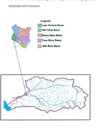
The Nyando catchment is a sub basin of the larger Lake Victoria basin is

located to the east of the shore of lake Victoria in western Kenya. The

catchment is in the south of the Equator at 3S<>.Eand lOS and lies between Lake Victoria to the west, Tinderet hills to the east, Nandi escarpment to

the north and the Mau Escarpment to the south (figure 1.2) shows the

Nyando basin and its sub catchments.

The land slopes generally in the south west direction. The altitude within

the study area varies from about 1000 m above mean sea mean level at

Lake Victoria to over 3000 m above mean sea level in the escarpment

areas.

1

.

2

The Nyando River and its tributaries drain the Nyando River sub-basin

of the Lake Victoria basin. The Nyando River catchment extends over an

area of 33S6km2, ReA (1992). The main channel is River Nyando

starting from the Mau and the Nandi Escarpment forming deep V-shaped

mean sea level. The gradient is steeper upstream than mid and

downstream where it flattens out in the swampy lower areas towards the lake, JICA (1992).

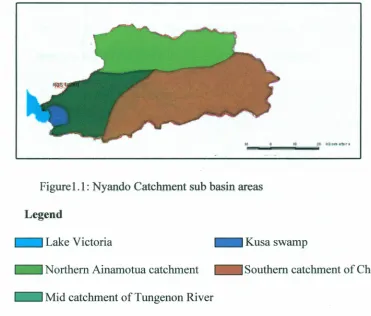
The Nyando catchment may be divided into a number of sub catchments,

but the three distinct ones these are: the northern catchment of the Ainamotua around Tinderet forest which has a drainage area of 840 km2,the mid catchment of river Tungenon which drains an area of 500

km2 and the southern catchment of the Cherongit that drains 900 km2.

The remaining area is part of the Kusa swamp (figure l. 1). There are three main tributaries joining up stream before RGS 1GD03 to form the

main Nyando River channel.

.•

.

..

Figure 1.1 : Nyando Catchment sub basin areas

Legend

Lake Victoria _ Kusa swamp

Northern Ainamotua catchment Southern catchment of Cherongit

1.3 Climate

The climate of Nyando sub-basin area is hot and humid with a mean

annual temperature of 22°C, (Woodhead, 1968). The mean annual

rainfall varies from 1000mm near the lake to over 1600mm in the

highland. The rainfall shows a bimodal pattern, with peaks during March

to May and October to November. These are long and short rainy

seasons respectively.

The rainfall is controlled by the northward movement of the Inter

Tropical Convergence Zone ITCZ. Altitude, proximity to the highlands

and nearness to the Lake shore however cause considerable spatial

variation in the rainfall. The climate of the Lake Victoria region is

therefore hot and wet with the two distinct rainy seasons.

1.4 Geology and Soils

The Nyando catchment area landscape is based on geological structures

such as, rocks, faults, sediments and past geological formations. The

basement consists of the Nyanzian Precambrian system that is overlain

by the Bukoban system, Cole (1950). After several depositions, folding

Bukoban and Nyanzian rocks and subsequent weathering processes, this

has produced different soils with unique physical and chemical

characteristics that cover the region.

The Nyando catchment's physiography is as a result of these geological

processes forming scarps at the rift faults having east-west to east north

east i.e. west to south west direction that shapes the Kavirondo rift that

branch from the main north-south orientation of the Great Rift Valley

systems.

The Nandi and Mau escarpments that are dominated by foot slopes

followed by gently sloping piedmont plains and very flat alluvial plains

dominate the lower catchment of the Nyando. At the base of the scarps,

numerous streams cut deep through the poorly sorted beds of coarse

gravel, sand and sandy clays in the plains. On the upper reaches the

streams gradient are in excess of 20°.

The soils on the plains are derived from Holocene sedimentary deposits,

Andriese and Van Der pouw (1985). These soils are described as

problem soils in terms of management and use, Waruru et al (1992). On the highlands the soils are derived from a variety of parent materials that

The grey and black soils in the Kano plains are mainly found from the

surface alluvial deposits and Pleistocene deposits of sandy red soils

derived from granite found mainly at the foot of the escarpment and on

piedmonts along the escarpment

1.5 Problem Statement

Over the years floods by rivers that drain into Lake Victoria have

occurred, where the most remembered were the historical 1961, WMO (2004). Equally high events have recurred in the 1980's and the 1990's.

Given such frequency of events there is an urgent need to address the

seasonal flooding problem.

A report by nCA (2006) on Nyando basin estimated that the area

perennially affected by flood is about 20,000 hectares and that the floods

do affect about 42,000 persons whenever they occur.

There is need for flood control measures to be implemented. Structural

measures have already been put in place on River Nyando by the

construction of flood control levees, but these have not fully controlled

flooding and its impacts. This is partly because floods are natural and

Though more reassuring; the construction of river bank levees is an

expensive undertaking with an annual recurring cost. The levees

constructed near the banks confine the river flood flow to a defined flood

path. This mode of containment of flood waters denies the biodiversity their needs as they which depend on flood waters of the river when it

spreads out.

The ideal thing would be to develop a management strategy of warning

systems on the river flow to provide alerts of impending flood conditions

on the basin seasonally, based on river basin modeling. This type of approach would provide manageable risk of floods by giving the flood

plain's residents opportunities to use the flood plain and yet stay safe.

Flood warnings and sustainable flood defences will continue to prevent

property damage, loss of life and minimize distress. There is need to

develop an approach to flood management that could improve the

functions of the river basin as a whole; recognizing that floods do have beneficial effects and can never be fully controlled. Such effort should

seek to minimize the negative effects and maximize the flood plain

1.6 Justification

The reason for modeling the Nyando River Basin has been motivated by

the need to provide tools to assist in management solutions to flood

problems within the catchment. At present the river basin lacks adequate telemetry system for operating a real-time forecasting and flood warning

system due to the basin's short lag time, WMO(2004), therefore

necessitating intermediary options.

The conceptual foundation of this multi- disciplinary study approach is

that river flood plains are regional centres of ecological organization.

The system depends on interactions among dynamics, nonlinear physical

and biological processes that relate to water, heat, materials flux and retention to fluvial landscape change.

1

.

7

The main o.!>jective of this research was to determine flood indicator

benchmarks for River Nyando sub-basin from the rainfall-runoff

1.8

SpecificObjectives

a. To determine the rainfall- runoff relationship in Nyando sub basin.

b. To Examine the frequency of flooding in Nyando sub basin.

c. To determine river level threshold that constitute flood threat in the

Sub basin.

d. To identify and zone flood vulnerable areas by modeling.

1

.

9

ResearchQuestions

a What is the relationship between rainfall and stream flow in the Nyando

Sub-basin?

b. At what time intervals does flooding occur in the Nyando sub basin?

c. What are the flood magnitudes and their corresponding river stages?

d. What areas ofNyando sub basin get inundated during flood?

1

.

10

Significanceof the Study

The Nyando River Basin modeling will facilitate zonmg of flood

vulnerable areas. The calibration of the HEC-HMS model on River

and control measures yielding flood maps useful for preparedness

campaigns and awareness.

Legend

Lake Victoria Basin

Rift Valley Basin

::t=

Tana River Basin

" Athi River Basin

Figure 1.2: Nyando sub- basin study area.

CHAPTER

TWO

LITERATURE REVIEW

2 Introduction

Floods refer to water flows or an overflow of streams from their natural or

artificial banks, inundating adjacent low lying areas. Floods are one of the most

common and widespread of all natural disasters. Floods are likely to be a major

concern in the future especially with larger population moving and living near

water courses.

2.1 FloodGenerationProcesses

The rainfall runoff process as described by the kinematic wave method is such that,

the lateral flow is equal to the difference between the rates of rainfall and

infiltration, while the channel flow is taken as flow per unit width of plane, Chow,

V.T.(1988). The characteristic equations that describe the process at the initial are:

aA

aQ

-+-=q

at

ax

(2.1)

(2.2)

aA

at

q I is the discharge, Sf is energy grade line, and So is bed slope

The above equations can be solved to simulate an outflow hydrograph in

response to rainfall of a specified duration. The above kinematic wave

model equation is a one dimensional flow consideration, though when

adjustments are done to the equations they do produce a more realistic

outflow hydrograph (Eie1son, 1970; Overton and Meadows, 1976

Stephenson and Meadows, 1986).

The consequence of a rainfall event usually results in an ever-changing

flow pattern and for that reason a mathematical representation of the

event must include both steady state and non-steady terms.

In rising river water, the advance of the peak: flood wave does not in

general represent the velocity of flowing water. When a flood advances

from the headwaters of a stream, the advancing wave must first fill up

the river channel or immediate valley to the flood line. The peak of the

wave at any point farther down the river is in general caused by water

that has passed any upstream point at a time later than the occurrence of

When a flood is caused by rain, the flood waves may be caused by the local runoff or by combined local and head water runoff; hence the peak of the flood crest in the lower valley may occur earlier or may be simultaneous with the flood crest at points on upper catches. The relative time of the flood crest therefore is entirely a matter of distribution of the rainfall that produces the flood and the flood channel capacity.

From the records of past floods, it is evident that the average flood to be expected every year is exceeded by floods of less frequency, that may occur at intervals of between 5 to 10 years. These will be considerably exceeded by greater floods which may occur at intervals of between 50 to 100 years. Greater floods may follow each other at smaller intervals but the average appearance of the greatest floods is rare and uncertain.

Typically a stream will overflow its normal channel about once in 2 to 3 years and invade low lying places on its flood plains. The overflow occurs when the volume of water entering a stream channel exceeds the hydraulic capacity of the channel.

distribution of rainfall, stream pattern, antecedent moisture condition,

temperature, seasons of the year and the physical features of the

watershed, such as topography, soils geology and drainage pattern,

Waananen et al (1977).

The areas within the Nyando River Basin is characterized by poorly

drained fine textured deep black cotton soils of the clayey soils that are

derived from phonolites. The condition of the soils, the drainage system

and the low lying lands that characterises the plains is a contributor to

water stagnation. Flooding is therefore common occurrence with

frequent periodic inundation of the area after downpours in the

escarpments and the highlands, Orengo et al (2001).

2.2 Floods: The underlying factors

Studies on British rivers and their catchments reported in, Shaw (1994)

showed that catchment characteristics playa major role in flooding and

flood forecasting. The factors evaluated on this study were: size, shape

and area of the catchment; density and distribution of streams; overland

and channel slope; catchments storage, soil and geology, and climate in

The two mam constants in a basin are; land and water and are

interdependent and must be both considered for efficient catchment

management

.

It is also important to note that catchments reflect a

natural unit where there is

interaction of vegetation

,

soil and the

underlying geological formation upon which precipitation provides the

common end products such as runoff, stream flow and ground water,

Singh

(1990).

There are few areas in the world in where runoff has not been affected by

the

influence of man particularly in the tropics.

Apart from vast areas of

rainforest which have been cleared

,

former grasslands have been

ploughed up and swamps have been drained.

There has also been a great increase in urbanization and a resultant

spread of artificial impermeable surfaces. All these activities influence

the response of a catchment area to rainfall and consequently the pattern

and distribution of rainfall and runoff has been altered, Ward and

Robinson (1990).

Human influence on runoff may result from application of specific

agricultural techniques and practices. These practices cause sudden

changes in catchment characteristics for example the vegetative cover in

may be modified substantially by forest cutting and removal procedures,

Ward and Robinson (1990).

The result is that changes within a catchment area have been related to a

modified output of runoff from a catchment, Hewlett & Helvey (1970).

Based on these, one way of understanding the hydrological effects on

land is to relate the effects of land use and manipulation to increase in

severity of floods. The objective of such a study would be to find out

whether flooding is caused by increase in rainfall intensity or duration,

reduced infiltration capacity or a reduced efficiency of the drainage

network.

The disastrous widespread flooding which affected two-thirds of

Bangladesh in September 1980, WMO (2004) are similar to the one

experienced in Nyando basin plains frequently. These may be partially

attributed to large-scale forest removal, deteriorating flood situations or

global climate change. These have caused local alterations in the

frequency of intense or prolonged precipitation and increases in flood

magnitude and frequency.

The available evidence is however largely circumstantial and often

difficult to interpret. It is equally true that land use continuously changes

Flood studies on rivers are essential so as to understand the phenomena

using tools such as runoff models. The models may be deterministic;

where all input, parameters and processes in the model are considered

free of random variation and known with certainty, as in HEC-HMS or

stochastic; where the model describes the random variation and

incorporates the description in the predictions of outputs ,USACE

(2001).

Flood disasters in the Nyando River Basin are a complex construct of the

increasing vulnerability of the population occupying the flood prone

area. The increasing flood instances are caused by heavy rainfall

interacting with hilly slopes on the upper catchments where vegetation

cover is missing yielding flash floods in the vicinity of the foothills.

Other anthropogenic factors such as increased economic use of flood

plains and improved reporting of the impact of floods have given a

perception of increased flood disasters. In the Nyando River Basin, the

factors contributing to increased flood disaster have been identified as

population pressure deteriorating infrastructure and environmental

A study on flooding by The Ministry of Water Resources, Management and Development at the River gauging station 1GD03 on Nyando for the period 1969 to 1997 indicated that flood discharges for different return periods have since increased significantly, MOwn (2004). The study draws inference that during the period 1980 to 1987 the peak discharges had decreased due to the afforestation programs that were undertaken.

In 1997 and 1998, peak discharges increased sharply due to massive destruction of forest cover. The peak discharges could not be attributed to the rainfall patterns, but to catchment characteristics. The understanding of catchment hydrological problems such as floods requires detailed studies using models.

Baseline survey report on Nyando river basin ,JICA (2006) identified various factors that contribute to people's vulnerability to flood manifestation in the Kano plains as: changes in land use in the upper catchment zone, deforestation, channel siltation, catchment deterioration,

reduced vegetative cover and cultivation on steep slopes thus contributing to flush flood at the lower basin.

attributes people's vulnerability to floods to resource scarcity among

other factors.

Flood forecasting and prediction may vary from simple statistical

rainfall- runoff relationship to complex mathematical modeling. The use

and selection of a model depends on data availability, computation

capacity and the basic characteristics of catchment such as time of

concentration. This is the time for runoff to reach its peak, when the

entire water-shed is assumed to be contributing to flow at the outlet

point, Chow (1964).

The application of USGS model for flood forecasting was evaluated on

River Nyando using ground and satellite data, Muthusi (2004).The study identified five river bank sections that were vulnerable to flood breaches

and recommended mapping to determine their extents.

2.3 Models

Models are physical or mathematical representation of a process that can

be used to predict some aspect of the process. Some unknown output is

related to known input. When the Hec-Hms model for example is used in

the rainfall-runoff study, the known input is precipitation and the

flow is the known input while the downstream flow was the unknown

output. Models take a variety of forms such as the linear reservoir

equation, Nash (1957).

S=kQ (2.3)

Where

S is storage and Q is discharge

Physical models are reduced dimensional representation of the real

world system. A physical model of a watershed for example would be a

large surface with overhead sprinkling devices that simulate the

precipitation input, Singh (1998).

2

.

3.1

Categorization of Mathematical Models

Mathematical models may be categorized as event or continuous models.

Other classifications include; lumped or distributed models, conceptual

or empirical, and; deterministic or stochastic models. Event models

simulate runoff from a single storm, the duration of the storm ranging

from a few hours to a few days.

Hec-Hms model uses mostly event models. Continuous models are

models that simulate longer period events such as predicting watershed

In a distributed model the spatial variation of characteristics and

processes are considered explic

i

tly while in a lumped model the spatial

variation are averaged or ignored.

A conceptual model is built upon a baseline of knowledge of the

pertinent physical processes that act on the input to produce the output

.

An

e

mpirica

l

model is built upon observation of input and oU1J?ut

wi

t

h

out seeking to represent explicit the processes, Singh

Models wou

l

d be described as deterministic if all input parameters, and

processes in the model are considered free of random variations and are

known w

i

th certainty. Stochastic models describe random variations and

incorporate the descriptions in their output predictions, USACE

Mathematical models are equations or sets of equations that represent the

response of a hydrological system component to a chang

,

e in hydro

meteorological conditions, USACE

Their presentation in

Hec-Hms program are in part quantitative expressions of a process or

phenomenon being observed, analysed or predicted (Overton and

Meadows,

They represent an idealized situation that has

2.3.2 Hec-Hms model

The Hec-Hms model is a computer program that comprises of a variety

of sub- models that perform various operations of the watershed as; loss

abstractions, runoff transformation, open channel routing, rainfall-runoff

simulation, and parameter estimation.

The program uses a graphical user interface for data input and provides

an integrated analysis platform for the hydrologic components. The

program also provides data storage and management tools with graphic

and reporting facilities.

The choice of the Hec Hms model for the study was based on its scope,

flexibility, ease of data input requirements, ability to accept raw data

without any pre-processing and the wide rage of choices for abstraction

and transformation methods it provides, USACE (2002).

Hec-Hms model was used for catchment hydrological study on river

Kyeekolo in Kaiti Makweni district Kenya to evaluate the application of

hydrological models as tools for water resources planning I?anagement

The study recommended the construction of dams in the catchment to

maximize the use of rain water that runs to waste. It also recommended

afforestation to restore land cover.

2.3.3 Constituents of a Model

Most models including the model Hec-Hms that describes the watershed

response to precipitation have common components:

State variables are tenus in the model equation that represent the state of

the hydrologic system at any particular time and location.

Parameters represent in numerical measure the properties of the real

world that control the relationship of input to system output. They are the

''tuning knobs" of a model as they are adjusted so that the model can

accurately predict the physical system response.

Boundary condition, are values .of a system input. They are the forces that act on the hydrologic system and cause it to change. In Hec-Hms,

precipitation into a watershed is the force which on its application causes

Initial conditions for a model represent the initial state of either soil

moisture in the watershed or the runoff at the start of the storm being

analysed. For a routing model the initial condition is the flow in the

CHAPTER THREE

METHODOLOGY

3 Introduction

This Chapter presents the data collection and analysis methods used in

the study. The methods included; regression and correlation analysis, flood frequency analysis, hydrological modeling and GIS application.

3.1 Data Acquisition and Processing

The data for this research were acquired from various Government

agencies. The hydrological data was obtained from the Ministry of Water

and Irrigation. The rainfall records were obtained from the Kenya

Meteorological Department and the topographic maps were obtained

from the Survey of Kenya.

The daily rainfall and stream flow data acquired from the various sources

were organized on a spreadsheet for each year of record ranging from

1969 to 1997.

The stream flow and rainfall records for the period of the study were

The missing rainfall data were filled up using the weighted average of

four station method, McCuen (1988). The method uses delineation of

four quadrants in the north-south and east-west lines passing th;ough the

rain gauge station in each quadrant which is the nearest to the rain gauge

station with missing data in the quadrant selected. The weights

applicable to each of the four stations are computed as the reciprocal of

the square of the distance between the station and the origin of the

quadrants.

Then the rainfall recorded at the four stations in the four quadrants are

multiplied by their respective weights and added. The resulting sum is

divided by the sum of the weights to yield the missing rainfall.

Px=

1

1

1

1

-

2

P

I

P

2

P3

P4

r,

r2

r3

r4

1

111

-2-+-2 +-2 +-2

r

r

2

r

3

r4

(3.1)

Where Px is the missing station X rainfall.

The mean and standard deviations for each of the variable data set of the

flow discharge and rainfall for the years in record were computed as:

x

1 n

=-Lx;

n ;=1

(3.3)

The rainfall and stream flow stations in the study area are given in Table

3.1and 3.2 respectively whereas all the rainfall data were considered, the

stream flow station with the long term flow records 1GD03 was used

Table3.1 Rainfall stations within Nyando sub-basin

Name 8tationCode Latitudes Longitudes

Kibwani 8935033 00:03'N 36°:06 'E

Ahero 9034086 0°:08' 8 34°:56' E

Songhor 9035009 0°:04' 8 35°:19'8

Kipkeleion 9035020 0°:12' 8 35°:28' E

Tinga 9035188 0°:05' S 35°:27' E

Koru 9035230 0°:08' S 35°:17' E

Table3.2 River gauging Stations within Nyando sub-basin

Station Code Latitudes Longitudes .

IGB03 00°:04':20

-s

"

IGB05 00°:01 ':35" S 35°:10':03" S

IGB06 00°:03':10" S 35°:08':36"

S;

IGBll 00°:01 ':30" S 35°:10':35" E

.

IBC04 00°:15'10" S 35°:24':50 "E

1GC06 00°:12':00" S 35°:28':00" E

IGD03 00°:08':00" S 34°:59':25" E

IGD04 00°:06':05" S 35°:02':40" S

3.2 Data Analysis

3.2.1

Stream flow

From the gauged data for the station, 1GD03 a rating curve was obtained

by fitting a regression between the gauge heights and their corresponding

flows.

The regression took the form: Y=a+bX (3.4)

Where Y is the gauged river flow discharge (m3/s) and X is the gauge

height (m) at the gauging site, a and b are constants

The daily stream flow data were first cumulated to obtain annual flow

volumes. The cumulated annual flow volumes were then transformed to

obtain a regression relationship - between rainfall and runoff. The

transformation of flow volume involves converting the runoff. from flow

rate units to depth by numerical integration of the direct IUIf off quantity at

the gauging site and weighting as;

Depth of direct runoff (mm) =

n

0.36xMIQ;

1=;

A

Where A is the catchment area ( m2)

3.2.2 Rainfall

The daily point rainfall data were converted to mean areal rainfall using

the Thiessen (1911) polygon weighting method. The Thiessen polygon

weights are obtained by connecting adjacent stations on a catchment map

by straight lines and erecting perpendicular bisectors to each connecting

line. The polygon formed by the perpendicular bisectors around a station

encloses an area which is anywhere closer to the station than any other

station. The area is taken to be best represented by the precipitation at the

enclosed station.

Based on this approach, the Thiessen method transforms individual

station point rainfall to catchment areal rainfall. The areal rainfall

computed on daily basis is then cumulated to obtain mean areal rainfall

for the basin.

- ~pa

The mean areal rainfall is computed as: p =~ -' -'

;=J A

(3.6)

Where:

Pi is the station precipitation

a, is the enclosed polygon area around station i

The Thiessen method transforms individual station point rainfall to

catchment areal rainfall. The computed areal daily rainfall is then

cumulated to obtain mean annual areal rainfall for the basin.

3.2.3

The correlation coefficient of the data set was estimated as:

i n

rij=

~:CXi

~:CYj _

i=! j=!

(3.7)

x

is meanofx

Y

is mean ofy

Sx

is the standard deviation of x

S, is the standard deviation of y

A regression relationship between the two variables X and Y was

obtained by an equation of the form given in equation 3

.

4 where X is the

dependent variable.

The regression objective was two fold. First it served to determine the

rating curve equation for the RGS data of gauge height and measured

discharge (3.2.1), and secondly it was to establish rainfall-runoff

3.3 Frequency Analysis

Flood Frequency analysis is one the most important studies of river

hydrology. It seeks to use past records to determine the probability of

occurrence of extreme events. The magnitude of extreme floods can be

related to their frequency of occurrence through the use of a probability

distribution.

The selection of a distribution function to describe a random variable is

based on observed historical data and the underlying physical

phenomenon. For describing the peak discharges series, the extreme

.

value type 1 distribution is the most suitable.

The uncertainties associated with hydrological events are overcome by

evaluating and assessing the probability that the output variable of

interest will exceed some set target level by using a probability density

function (pdf) and cumulative distribution function (cdf) to describe the

event.

The data analysis for extreme peak discharge series relies on the

selection of the distribution type. The type of distribution that is suitable

1996). The general extreme value (GEV) distribution types such as the

extreme value type 1,use the cumulative density function (cdf)'to defme

the event probability.

In this study the type 1 distribution was used to plot the peak discharges

against their probabilities of non-exceedence. The cumulative probability

distribution (cdf) is described as:

[ x-u]

F(X)=exp -1(~) (3.8)

The same expressed as a probability density function (pdf) is:

1

[x-u

x-u]

f (x) = -exp - -- - exp(--)

a

a

a

The mean f.i and the variance a in the Gumbel distribution equation are

related to the location parameter

u

a,

and Huber, 1988)

u= u

+

0.5777a

and

(3.11)

The parameters transformation makes it possible to express the

standardized variate

x-u

Y

T=

--a

The Variant was then transformed as a form of cumulative distribution

function express as:

G(Yr)

=

The transformed variables make the plot of the variables on an ordinary

scale possible.

The distribution graph is then plotted with the extreme discharges on the

ordinate and the variant or the return period on the.abscissa. The values

of the variant for plotting are computed based on the return period as

YT=-ln[ -In(1- ~)]. (3.14)

The extreme value type 1 introduced by Gumbel (1941) is one of the

widely used probability analysis for extreme values in hydrological

events. The distribution is based on building a relationship between the

probabilities of the occurrence of an event, its return period and the

magnitude of the extreme hydrological events such as floods.

The distribution is based on a theoretical interpretation for describing

the physical process of the hydrological phenomena where hydrological

analyses are asymptotic and are valid only for large and independent

The peak stream flow as described by Gwnbel distribution considers the

daily flow as a statistical variable unlimited to positive end of the

distribution having defined a flood as the largest value of the 365 daily

flows. Based on the theory of e

x

treme flows the annual largest values of

a nwnber of years of records approaches a definite pattern of frequency

dist

r

ibution and can be

f

itted

i

n a theoretical extremal distribution of

type

l.

Th

e

extreme value distribution is justified only when it is shown that the

val

u

e

of the daily discharges follows an exponential type distribution.

The annual peaks selected were the largest of the 365 daily discharges

and the numbers in record is large enough for the asymptotic theory to

apply. The probability of an event Q being less than X is expressed as:

f ( ) [X - u ] e-y

Q<x

exp - e

x

p(

-

~)

-

=

e-

(3

.

15)

Y

T

reduced variate

(3.16)

3.3.1 Fitting a Distribution

There are three models that are commonly used for extreme value

analysis. These are Gwnbel

,

Frescher and Weibull distribution functions.

scale parameters while others need shape parameter as well

.

order to

determine whether or not a particular sample from a population fits a

Gumbel or other probability distribution a plot that produces points that

fall close to a straight line assures that the fitted distribution is the

reasonable model

,

Devore (2002)

.

To

ex

amine the frequency of flooding of Nyando River, a Gumbel

pro

ba

bility plot of extreme peak discharges for RGS 1GD03 was done.

Th

e f

itting of the

extreme peak flow records on a Gumbel distribution

cu

r

v

e

was achieved by using the Weibull plotting method.

The Weibull method assigns probability and return periods for the data

set by sorting them in series in ascending order of magnit;Ide. The basis

of this is that the probability

p

is related to the return period T of the

flood and that the plotting position or variate is related to the flood

magnitude

.

3.3.2 Plotting position

The peak discharge series set was ranked for the analysis by the Weibull

method to compute the probability and the corresponding return periods.

in descending order. The probability of each observation is computed as

m

pl=

-n+1 (3.17)

Where pl is the left sided probability (probability of having les~ than the

series)

m

=

N= number of observation.

The return period for each observation is computed as

T=N

+

m

Where T =the return period

N=total number of items in the set

m

=

The plotting position of the observation of the extreme peak discharge is

in the ordinate and the variant YT expressed as

1

Y =-ln[-In(--)]

T ~()()

(3.19)

Other than defining the reduced variate in terms of probability the same

can be based on the return period selected T where the reduced variate

YT is computed in terms ofthe return period for the left hand probability

as:

(3.20)

The variate for right-hand probability can also be computed in

YT=

-Ln

[In(~)J

T-1 (3.21)

The application of recorded data "beyond the existing records requires

data extension by extrapolation with reliable means. This was done for

values that were out side the range of the recorded data -based on the

extreme value distribution of the type 1 using the',frequency factor

method.

The extreme value type 1 distribution, Gumbel's gives the probability of

-•.-Y

being exceeded as

P

The type 1 distribution, a part from fitting of the Gumbel line also

describes a T- year flood with an equation as:

-XT= X +

(0.7797Y

T

- 0

.

45005) Sx

Any flood of magnitude X for any return period T may be computed as:

(3.24)

Where

KT

Kr = _

J6(r+Lnln

r(x) )

7r

T(k -1)

The floods usually fallon the mean line, therefore a standard error of

estimate is used to compute for the values that fall on the envelope lines

on both sides of the mean line. The computation for the error ~as based

on a 95% confidence limit for the't' test distribution as:

1

S

-SE (XT)=

2

..

[1

+

+

1

r

N (3.26)

3.4

HydrologicModeling

The Hydrologic modeling was done using HEC-HMS model

(version2.2.2), a computer program, which defines a river basin by state

variables, initial conditions, boundary conditions and parameters. The

Hec-Hms model was found suitable for the study of a large river basin

covering an area of 2665 km2 starting from the control point at RGS

1GD03 upstream.

The area under study was defined by the drainage pattern, hydro climatic

data, and operational controls. The program provided working platforms

that made it possible to create the various components of the basin

namely: hydrologic elements in the basin model, meteorologic model

The Hec-Hms model version used for this study provided analytical

tools that converted point rainfall to mean areal rainfall, mean areal

rainfall to a temporal distributed mean areal rainfall, a temporal

distributed mean areal rainfall to a hyetograph and hyetograph to

hydrograph.

3.4.1

Hec-HMS Modeling Components

The Hec-Hms model is a hydrologic model developed by the Hydrologic

Engineering Centre. The program simulates the surface runoff response

of a river basin to precipitation by representing the basin as an

interconnected system of hydrologic and hydraulic components such as

sub basin, streams channels, sinks and reservoirs. The Hec-Hms uses

separate model to represent each component of the runoff process such

as runoff volume, direct runoff arid channel flow.

3.4

.

1.1

Runoff Volume

In the Hec-Hms , runoff volumes may be computed using any of the

following; Initial and constant- rate, SCS curve number (CN), Gridded

SCS CN, Green and Ampt, Deficit and constant rate or Soil Moisture

event, lumped, empirical distributed, empirical, or fitted parameter

models.

The runoff volume model addresses the questions about the volume of

precipitation that falls on the watershed by interrogating, how much

infil

t

ration is on pervious surface, and how much runoff comes from the

impe

r

vious surface, and how it runs off

.

Th

e

program provides many choices of carrying out that computation.

Th

e

Nyando study the Green & Ampt was used. The Green &

'

Ampt is a

conceptual model of infiltration of precipitation in a watershed. The

model computes the precipitation loss on the pervious area in a time

interval as:

(3.27)

Where

f

is loss during period t

,

( mm)

k is saturated hydraulic conductivity,

( ¢ - B )

Volume moisture deficit

Sf

is wetting front suction, (mm)

The parameters that were estimated to model with the Green &Ampt

equation are; initial loss, hydraulic conductivity, wet front suction and

volume moisture deficit.

The initial loss is the parameter designating a function of the watershed

moisture at the begirming of the precipitation US ACE, (2002). It may be

estimated in the same manner as the initial abstraction. The hydraulic

conductivity is the parameter derived as a function of texture class.

The wetting front Suction is the parameter that is estimated as a function

of pore size distribution and also texture class. The volume moisture

deficit (¢ - B) is the parameter that defines the soil porosity less the

initial content according to Rawls and according to Brakensiek, (1982)

3.4.1.2 Loss' Rate

The basin loss rate applied in the program is based on the fact,that all the

land and water in a watershed can be categorized as either directly

connected impervious surface or pervious surface. The impervious

surface was that part of the watershed for which all the precipitation

runoff with no infiltration, interception, evaporation, or other losses the

precipitation to the pervious surface was subject to losses.

In

specified as percent imperviousness. The selection was on the basis that

the loss method was more physically based in approach to infiltration of

water into the soil.

The Green and Ampt.method was considered ideal for Nyando Basin

study as the parameterization method are derived as functions of soil

class texture, soil porosity and initial water content which were possible

to relate to a largely rural basin. The Green and Ampt method modelled

infiltration by the combining an unsaturated flow from Darcy's law with

the requirement of mass conservation.

The parameters for the Green and Ampt that were specified in the model

are; initial loss in mm, volume moisture deficit ratio, wet front suction in

mm, and conductivity in mmIh and percent imperviousness. The concept

was that once the initial loss has accounted for interception and

depression storage, the excess precipitation is computed using the Green

and Ampt equation.

3

.

4

.

2 Direct Runoff

The Hec-Hms uses various direct runoff models such as the user

specified unit hydro graph (UH), Clark's, Snyder's, SCS UH, ModClark,

lumped, empirical, fitted parameter, measured parameter models. In this

study the Snyder's UH is used.

The model Hec-Hms simulates direct runoff of excess precipitation on a

watershed using transforms, which "transforms the excess precipitation

into point runoff'. The option for the process in the program uses

conceptual models such as the unit hydro graph, the kinematic

-wave

model. The direct runoff was computed based on the unit hydro graph transform.

The unit hydro graph method on its part is an empirical relationship of

direct runoff to excess precipitation that was originally proposed by

Sherman in 1932, as the basin outflow resulting from one unit of direct

runoff generated uniformly over the drainage area at a uniform rainfall

rate during a specific period of rainfall duration (USACE, 2000).

The computation as done by the model Hec-Hms is on the discrete

representation of excess precipitation in which "pulse" of precipitation is

known for each time interval and based on that it then solves the discrete

convolution equation for linear system as:

nsM

Q

LPmUn-m

m=l

(3.28)

Where

Pm

=

m= total number of discrete rainfall pulses; and

Un-rn+1 = UH ordinates at time (n-m+ 1) ~ t.

Qnand Pmare flow and depth respectively.

The use of the equation was in the implicit assumptions that were made

in the model.

The unit hydro graph equation applied for the transform was the

parametric unit hydrograph developed by Snyder in 1938 (USACE2000).

The Snyder Unit Hydrograph (figure 3.1), was an event lumped,

empirical, fitted parameter model that had characteristics that are related

to the watershed characteristics. The form of Snyder unit hydro graph

method as used in the Hec- Hms model uses the Clarke unit hydrograph

method to compute the hydro graph ordinates.

The Clarke method on its part uses the Snyder unit hydro graph to select

the lag time; peak flow and total time base flow as the critical

characteristics of the Unit graph. The parameters that were estimated for

the Snyder Unit Hydrograph were UH lag tp and coefficient CpoThe time

to peak, tp may be expressed as;

tp=CCt (LLc)O.3 _(3.29)

Where

L=length of the main stream from the outlet to the divide;

L, =length a long the main stream from the outlet to a point nearest the

watershed centroid;

C= a conversion constant

Cp is calibrated at from 0.1 to 1

The transform method is used

tq

rainfall that is based on the fact that precipitation that did not infiltrate or

felt on directly connected imperviousness surface becomes excess

precipitation.

While excess precipitation can remain on the surface in depression or

ponds, it typically moves down-gradient on the watershed land surface

and becomes direct runoff. In the transform method, the Snyder unit

hydro graph was used to compute direct run off from the excess

precipitation.

The parameters for the Snyder transform are the Snyder standard lag,

Snyder peaking coefficient cp both in units of time as indicated in figure

:_t

p

-.

Discharge per urut excess precipitation

depth

Time

Figure 3.1: Snyder's unit hydrograph

(Source: USACE Technical reference manual, 2000)

3.4.2.1 Base flow

The Hec-Hms provides a number of methods to compute base flow these

include the Constant monthly varying value, Exponential recession and

linear reservoir volume accounting. The base flow models are described

as; event, lumped, empirical or fitted parameter models. In this study the

exponential recession method was used to determine the base flow

recession.

The parameterization for the sub basin to account for the base flow was

based on the fact that water that infiltrate through the soil in a watershed

passes through the unsaturated vadoze zone and enters the ground water.

Ground water is rarely static but slowly moves down gradient through

The movement of ground water makes them

the principle source of

stream flow during dry periods as it returns to the stream channel directly

from beneath. The ground water flow that returns to the stream is the

base flow. That quantity of returned ground flow was modelled by

recession method

.

The

method was considered suitable for the base flow

modeling as it uses an exponentially declining base flow that applies

clas

s

ic separation techniques.

The parameters for the recession base flow are the initial flow that was

defined by a point on the hydrograph when it appeared that the runoff

took over as the main flow on the rising limb, a recession constant that

defines decay rate, and the threshold flow that defines the point on the

hydrograph where base flow becomes the major flow on the falling limb

of the flood hydrograph.

3.4.3 Channel flow

The Hec-Hms provides a number of methods to compute channel flow.

These

are;

Kinematic

wave,

.

Lag,

Modified

plus,

Muskingum,

confluence and bifurcation

.

These channel flow models are described as

;

event

,

lumped

,

conceptual

,

measured parameter, quasi- conceptual and

continuous model

.

In this study the Muskingum-Cunge standard section

was used

.

Routing with Hec-Hms was carried out when the various stream reach on

the b

asi

n model were parameterized so that they could represent the flow

of w

at

e

r in the open channel

.

The routing process relies on the concept

that

w

ater requires a certain amount of time to travel down a reach.

In the channel a flood wave is attenuated by friction and channel storage

as it passes through a reach. The process of computing the travel time

and attenuation of water flowing in the reach is routing. The parameters

that were specified for a reach to compute travel time and attenuation

using Muskingum-Cunge Method are; reach length in (m), water energy

slope (m/m), stream bottom width (m), side slope and Manning's number

.n. Hec-Hms model provides other options for channel routing other

than the Muskingum- Cunge standard method used here.

This form of routing computes downstream hydrograph for a given

upstream boundary condition based on the solution of the continuity

aA aQ

equa

t

ion -

+ -

=

and the diffusion form of the momentum

at

Ox

Sf

=

ax

the convective diffusion equation

aQ

aQ

a

Q

-+c-=j.1-+cq (3.30)

at

ax

ax

j.1

= ~

=

=

aQ

=

=

zs«

,

aA

water surface

A finite difference approximation of the partial derivative combined with

these coefficients gives discharge as

Q

)1+[

]1

2k(1- x)

+

xr+

+

The solution of the constants yields the Muskingum - Cunge routing

equation in tlie form for the fust reach:

(3.32)

The Muskingum - Cunge Routing equation may be solved by other

approaches other than the equations above in the form of a linear scheme

by solving a time space computational grid figure 3.2, where the

time t where x

=

=

Q

L~l=

C1Q

t

Q

j

C

Q

!

(3

.

33)

Timet

jAt

Qj+l

1+1

i+l

QJ, Ax

I !

'---'---'---+ Distance x

i& (i+1)&

Figure 3.2: Finite difference method space-time grid solution for

Muskingum- Cunge flow computation (chow, (1988)

o

o

The reach outflow as computed with equation 3.31 and equatio~ 3.32 are

modified to

O,

C/

C

1

C

0

(3

.

34)

with the coefficients to the equation given as:

M-2KX

C

=

2KX(1-X)+M

C _ i1!+2KX

2 - 2K(1-X)+M

(3.35)