Early fetal weight estimation with expectation maximization algorithm

(1)

Early fetal weight estimation with expectation maximization

algorithm

Loc Nguyen

Sunflower Soft Company, An Giang, Vietnam Email: [email protected]

Thu-Hang T. Ho

Vinh Long General Hospital, Vinh Long, Vietnam Email: [email protected]

Abstract

Fetal weight estimation before delivery is important in obstetrics, which assists doctors diagnose abnormal or diseased cases. Linear regression based on ultrasound measures such as bi-parietal diameter (bpd), head circumference (hc), abdominal circumference (ac), and fetal length (fl) is common statistical method for weight estimation but the regression model requires that time points of collecting such measures must not be too far from last ultrasound scans. Therefore this research proposes a method of early weight estimation based on expectation maximization (EM) algorithm so that ultrasound measures can be taken at any time points in gestational period. In other words, gestational sample can lack some or many fetus weights, which gives facilities to practitioners because practitioners need not concern fetus weights when taking ultrasound examinations. The proposed method is called dual regression expectation maximization (DREM) algorithm. Experimental results indicate that accuracy of DREM decreases insignificantly when completion of ultrasound sample decreases significantly. So it is proved that DREM withstands missing values in incomplete sample or sparse sample.

Keywords: fetal weight estimation, regression model, ultrasound measures, expectation maximization algorithm.

1. Introduction

According to the regression approach of fetal weight estimation, without loss of generality, an estimation formula is a linear regression function Z = α0 + α1X1 + α2X2 + … + αnXn where Z is

estimated fetal weight whereas Xi (s) are gestational ultrasound measures such as bi-parietal

diameter (bpd), head circumference (hc), abdominal circumference (ac), fetal length (fl). Variable Z is called response variable or dependent variable. Each Xi is called regression

variable, regressor, predictor, regression variable, or independent variable. Each αi is called

regression coefficient. Researches focusing on the regression approach aim to estimate coefficients from gestational sample of ultrasound measures. For example, Hadlock et al. (Hadlock, Harrist, Sharman, Deter, & Park, 1985) proposed regression models for weight estimation based on head size, abdominal size, and femur length, which is better than those based on measurements of head and body. Error means in percentage of their models are 1.3%, 1.5%, 0.4%, 1.4%, 2.3%, and –0.7% whereas error standard deviations are 10.1%, 9.8%, 7.7%, 7.3%, 7.4%, 7.3%.

Phan (Phan, 1985) proposed some amazing regression formulas for estimating fetal age and weight based on bpd, hc, ac, abdominal area (aa), abdominal diameter (ad), average abdominal diameter (aad). Pham (Phạm, 2000) proposed some amazing regression formulas for estimating fetal weight based on bpd, ad, arm length (al), abdominal diameter (ad), average abdominal diameter (aad). Ho (Ho T. T., Nghiên Cứu Phương Pháp Ước Lượng Trọng Lượng Thai, Tuổi Thai Bằng Siêu Âm Hai và Ba Chiều, 2011) produced some amazing regression formulas for

(2)

estimating fetal age and weight based on bpd, ac, hc, thigh volume, and thigh volume in her PhD dissertation. Some of Ho’s formulas (Ho T. T., Nghiên Cứu Phương Pháp Ước Lượng Trọng Lượng Thai, Tuổi Thai Bằng Siêu Âm Hai và Ba Chiều, 2011) are log(weight) = 1.746 + 0,0124*bpd + 0,001906*ac with R = 0.962, weight = –13099.1862 + 125.662*ac – 0.3818*ac*ac + 0.00045*ac*ac*ac with R = 0.9247, weight = –3306 + 55.477*bpd + 13.483*thigh_volume with R = 0.9663, age = 167.0791 – 1,5537*ac + 0.00556*ac*ac – 0.00000618*ac*ac*ac with R = 0.8980, age = 331.0223 – 1.6118 * (hc + ac) + 0.0028 * (hc + ac) * (hc + ac) – 0.0000015 * (hc + ac) * (hc + ac) * (hc + ac) with R = 0.9212, age = 21.1148 + 0.2381 * thigh_volume – 0.001 * thigh_volume * thigh_volume + 0.000002 * thigh_volume * thigh_volume with R= 0,9959. Note that log(.) denotes logarithm function and R is correlation coefficient. The larger the R is, the better the formula is.

Deter, Rossavik, and Harrist (Deter, Rossavik, & Harrist, 1988) reassessed the weight estimation procedure of Rossavik (regression analysis) with particular emphasis on parameter estimation and performance over a wide weight range. As results, Deter, Rossavik, and Harrist assured that “there is no systematic errors over a 250 gram to 4750 gram weight range and random errors (± l standard deviation) of 10% to 13% below 200 gram and 6% to 8% above 2000 gram. The weights of small-and large-for-gestational age fetuses were systematically overestimated (4.1%) and underestimated (–3.0%), respectively, but systematic errors were not found in average-for-gestational age fetuses”.

Varol et al. (Varol, Saltik, Kaplan, Kilic, & Yardim, 2001) evaluated the growth curve of well-functioned regression models (Hadlock formulas, for example). Their purpose is to contribute to develop national standard growth curve of gestational age and birth weight. Percentile values and correlation coefficients were calculated and well-functioned regression models were produced for growth curve. As a result, the regression model for gestational age age = 4.945 + 0.606*ac + 0.105*bpd + 0.286*fl with adjusted R2 = 0.937 is optimal.

Salomon, Bernard, and Ville (Salomon, Bernard, & Ville, 2007) used polynomial regression approach to compute a new reference chart for weight estimation. Their resulted birth-weight chart showed that the weight estimation was noticeably larger at 25 – 36 weeks. At 28 – 32 weeks, the 50th centile of actual birth weight is approximated to the 50th centile of estimated weight.

A. R. Akinola, I. O. Akinola, and O. O. Oyekan (Akinola, Akinola, & Oyekan, 2009) evaluated many regression estimation models. Their results showed that models with hc and ac are not as good as those with ac and bpd. The combination of fl and ac did not improve accuracy. The uses of multiple measures gives most accurate estimation.

Lee et al. (Lee, et al., 2009) used multiple linear regression model with standard measures (bpd, fl, ac) and their proposed biometrics such as fractional arm volume (fav) and fractional thigh volume (ftv). They produced six weight estimation models such as model 1, model 2, model 3, model 4, model 5, and model 6. The model 3 which is log(weight) = 0.5046 + 1.9665*log(bpd) – 0.3040*log(bpd)*log(bpd) + 0.9675*log(ac) + 0.3557*log(fav) and model 6 which is log(weight) = –0.8297 + 4.0344*log(bpd) – 0.7820*log(bpd)*log(bpd) + 0.7853*log(ac) + 0.0528*log(ftv)*log(ftv) gain highest accuracy. Model 5 classified an additional 9.1% and 8.3% of fetuses within 5% and 10% of birth weight. Model 6 classified an additional 7.3% and 4.1% of infants within 5% and 10% of birth weight.

(3)

Note that their two-dimension model is weight = –562.824 + 11.962*ac*fl + 0.009*bpd*bpd*ac*ac. Their three-dimension models are weight = 1033.286 + 12.733*thigh_volume and weight = 1025.383 + 12.775* thigh_volume.

Cohen et al. (Cohen, et al., 2010) used linear regression model to compare estimated weights for births after 6 days after last ultrasound scan and actual weights. Their results indicate that the mean ± standard deviation percentage among deliveries within 1 day of last ultrasound scan is 0.2 ± 9%.

Siggelkow et al. (Siggelkow, et al., 2010) proposed a new algorithm of isotonic regression to construct a birth weight prediction function that increases monotonically with each of input variables (ultrasound measures) and minimizes empirical quadratic loss. As a result, their isotonic regression function gains a small mean absolute error (312 gram).

Pinette et al. (Pinette, et al., 1999) used mean weight value from multiple formulas in order to improve the estimation. For instance, Pinette et al. calculated four estimated weight values w1, w2, w3, and w4 from formulas of Shepard, Hadlock, and Combs and then, they computed

the mean w = (w1 + w2 + w3 + w4) / 4 as the optimal estimated value of birth weight.

When fetal weight is estimated based on gestational age, the weight-for-gestational chart is used. In such chart, if gestational age falls below 10th percentile then, it is impossible to estimate respective weight and so such problem is called small-for-gestational-age which often occurs because of missing data. Hutcheon and Platt (Hutcheon & Platt, 2008) applied standard epidemiologic approaches to correct the missing data problem. However such approaches does not use regression model. When gestational age is incompletely recorded, Eberg, Platt, and Filion (Eberg, Platt, & Filion, 2017) proposed four approaches to estimating missing gestational age: (1) generalized estimating equations for longitudinal data; (2) multiple imputation; (3) estimation based on fetal birth weight and sex; and (4) conventional approaches that assigned a fixed value (39 weeks for all or 39 weeks for full term and 35 weeks for preterm).

In general, most of researches required that the time point to take ultrasound measures is not too far from last ultrasound scan so that bias of actual birth weight at delivery time is small enough. If ultrasound examinations are taken soon, the gestational sample will lack weights because ultrasound measures do not conform to actual birth weight at delivery time. In the next section, we propose an algorithm which is an application of expectation maximization (EM) algorithm for estimating fetal weight in case of incomplete data. Here we should survey some researches related to how to apply EM algorithm into regression model. In literature of EM algorithm, missing values of data sample are estimated in expectation step and coefficients of regression model are re-estimated in maximization step. For example, Zhang, Deng, and Su (Zhang, Deng, & Su, 2016) used EM algorithm to build up linear regression model for studying glycosylated hemoglobin from partial missing data. In other words, they aim to discover relationship between independent variables (predictors) and diabetes. Therefore, the ideology of applying EM algorithm into regression model is not new but we propose a special technique to construct mutually two dual regression models at the same time from incomplete gestational sample. The algorithm that implements such technique is called dual regression expectation maximization (DREM) algorithm. DREM simplifies EM algorithm with assumption of normal distribution and moreover only weights in gestational sample are missing. DREM is described in next section.

2. Methodology

(4)

performed after 28-week old fetal age. In the chapter “Phoebe Framework and Experimental Results for Estimating Fetal Age and Weight” of the book “E-Health” by Thomas F. Heston, we proposed an early weight estimation in which ultrasound measures can be taken before 28-week old fetal age. In this research, we implement such proposal as a so-called dual regression expectation maximization (DREM) algorithm and then make experiments on DREM. With DREM, the gestational sample can be totally collected at any appropriate time points in gestational period. In other words, the sample can lack fetal weights. This is a convenience for practitioners because they do not need to concern fetal weights when taking ultrasound examinations. Consequently, early weight estimation is achieved. As a convention, vectors are column vectors if there is no additional information.

Suppose we estimate two linear regression models Z = α0 + α1X1 + α2X2 + … + αnXn and Z

= β0 + β1Y where Z is fetal weight and Y is fetal age whereas Xi (s) are gestational ultrasound

measures such as bpd, hc, ac, and fl. Suppose both random variables Y and Z conform normal distribution, according to equation 1 (Lindsten, Schön, Svensson, & Wahlström, 2017, pp. 8-9). Note, only Z is random variable whereas X and Y are data.

𝑃(𝑍|𝑋, 𝛼) = 1

√2𝜋𝜎₁2exp (−

(𝑍 − 𝛼𝑇_𝑋)2

2𝜎₁2 )

𝑃(𝑍|𝑌, 𝛽) = 1

√2𝜋𝜎₂2exp (−

(𝑍 − 𝛽𝑇_{(1, 𝑌)}𝑇₎2

2𝜎₂2 )

(1)

Where, α = (α0, α1,…, αn)T and β = (β0, β1)T are parameter vectors where X = (1, X1, X2,…, Xn)T

and (1, Y)T are data vectors. As a convention, linear function Z = α0 + α1X1 + α2X2 + … + αnXn

is called first function, first model, or first formula whereas linear function Z = β0 + β1Y is

called second function, second model, or second formula. Such two models are estimated in duality at the same time. The means of Z with regard to the first model and the second model are αT_{X and β}T_{(1, Y)}T_{, respectively whereas the variances of Z with regard to the first model}

and the second model are σ12 and σ22, respectively. Note that the superscript “T” denotes

transposition operator in vector and matrix.

Let D = (X, y, z) be collected sample in which X is a set of sample measures, y is a set of sample fetal ages, and z is a set of fetal weights with note that z is empty or incomplete. If z is empty, there is no zi in z. If z is incomplete, z has some values but there are also some missing

values in z. However, the constraint is that X is complete. Now we focus on estimating α and β based on D. As a convention let α*_{and β}*_{be estimates of α and β, respectively (Lindsten,}

Schön, Svensson, & Wahlström, 2017, p. 8).

𝑿 = ( 𝒙₁𝑇

𝒙₂𝑇

⋮ 𝒙_𝑁𝑇

) = (

1 𝑥₁₁ 𝑥₁₂ ⋯ 𝑥_1𝑛 1 𝑥21 𝑥22 ⋯ 𝑥2𝑛

⋮ ⋮ ⋮ ⋱ ⋮

1 𝑥𝑁1 𝑥𝑁2 ⋯ 𝑥𝑁𝑛

)

𝒙_𝑖 =

( 1 𝑥₁₁ 𝑥12

⋮ 𝑥1𝑛)

, 𝒚 = ( 𝑦₁ 𝑦₂ ⋮ 𝑦_𝑁

) , 𝒛 = ( 𝑧₁ 𝑧₂ ⋮ 𝑧_𝑁

)

Given X and Y, the entire probability of Z is defined product of P(Z | X, α) and P(Z | Y, β) according to equation 2.

𝑃(𝑍|𝑋, 𝑌, 𝛼, 𝛽) = 𝑃(𝑍|𝑋, 𝛼)𝑃(𝑍|𝑌, 𝛽)

= 1

2𝜋√𝜎₁2_𝜎 22

exp (−(𝑍 − 𝛼

𝑇_𝑋)2

2𝜎₁2 −

(𝑍 − 𝛽𝑇_{(1, 𝑌)}𝑇₎2

(5)

Conditional expectation of sufficient statistic Z given X with regard to P(Z | X, α) is specified by equation 3.

𝐸(𝑍|𝑋) = 𝛼𝑇_𝑋 ₍₃₎

Conditional expectation of sufficient statistic Z given Y with regard to P(Z | Y, β) is specified by equation 4.

𝐸(𝑍|𝑌) = 𝛽𝑇_{(1, 𝑌)}𝑇 ₍₄₎

Equation 2 indicates both explicit dependence via P(Z | X, α) and implicit dependence via P(Z | Y, β). There is a heuristic assumption that the explicit dependence and the implicit dependence share equal influence on Z if E(Z | X) specified by equation 3 is equal to E(Z | Y) specified by equation 4. Let E(Z | X, Y) be the expectation of Z with regard to the entire probability of Z specified by equation 2. If the heuristic assumption is satisfied, we have E(Z | X, Y) = E(Z | X) = E(Z | Y). This implies 2E(Z | X, Y) = E(Z | X) + E(Z | Y). Thus, from equations 3 and 4, we have equation 5 to specify the heuristic assumption.

𝐸(𝑍|𝑋, 𝑌) =𝛼𝑇𝑋 + 𝛽𝑇(1, 𝑌)𝑇

2 (5)

Please pay attention to equation 5 because Z will be estimated by such expectation later. For convenience, let Θ = (α, β)T_{be the compound parameter. The entire probability of Z}

given X and Y specified by equation 2 is re-written as follows:

𝑃(𝒛|𝑿, 𝒚, Θ) = 𝑃(𝒛|𝑿, 𝛼)𝑃(𝒛|𝒚, 𝛽)

= ∏ 𝑃(𝑧𝑖|𝒙𝒊, 𝛼)𝑃(𝑧𝑖|𝑦𝑖, 𝛽) 𝑁

𝑖=1

(Due to all observations are independently and identically distributed)

= ( 1 2𝜋√𝜎₁2_𝜎

22

)

𝑁

∗ exp (−1 2(∑

(𝑧𝑖 − 𝛼𝑇𝒙𝑖)2

𝜎₁2 𝑁

𝑖=1

+ ∑(𝑧𝑖− 𝛽

𝑇_{(1, 𝑦} 𝑖)𝑇)2

𝜎₂2 𝑁

𝑖=1

))

The log-likelihood function is logarithm of the entire joint probability according to equation 6.

𝐿(Θ) = log(𝑃(𝒛|𝑿, 𝒚, Θ))

= −𝑁log(2𝜋) −𝑁log(𝜎12)

2 −

𝑁log(𝜎₂2₎

2 −

1

2𝜎₁2∑(𝑧𝑖− 𝛼𝑇𝒙𝑖)2 𝑁

𝑖=1

− 1

2𝜎₂2∑(𝑧𝑖− 𝛽𝑇(1, 𝑦𝑖)𝑇)2 𝑁

𝑖=1

(6)

The optimal estimate Θ* is a maximizer of L(Θ), according to equation 7 (Lindsten, Schön, Svensson, & Wahlström, 2017, p. 9).

Θ∗ _{= argmax}

Θ 𝐿(Θ) (7)

By taking first-order partial derivatives of L(Θ) with regard to Θ (Nguyen, Matrix Analysis and Calculus, 2015, p. 34), we obtain:

𝜕𝐿(Θ) 𝜕𝛼 =

1

𝜎₁2∑(𝑧𝑖 − 𝛼𝑇𝒙𝑖)(𝒙𝑖)𝑇 𝑁

𝑖=1

𝜕𝐿(Θ) 𝜕𝛽 =

1

𝜎₂2∑(𝑧𝑖 − 𝛽𝑇(1, 𝑦𝑖)𝑇)(1, 𝑦𝑖) 𝑁

𝑖=1

(6)

{

∑(𝑧𝑖 − 𝛼𝑇𝒙𝑖)(𝒙𝑖)𝑇 𝑁

𝑖=1

= 𝟎𝑇

∑(𝑧𝑖 − 𝛽𝑇(1, 𝑦𝑖)𝑇)(1, 𝑦𝑖) 𝑁

𝑖=1

= (0,0)

(8)

The notation 0 = (0, 0,…, 0)T denotes zero vector. All equations in the system 8 are linear, whose unknowns are Θ = (α, β)T_.

We apply expectation maximization (EM) algorithm into estimating Θ = (α, β)T_{with lack}

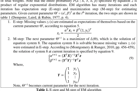
of fetal weights. Note that the entire probability P(Z | X, Y, α, β) specified by equation 2 is product of regular exponential distributions. EM algorithm has many iterations and each iteration has expectation step (E-step) and maximization step (M-step) for estimating parameters. Given current parameter Θt_{= (α}t_{, β}t₎T_{at the t}th_{iteration, the two steps are shown in}

table 1 (Dempster, Laird, & Rubin, 1977, p. 4).

1. E-step: Missing values zi (s) are estimated as expectations of themselves based on the

current parameter Θt, according to equation 5.

𝑧_𝑖 =𝛼𝑇𝒙𝑖 + 𝛽𝑇(1, 𝑦𝑖)𝑇 2

2. M-step: The next parameter Θt+1 is a maximizer of L(Θ), which is the solution of equation system 8. The equation system 8 is solvable because missing values zi (s)

were estimated in E-step. According to (Montgomery & Runger, 2010, pp. 456-459), the solution of system 8 at current iteration is specified by equation 9.

{𝛼𝑡+1= (𝑿𝑇𝑿)−1𝑿𝑇𝒛

𝛽𝑡+1_{= (𝒀}𝑇_𝒀)−1_𝒀𝑇_𝒛 (9) Where,

𝒀 = ( 1 𝑦₁ 1 𝑦₂ ⋮ ⋮ 1 𝑦_𝑁

)

Note, Θt+1 becomes current parameter for the next iteration.

Table 1. E-step and M-step of EM algorithm

The EM algorithm stops if at some tth iteration, we have Θt = Θt+1 = Θ*. At that time, Θ* = (α*, β*₎T_{is the optimal estimate of EM algorithm and hence the first model and the second model}

are determined with α*_{and β}*_{. In practice, the algorithm can stop if the deviation between Θ}t

and Θt+1 is smaller than a small enough terminated threshold. In this research such terminated threshold is ε = 0.001. The smaller the terminated threshold is, the more accurate the algorithm is.

The two steps shown in table, which is application of EM algorithm into linear regression model, is the proposed algorithm which is called dual regression expectation maximization (DREM) algorithm. The duality is implied by equation 5 which is used to estimate missing values zi in the E-step. If equation 3 is used to estimate zi for the first model and equation 4 is

used to estimate zi for the second model then, dual option is turned off. If dual option is turned

off but yi is missing then, equation 3 is used to estimate zi for both the first model and the

second model. In general, DREM has two options such as dual and non-dual. As usual, dual option is default option of DREM. In other words, equation 5 is used to estimate missing values zi by default. Next section focuses on experimental results of DREM.

3. Experimental results

(7)

circumference (hc), abdominal circumference (ac), and fetal length (fl). The unit of bpd, hc, ac, and fl is millimeter. The units of fetal age and fetal weight are week and gram, respectively. Ho and Phan (Ho & Phan, 2011), (Ho & Phan, 2011) collected the sample of pregnant women at Vinh Long General Hospital – Vietnam with obeying strictly all medical ethical criteria. These women and their husbands are Vietnamese. Their periods are regular and their last periods are determined. Each of them has only one alive fetus. Fetal age is from 28 weeks to 42 weeks. Delivery time is not over 48 hours since ultrasound scan.

Such sample of 127 cases is used as dataset to make experiment in this research. The dataset is split into two folders and each folder owns one training dataset and one testing dataset. Training dataset and testing dataset in the same folder are separated, which means that they do not have common cases. Training dataset is named sample{i}.base and testing dataset is named sample{i}.test. There are two training datasets and two testing datasets such as sample1.base, sample1.test, sample2.base, and sample2.base.

- Folder 1 has sample1.base of 513 cases and sample1.test of 514 cases. - Folder 2 has sample2.base of 514 cases and sample1.test of 513 cases.

We do not have ultrasound sample which has examination cases whose delivery time is over 48 hours since ultrasound scan so as to evaluate early weight estimation in real time. Therefore, we make training datasets sparse in order to test DREM algorithm. Each training dataset is made sparse with sparse ratios (0.2, 0.4, 0.6, 0.8) into incomplete (missing) training datasets. Each incomplete training dataset is named sample{i}.base.{sparse-ratio}.miss. There are eight incomplete training datasets such as sample1.base.0.2.miss, sample2.base.0.2.miss, sample1.base.0.4.miss, sample2.base.0.4.miss, sample1.base.0.6.miss, sample2.base.0.6.miss, sample1.base.0.8.miss, sample2.base.0.8.miss. For instance, with sparse ratio 0.2, there are 0.2*513 = 102 cases in sample1.base.0.2.miss which has no fetus weight; in other words, sample1.base.0.2.miss loses 20% weight values. We test DREM algorithm with regard to ten testing pairs of complete and incomplete training datasets and testing datasets according to table 2:

Pair Training dataset Testing dataset Sparse ratio 1 sample1.base sample1.test 0 2 sample2.base sample2.test 0 3 sample1.base.0.2.miss sample1.test 20% 4 sample2.base.0.2.miss sample2.test 20% 5 sample1.base.0.4.miss sample1.test 40% 6 sample2.base.0.4.miss sample2.test 40% 7 sample1.base.0.6.miss sample1.test 60% 8 sample2.base.0.6.miss sample2.test 60% 9 sample1.base.0.8.miss sample1.test 80% 10 sample2.base.0.8.miss sample2.test 80%

Table 2. Ten testing pairs

Note, training datasets in the 1st_{and 2}nd_{pairs are complete so that we can simulate DREM in}

early weight estimation. The 1st and 2nd pairs are called completed pairs whereas 3rd, 4th, 5th, 6th, 7th, 8th, 9th, and 10th are called incomplete pairs. Experimental results from incomplete pairs are compared together and are aligned with experimental results from complete pairs so as to evaluate DREM with subject to both early weight estimation and withstanding of DREM for missing values. The terminated condition in DREM is that the deviation between estimated coefficients and current coefficients is smaller than ε = 0.001.

(8)

mutually improved. In other words, by dual option, missing weights zi (s) are estimated by

equation 5 for both the first model and the second model. With non-dual option, the first model and second model are independent. By non-dual option, missing weights zi (s) are estimated

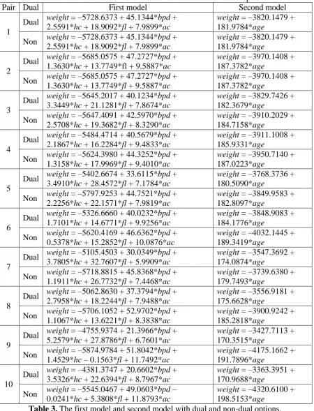
separately by equation 3 for the first model and by equation 4 for the second model. Table 3 shows the resulted first model and second model with dual and non-dual options.

Pair Dual First model Second model

1

Dual weight = –5728.6373 + 45.1344*bpd + 2.5591*hc + 18.9092*fl + 7.9899*ac

weight = –3820.1479 + 181.9784*age

Non weight = –5728.6373 + 45.1344*bpd + 2.5591*hc + 18.9092*fl + 7.9899*ac

weight = –3820.1479 + 181.9784*age

2

weight = –3970.1408 + 187.3782*age

3

weight = –3829.7426 + 182.3679*age

weight = –3910.2029 + 184.7158*age

4

weight = –3911.1008 + 185.9331*age

weight = –3950.7140 + 187.0223*age

5

weight = –3768.3736 + 180.5090*age

weight = –3849.9583 + 182.8097*age

6

weight = –3848.9083 + 184.1776*age

weight = –4032.1445 + 189.3419*age

7

weight = –3547.3692 + 174.0874*age

weight = –3739.6380 + 179.7493*age

8

weight = –3556.9181 + 175.6628*age

weight = –3900.9242 + 185.2818*age

9

weight = –3427.7113 + 170.3515*age

Non weight = –5874.9784 + 51.8042*bpd + 1.4529*hc – 0.1563*fl + 11.7492*ac

weight = –4175.1662 + 191.7896*age

10

weight = –3363.3951 + 170.9688*age

Non weight = –5545.0467 + 49.0603*bpd – 0.0241*hc + 5.3808*fl + 11.8793*ac

weight = –4320.6100 + 198.5153*age

Table 3. The first model and second model with dual and non-dual options.

When sample is complete with the 1st_{pair and the 2}nd_{pair, DREM results the same models as}

(9)

f{i}{d/n} and g{i}{d/n} be the first model and the second model with regard to the testing pair ith

and dual/non-dual option. For example, f1d is the first model derived from the 1st testing pair

with dual option whereas g2n is the second model derived from the 2nd testing pair with

non-dual option. By looking up table 3.1, we have f1d = weight = –5728.6373 + 45.1344*bpd +

2.5591*hc + 18.9092*fl + 7.9899*ac and g2n = weight = –3970.1408 + 187.3782*age.

We analyze the experimental results by two ways:

- By the first analyzed way, so-called test 1, we analyze results of REM algorithm on the first model with both dual and non-dual options. This test evaluates how good the first model is.

- By the second analyzed way, so-called test 2, we analyze results of REM algorithm on the second model with both dual and non-dual options. This test evaluates how good the second model is.

For example, given mean absolute error (MAE), by the test 1, for each case in the test dataset sample{i}.test, we compute the deviation between the weight in such case and the estimated weight resulted from the first model f{i}{d/n} in order to calculate MAE. Let U = {u1, u2,…, uK}

and V = {v1, v2,…, vK} be sets of actual weights and estimated weights, respectively. In test 1,

vi (s) are values of f{i}{d/n}. In test 2, vi (s) are values of g{i}{d/n}. Equation 9 specifies MAE

metric.

𝑀𝐴𝐸 = 1

𝐾∑|𝑣𝑖 − 𝑢𝑖|

𝐾

𝑖=1

(9)

The smaller the MAE is, the more accurate the DREM is. Table 4 shows MAE metric which evaluates our models (formulas) with test 1 and test 2.

Pair Test 1 (Dual)

Test 1 (Non-dual)

Test 2 (Dual)

Test 2 (Non-dual) 1 174.4489 174.4489 242.5407 242.5407 2 162.3012 162.3012 249.5374 249.5374 3 175.7541 174.4708 241.7887 240.8631 4 162.5601 163.0694 250.8867 250.4620 5 180.1436 175.1376 242.9584 242.3857 6 162.1598 163.8128 251.4266 250.0164 7 186.9349 177.8223 246.0096 242.8904 8 164.6054 161.9048 254.0628 249.5981 9 196.2846 173.3726 249.6362 243.6904 10 187.4117 169.2374 261.7162 255.2253 Average 175.2604 169.5578 249.0563 246.7210

Table 4. MAE of test 1 and test 2

Let rMAE{t}{i≥3}{d/n} be the bias ratio between MAE of test t and pair i with dual or non-dual

option and MAE of test t and pair 1 if i odd or pair 2 if i even. For example, we have:

𝑟𝑀𝐴𝐸_13𝑑 =175.7541 − 174.4489

174.4489 ≈ 0.0075 𝑟𝑀𝐴𝐸_24𝑛 = 250.4620 − 249.5374

249.5374 ≈ 0.0037

These bias ratios indicates withstanding of DREM for incomplete data. For instance, the value rMAE13d = 0.0075 implies that the accuracy of dual DREM decreases 0.75% when the

completion of training dataset of 3rd pair in test 1 decreases 20%. The value rMAE24n = 0.0037

implies that the accuracy of non-dual DREM decreases 0.37% when the completion of training dataset of 4th_{pair in test 2 decreases 20%. The bias ratios of test 1 and pairs 3}rd_{(20% missing}

(10)

3rd, 5th, 7th, and 9th with non-dual option are 0.51%, 0.27%, 2.4%, and 7.6%. It is concluded that such bias ratios are much smaller than percentages of missing values and so the withstanding of DREM for missing values is significant. For instance, we make a one-way paired t-test of X = {20%, 40%, 60%, 80%} and Y = {0.75%, 3.26%, 7.16%, 12.52%}. Given significant level 95%, the statistic t0 is:

𝑡₀ = 𝐷̅ 𝑠_𝐷⁄√4=

0.4408

0.2078 2⁄ ≈ 4.2433

Where,

𝐷 = 𝑋 − 𝑌 = {0.1925,0.3674,0.5284,0.6748}

Note that 𝐷̅ = 0.4408 and sD = 0.2078 are sample mean and sample standard deviation of D.

Because the t0 is larger than the percentage point t0.05, 3 = 2.353, difference between the

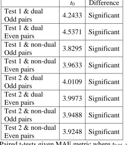
percentage of missing values and the percentage of decrease in accuracy of DREM is significant within test 1, odd pairs (3rd, 5th, 7th, 9th), and dual option. Table 5 shows paired t-tests for test 1 and test 2 with dual / non-dual options, given MAE metric and significant level 95%. We use odd pairs (even pairs) in a same group which is compared with the 1st pair (2nd pair) because odd pairs (even pairs) share the same testing dataset sample1.test (sample2.test).

t0 Difference

Test 1 & dual

Odd pairs 4.2433 Significant Test 1 & dual

Even pairs 4.5371 Significant Test 1 & non-dual

Odd pairs 3.8295 Significant Test 1 & non-dual

Even pairs 3.9633 Significant Test 2 & dual

Even pairs 3.9248 Significant

Table 5. Paired t-tests given MAE metric where t0.05, 3 = 2.353

From paired t-tests in table 5, it is asserted that the withstanding of DREM for missing values with regard to MAE metric is significant because the bias ratios with regard to MAE metric are much smaller than percentages of missing values.

We compare the mean (average) of MAE metric with regard to dual option and non-dual option. In both test 1 and test 2, DREM with dual option decreases MAE metric very little (– 5.70 ≈ 175.2604 – 169.5578 in test 1 and 2.34 ≈ 249.0563 – 246.7210 in test 2). In other words, dual DREM does not improve both the first model and the second model with subject to MAE metric. However, the deviation of MAE between test 1 and test 2 with dual option (73.7959 = 249.0563 – 175.2604) is smaller than the deviation of MAE between test 1 and test 2 with non-dual option (77.1632 = 246.7210 – 169.5578). This implies that non-dual option makes trade-off between the first model and the second model. Moreover we will know later that dual option will also increase convergence of DREM by decreasing the number of iterations.

(11)

𝑅𝑀𝑆𝐸 = √1

𝐾∑(𝑣𝑖 − 𝑢𝑖)2

𝐾

𝑖=1

(10)

The smaller the RMSE is, the more accurate the DREM is. Table 6 shows RMSE metric which evaluates our models (formulas) with test 1 and test 2.

Pair Test 1 (Dual)

Test 1 (Non-dual)

Test 2 (Dual)

Table 6. RMSE of test 1 and test 2

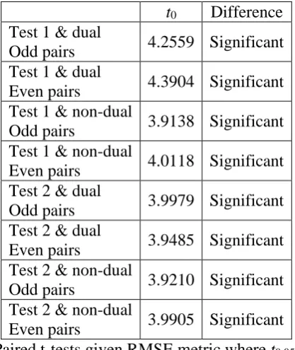
Table 7 shows paired t-tests for test 1 and test 2 with dual / non-dual options, given RMSE metric and significant level 95%.

t0 Difference

Test 1 & dual

Even pairs 3.9905 Significant

Table 7. Paired t-tests given RMSE metric where t0.05, 3 = 2.353

From paired t-tests in table 7, it is asserted that the withstanding of DREM for missing values with regard to RMSE metric is significant because the bias ratios with regard to RMSE metric are much smaller than percentages of missing values.

(12)

deviation of RMSE between test 1 and test 2 with dual option (81.7239 = 316.4258 – 234.7019) is smaller than the deviation of RMSE between test 1 and test 2 with non-dual option (87.7904 = 315.4747 – 227.6843).

We evaluate DREM with error ranges. Equation 11 specifies error range metric.

𝑑𝑖 = 𝑣𝑖 − 𝑢𝑖

𝜇 = 1 𝐾∑ 𝑑𝑖

𝐾

𝑖=1

𝜎 = √ 1

𝐾 − 1∑(𝑑𝑖 − 𝜇)2

𝐾

𝑖=1

𝑒𝑟𝑟𝑜𝑟_𝑟𝑎𝑛𝑔𝑒 = [𝜇 − 𝜎, 𝜇 + 𝜎] = 𝜇 ∓ 𝜎 = 𝜇 ± 𝜎

(11)

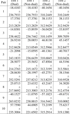
The smaller both error mean μ and error standard deviation σ are, the more accurate the DREM is. Table 8 shows error ranges which evaluate our models (formulas) with test 1 and test 2.

Pair Test 1 (Dual) Test 1 (Non-dual) Test 2 (Dual) Test 2 (Non-dual) 1 –18.4183 ± 236.7933 –18.4183 ± 236.7933 –40.1656 ± 310.2449 –40.1656 ± 310.2449 2 17.3781 ± 213.2829 17.3781 ± 213.2829 38.1153 ± 312.9429 38.1153 ± 312.9429 3 –14.8301 ± 238.4622 –15.8939 ± 236.7462 –36.0420 ± 310.1459 –33.8197 ± 309.7059 4 26.9210 ± 212.8628 28.0853 ± 213.0549 46.8130 ± 312.5966 45.1457 ± 312.8477 5 –21.2098 ± 243.1833 –15.0595 ± 236.6439 –40.1361 ± 310.6845 –40.7017 ± 310.0426 6 28.5077 ± 214.2763 25.5652 ± 215.1672 47.8504 ± 312.3195 44.5196 ± 313.5841 7 –28.0630 ± 252.5291 –28.1997 ± 237.8212 –45.2751 ± 313.8235 –38.1546 ± 310.9528 8 25.0713 ± 217.8692 23.6332 ± 213.3003 43.2167 ± 313.2176 34.3020 ± 312.4754 9 –40.1527 ± 263.0232 –11.0795 ± 238.8815 –57.1823 ± 316.5442 –49.6731 ± 310.0082 10 57.7590 ± 235.3004 44.6905 ± 221.6502 73.2199 ± 315.2914 75.6217 ± 319.1380

(13)

Because error range is not scalar, it is incorrect to make paired t-tests and so we cannot assert the withstanding of DREM for missing values with regard to error range. It is also incorrect to calculate the mean (average) of error ranges but we assert that dual DREM does not improve the first model and the second model with subject to error range because error means and error standard deviations of dual option are often larger than those of non-dual option.

We evaluate DREM with correlation coefficient (R). Equation 12 specifies R metric.

𝑅 = ∑𝐾𝑖=1(𝑢𝑖 − 𝑢̅)(𝑣𝑖− 𝑣̅) √∑𝐾𝑖=1(𝑢𝑖 − 𝑢̅)2√∑𝐾𝑖=1(𝑣𝑖− 𝑣̅)2

𝑢̅ = ∑ 𝑢_𝑖

𝐾

𝑖=1

𝑣̅ = ∑ 𝑣𝑖 𝐾

𝑖=1

(12)

The correlation coefficient R reflects adequacy of a given formula. The larger the R is, the better the formula is. Table 9 shows metric R which evaluates our models (formulas) with test 1 and test 2.

Pair Test 1 (Dual)

Test 1 (Non-dual)

Test 2 (Dual)

Table 9. R metric of test 1 and test 2

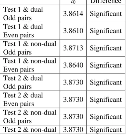
Table 10 shows paired t-tests for test 1 and test 2 with dual / non-dual options, given R metric. t0 Difference

Test 1 & dual

(14)

Even pairs

Table 10. Paired t-tests given R metric where t0.05, 3 = 2.353

From paired t-tests in table 10, it is asserted that the withstanding of DREM for missing values with regard to R metric is significant because the bias ratios with regard to R metric are much smaller than percentages of missing values.

We compare the mean (average) of R metric with regard to dual option and non-dual option. In both test 1 and test 2, DREM with dual option does not increase R. Even though, DREM with dual option almost does not changes R (–0.001 ≈ 0.9573 – 0.9584 in test 1 and 0 = 0.9198 – 0.9198 in test 2). In other words, dual DREM does not improve both the first model and the second model with subject to R metric. However, dual option makes trade-off between the first model and the second model because the deviation of R between test 1 and test 2 with dual option (0.0375 = 0.9573 – 0.9198) is smaller than the deviation of R between test 1 and test 2 with non-dual option (0.0386 = 0.9584 – 0.9198).

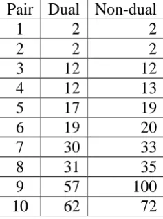
With regard to metrics such as MAE, RMSE, and R then, DREM surely withstands incomplete data. Its accuracy decreases insignificantly when the percentages of missing values increases significantly. However dual option does not improve DREM in accuracy for both the first model and the second model although duality is a feature of DREM. However, there is an interesting discovery under duality of DREM. Table 11 lists the number of iterations of DREM with regard to dual option and non-dual option.

Pair Dual Non-dual

1 2 2

2 2 2

3 12 12

4 12 13

5 17 19

6 19 20

7 30 33

8 31 35

9 57 100

10 62 72

Table 11. The number of iterations of DREM with dual / non-dual option

From table 11, the number of iterations in dual option is smaller, which means that the convergence of DREM is improved with dual option. The reason is that DREM with dual option takes advantages prior information from both the first model and the second model in order to speed up the convergence. Especially, the more the sparse ratio (percentage of missing values) increases, the more dual option brings into play. The sample in this research is not huge and so such improvement is insignificant.

An alternative technique to improve the convergence of DREM is to initialize the parameter Θ1_{= (α}1_,_β1₎T_{at the first iteration of EM process in proper way instead of initializing Θ}1_in

arbitrary way. Note, by default, Θ1 is initialized as zero vector. Let X’ be the complete matrix of ultrasound measures, which is created by removing rows whose respective weights zi (s) are

missing from X. Similarly, let Y’ be the complete matrix of fetal ages, which is created by removing rows whose respective weights zi (s) are missing from Y. Let z’ be the complete

vector of non-missing weights. The advanced Θ1 is initialized by equation 13.

{𝛼

1 _{= (𝑿}′𝑇_𝑿′₎−1_𝑿′𝑇_𝒛′

𝛽1 _{= (𝒀}′𝑇_𝒀′₎−1_𝒀′𝑇_𝒛′ (13)

(15)

z can be incomplete. Table 12 lists the number of iterations of DREM with advanced Θ1 and terminated threshold ε = 0.001.

Pair Dual Non-dual

1 1 1

2 1 1

3 7 1

4 9 1

5 14 1

6 15 1

7 23 1

8 25 1

9 42 1

10 44 1

Table 12. The number of iterations of DREM with advanced initialized parameter From comparing table 12 with table 11, it is asserted that the advanced initialized parameter Θ1_{improves the convergence of DREM. The interesting result is that non-dual option seems}

to be preeminent in speeding up DREM with advanced Θ1 whereas it is worse option with arbitrary Θ1. Now we test DREM with advanced Θ1 and very small terminated threshold ε = 10–10.

Pair Dual Non-dual

1 1 1

2 1 1

3 18 3

4 19 6

5 31 8

6 34 8

7 53 13

8 58 15

9 107 40

10 110 27

Table 13. The number of iterations of DREM with advanced initialized parameter and very small terminated threshold

From table 13, there is no doubt that non-dual option is preeminent in speeding up DREM with advanced Θ1. In general, dual option is only useful if researchers want to build up two acceptable (mutual) regression models because dual option makes trade-off between the first model and the second model. Recall that the essence of DREM is to build up two mutual regression models in duality but scientists can turn off such dual option.

4. Conclusions

(16)

can be missing. We may also introduce another algorithm different from DREM which is also another implementation of the proposal mentioned in the chapter “Phoebe Framework and Experimental Results for Estimating Fetal Age and Weight” of the book “E-Health” by Thomas F. Heston. If such hazard problem is solved successfully, practitioners will have a lot of benefits when they will not be stressful in taking ultrasound examinations because some measures are allowed to be missing. In other words, it is acceptable for practitioners to make unintentional mistakes when taking ultrasound examinations. Moreover researchers also get benefits because they can receive estimation models from incomplete sample. In literature of EM algorithm, there are methods to estimate regression model with lack of some independent variables and so the improvement of DREM is feasible.

Acknowledgements

We show our deep gratitude to Prof. Tran, Bich-Ngoc who gave us comments to evaluate the withstanding of DREM for missing values.

References

Akinola, R. A., Akinola, O. I., & Oyekan, O. O. (2009, January). Sonography in fetal birth weight estimation. Educational Research and Review, 4(1), 16-20. Retrieved from https://goo.gl/Pfjrri

Bennini, J. R., Marussi, E. F., Barini, R., Faro, C., & Peralta, C. A. (2009, December 9). Birth-weight prediction by two- and three-dimensional ultrasound imaging. Ultrasound in Obstetrics & Gynecology, 35(4), 426-433. doi:10.1002/uog.7518

Cohen, J. M., Hutcheon, J. A., Kramer, M. S., Joseph, K. S., Abenhaim, H., & Platt, R. W. (2010, April 1). Influence of ultrasound-to-delivery interval and maternal–fetal characteristics on validity of estimated fetal weight. Ultrasound in Obstetrics & Gynecology, 35(4), 434-441. doi:10.1002/uog.7506

Dempster, A. P., Laird, N. M., & Rubin, D. B. (1977). Maximum Likelihood from Incomplete Data via the EM Algorithm. (M. Stone, Ed.) Journal of the Royal Statistical Society, Series B (Methodological), 39(1), 1-38.

Deter, R. L., Rossavik, I. K., & Harrist, R. B. (1988, May 1). Development of individual growth curve standards for estimated fetal weight: I. Weight estimation procedure. Journal of Clinical Ultrasound, 16(4), 215-225. Retrieved from https://www.ncbi.nlm.nih.gov/pubmed/3152508

Eberg, M., Platt, R. W., & Filion, K. B. (2017, November 1). The Estimation of Gestational Age at Birth in Database Studies. Epidemiology, 28(6), 854-862. doi:10.1097/EDE.0000000000000713

Hadlock, F. P., Harrist, R. B., Sharman, R. S., Deter, R. L., & Park, S. K. (1985, February 1). Estimation of fetal weight with use of head, body and femur measurements: A prospective study. American Journal of Obstetrics and Gynecology, 151(3), 333-337. doi:10.1016/0002-9378(85)90298-4

Ho, T. T. (2011). Nghiên Cứu Phương Pháp Ước Lượng Trọng Lượng Thai, Tuổi Thai Bằng Siêu Âm Hai và Ba Chiều. Hanoi Univerisy of Medicine. Hanoi: Hanoi Univerisy of Medicine. Retrieved 2011

Ho, T. T., & Phan, D. T. (2011, December). Ước lượng cân nặng của thai từ 37 – 42 tuần bằng siêu âm 2 chiều. (D. Thai, Ed.) Journal of Practical Medicine, 12(797), 8-9.

(17)

Hutcheon, J. A., & Platt, R. W. (2008, April 1). The Missing Data Problem in Birth Weight Percentiles and Thresholds for "Small-for-Gestational-Age". American Journal of Epidemiology, 167(7), 786-792. doi:10.1093/aje/kwm327

Lee, W., Balasubramaniam, M., Deter, R. L., Yeo, L., Hassan, S. S., Gotsch, F., . . . Romero, R. (2009, November 1). New fetal weight estimation models using fractional limb volume. (M. A. Zoppi, Ed.) Ultrasound in Obstetrics & Gynecology, 34(5), 556-565. doi:10.1002/uog.7327

Lindsten, F., Schön, T. B., Svensson, A., & Wahlström, N. (2017). Probabilistic modeling – linear regression & Gaussian processes. Uppsala University, Department of Information Technology. Uppsala: Uppsala University. Retrieved January 24, 2018, from

http://www.it.uu.se/edu/course/homepage/sml/literature/probabilistic_modeling_comp endium.pdf

Montgomery, D. C., & Runger, G. C. (2010). Applied Statistics and Probability for Engineers (5th ed.). Hoboken, New Jersey, USA: John Wiley & Sons. Retrieved from https://books.google.com.vn/books?id=_f4KrEcNAfEC

Nguyen, L. (2015). Matrix Analysis and Calculus (1st ed.). (C. Evans, Ed.) Hanoi, Vietnam:

Lambert Academic Publishing. Retrieved from

https://www.shuyuan.sg/store/gb/book/matrix-analysis-and-calculus/isbn/978-3-659-69400-4

Nguyen, L., & Ho, H. (2014, March 30). A framework of fetal age and weight estimation. (B. S. Shetty, J. Morales, a. badawy, C. Mowa, K. K. Shukla, T. Chen, . . . G. Androutsopoulos, Eds.) Journal of Gynecology and Obstetrics (JGO), 2(2), 20-25. doi:10.11648/j.jgo.20140202.13

Phạm, T. T. (2000). Ước lượng cân nặng thai nhi qua các số đo của thai trên siêu âm. Ho Chi Minh University of Medicine and Pharmacy. Ho Chi Minh: Ho Chi Minh University of Medicine and Pharmacy.

Phan, D. T. (1985). Ứng dụng siêu âm để chẩn đoán tuổi thai và cân nặng thai trong tử cung. Hanoi University of Medicine. Hanoi: Hanoi University of Medicine.

Pinette, M. G., Pan, Y., Pinette, S. G., Blackstone, J., Garrett, J., & Cartin, A. (1999, December 1). Estimation of Fetal Weight: Mean Value from Multiple Formulas. Journal of Ultrasound in Medicine, 18(12), 813-817. Retrieved from https://www.ncbi.nlm.nih.gov/pubmed/10591444

Salomon, L. J., Bernard, J. P., & Ville, Y. (2007, May 1). Estimation of fetal weight: reference range at 20–36 weeks' gestation and comparison with actual birth-weight reference range. Ultrasound in obstetrics & gynecology, 29(5), 550-555. doi:10.1002/uog.4019 Siggelkow, W., Schmidt , M., Skala, C., Boehm, D., Forstner, S. v., Koelb, H., & Tresch, A.

(2010, February 20). A new algorithm for improving fetal weight estimation from ultrasound data at term. Archives of gynecology and obstetrics, 283(3), 469-474. doi:10.1007/s00404-010-1390-8

Varol, F., Saltik, A., Kaplan, P. B., Kilic, T., & Yardim, T. (2001, June). Evaluation of Gestational Age Based on Ultrasound Fetal Growth Measurements. (J.-W. Park, Ed.) Yonsei Medical Journal, 42(3), 299-303. doi:10.3349/ymj.2001.42.3.299