Multiple Differential Cryptanalysis using \LLR and $\chi^2$ Statistics

Multiple Differential Cryptanalysis

Using

LLR

and

χ

Statistics

C´eline Blondeau1?_{, Benoˆıt G´erard}2??_{, and Kaisa Nyberg}1

1 _{Aalto University School of Science, Department of Information and Computer}

Science 2

UCL Crypto Group, Universit´e catholique de Louvain, ICTEAM Institute

Abstract. Recent block ciphers have been designed to be resistant against differential cryptanalysis. Nevertheless it has been shown that such resistance claims may not be as accurate as wished due to recent advances in this field. One of the main improvements to differential crypt-analysis is the use of many differentials to reduce the data complexity. In this paper we propose a general model for understanding multiple differential cryptanalysis and propose new attacks based on tools used in multidimensional linear cryptanalysis (namelyLLRandχ2 statistical tests). Practical cases to evaluate different approaches for selecting and combining differentials are considered on a reduced version of the cipher PRESENT. We also consider the accuracy of the theoretical estimates corresponding to these attacks.

Keywords:block cipher, multiple differential cryptanalysis, statistical test, data complexity.

1 Introduction

Differential cryptanalysis has been introduced in 1990 by Biham and Shamir [3, 4] in order to break the Data Encryption Standard block ci-pher. This statistical cryptanalysis exploits the existence of adifferential,

i.e., a pair (α, β) of differences such that for a given input difference α, the output difference after encryption equals β with a high probability. This attack has been successfully applied to many ciphers and has been extended to various attacks, such as truncated differential cryptanalysis or impossible differential cryptanalysis, for instance.

In the original version of differential cryptanalysis [3], a unique dif-ferential is exploited. Then, Biham and Shamir improved their attack by considering several differentials having the same output difference [4].

? _{The research described in this paper by this author has been funded by the Academy}

of Finland under project 122736 and was partly supported by the European Com-mission through the ICT program under contract ICT-2007-216676 ECRYPT II.

??

Truncated differential cryptanalysis introduced by Knudsen [19] uses dif-ferentials with many output differences that are structured as a linear space. A theoretical framework have recently been proposed to analyze attacks using multiple differentials by summing the corresponding coun-ters [9]3_.

The motivation of this work is to investigate other different techniques for combining information from multiple differentials. As shown in the case of linear cryptanalysis, different approaches may be used depending on the context. In 2004, Biryukovet al.proposed a multiple linear crypt-analysis under the assumption that linear approximations are statistically independent4 _{[5]. Later Hermelin et al. introduced the multidimensional}

linear cryptanalysis [14, 15]. Contrary to previous attacks, the multidi-mensional technique focuses on the distribution of the vector of parity bits obtained when applying approximations to a single plaintext/ciphertext pair instead of considering the vector of empirical biases. In that case, the independence assumption is removed but some heuristic might be used when theoretically analyzing the attack. For both approaches, classical statistical tools are used to distinguish the statistic corresponding to the correct key guess from wrong ones. Again, the choice of the tool may depend on the context. For instance, in [10], because of the hardness of profiling the distribution corresponding to the correct key, the attack on PRESENT shows better results using χ2 _{than usingLLRstatistic.}

Our contributions.Our contributions are threefold. First, we introduce a general way of formalizing differential attacks by defining the notion of

partition functions (this corresponds to the way counters corresponding to output differences are gathered). Second, we consider the χ2 _{and the} LLRstatistical tests used in multidimensional linear cryptanalysis as tools for combining information from the groups of differentials determined by the partition function. We derive estimates for the data complexities of the corresponding differential attacks. Finally, we present a set of exper-iments that aim at (i) evaluating the accuracy of the estimates derived, (ii) comparing χ2 _{and LLR combining tools and (iii) comparing different}

partition functions.

The paper is organized as follows. In Section 2 we define the nota-tions and recall some results from order statistics that will be used to

3 _{In [1], in parallel to this work, the authors perform an attack on a reduced}

ver-sion of KATAN32 using the LLR statistical test. Estimate of the output difference distribution is then done by enciphering the full codebook for different keys. 4

derive data complexity estimates. Further, in Section 3 we present a gen-eral model for multiple differential cryptanalysis, introduce the notion of

partition function and link this notion with already published differential attacks. Then, in Section 4, we present two tools for combining informa-tion based on theLLRand theχ2_{statistical tests. We derive estimates for}

the corresponding data complexities and also discuss the way of choosing

partition functions. Finally, Section 5 contains the experiments that have been performed to compare the different methods.

2 Theoretical Background

2.1 Differential Cryptanalysis Against SPN Ciphers

In this paper we consider SPN ciphers that form a subclass of iterated block ciphers. Let m be the block size of the considered cipher E and

K the key used for enciphering samples: E : Fm2 −→ Fm2 , x 7→ EK(x).

Then, sinceE is an iterated block cipher, it can be expressed asEK(x) =

FKr◦ · · · ◦FK1(x),whereF is the round function parameterized by round

sub-keysK1, . . . , Kr.

The attack we are interested in is a member of the so-called last-round attacks, which themselves constitute the major part of statisti-cal cryptanalyses. These last-round5 _{attacks use a particular behavior of}

FKr−1◦· · ·◦FK1 (that is often referred asstatistical characteristic) to

par-tially recover the value of Kr. In the following we will use the compact

notationFr0 K

def

= FK_r0 ◦ · · · ◦FK1. The idea is to partially decipher

cipher-texts using different values for a part ofKr that we namecandidates and

denote by k. In the case of an incorrect guess we obtain outputs corre-sponding toF_k−1◦Fr

K while for the correct key guessk0 the outputs

corre-spond toF_Kr−1 and thus the statistical characteristic should be observed if enough samples are available. Such attack relies on the assumption that

F_Kr−1can be distinguished from the set of functionsF_k−1◦Fr

K. In practical

situations, the latter functions behave as randomly chosen permutations as stated by the following Wrong Key Randomization Hypothesis.

Hypothesis 1 (Wrong Key Randomization) Functions F_k−1 ◦Fr K for wrong key candidates k are indistinguishable from randomly chosen per-mutations.

5

Assuming that this hypothesis does not hold would mean thatr+ 1 rounds of the cipher are distinguishable and hence the attacker should be able to attack more rounds. As a consequence, this hypothesis is quite reasonable as soon as the attacker targets the largest number of rounds he is able to attack (which is typically the case). The resulting attack consists of the following three steps.

1 Distillation. For each key candidate ciphertexts are partially deci-phered. The number of occurrences of the characteristic is stored for each candidate.

2 Analysis.Key candidates are ranked according to the counters com-puted in the Distillation step.

3 Search.Finally, all master keys corresponding to the most likely key candidate are exhaustively tested. If the correct master key is not found then the search step is performed again using the second most likely candidate and so on . . .

Differential cryptanalysis. Here we consider the basic differential crypt-analysis which is a last-round attack where the statistical characteristic is an (r−1)-round differential. It is a pair of input/output differences (δ0, δr−1) and the corresponding probability p(δ0 →δr−1),

p(δ0→δr−1) def

= PrX,K

F_K−_r1(EK(X))⊕F_K−_r1(EK(X⊕δ0)) =δr−1

.

Usually, it is assumed that for an incorrect key candidate the probabil-ity of observing the differential is 1

2m₋₁. Nevertheless, it has been recalled in [12] that considering thatF_k−1◦Fr

K acts as a random permutation, the

distribution of this probability is known to be a Poisson distribution with parameter 1

2m₋₁.

Using more than one characteristic. Using many characteristics allows the attacker to extract more information from available samples what is of interest as soon as the induced overhead (in both distillation and analysis steps) is negligible compared to the gain in the final search step induced by the additional information obtained (due to the better rank-ing of the correct key). Premise of this approach have already been pro-posed in some papers by independently considering different differentials [4] (different analysis phases for different characterics) or by summing the information coming from the different characterics to perform all in one step. In the context of linear cryptanalysis, the method known as

candidate. While the question of characteristics combination have been deeply studied for linear cryptanalysis [18, 5, 13–15], the lack of a com-prehensive study on this topic in the context of differential cryptanalysis motivates the present work. In the following, and after presenting the required background, we propose a general framework and instantiate it with statistical tools already shown to be useful for linear cryptanalysis. Later on, we present experiments we ran to determine what seems to be the best combining technique in practice.

2.2 Order statistics for Gaussian variables

We propose here to recall a result on order statistics for normally dis-tributed random variables that have been used by Sel¸cuk to derive esti-mates of the data complexity for single linear6 _{cryptanalysis [22]. Let us}

model the attack as follows. We will see later that, due to the tools used, scores obtained will fit into this model.

Model 1 Let S(k) be the score/statistic obtained for a key candidate k. Then,

S(k)∼

N(µR, σ2_R), ifk=k0,

N(µW, σW2 ),otherwise.

Assuming that this model holds then the distributions of ordered wrong-key scores are also normally distributed. This allows expressing the num-ber of required samples for the attack as a function of the minimum rank wished for the correct key and the probability of this rank to be reached. Works have shown that the data complexity of an attack is not influenced by nbut by its advantage a[22, 8] that we define now.

Definition 1. Let 2n _{be the number of possible key candidates and ` the} maximum number of candidates that will be considered in the final search step. Then, the advantage of such attack over exhaustive search is defined as:

adef= n−log₂(`).

The success probability of an attack Ps is the probability that the correct key candidate is ranked among the ` first candidates at the output of analysis step.

6

The following result expresses the success probability of an attack in the Model 1 as a function of the parameters µR, σR, µW and σW. This

result is the cornerstone of further data complexity estimate derivations.

Lemma 1. Let a be the advantage of an attack and Ns be the number of available samples, then, the success probability of the attack PS can be approximated by:

PS≈Φ0,1 



µR−µa q

σ2 a+σR2



,

where µa=µW +σWΦ₀−_,1₁(1−2−a), and,σ2a≈ σ2

W2

−(n+a) ϕ2

0,1(Φ

−1

0,1(1−2−a)) .

Proof. The proof follows the one of Theorem 1 in [22].

Remark. For the different applications considered in this paper,σaturns

out to be negligible compared to σr and hence we will consider that

σ2

a+σR2 =σ2R. Indeed, it can be proved7 that 2 −(n+a) ϕ2

0,1(Φ

−1

0,1(1−2−a)) ≈ _√2−n

2π. In

typical cases,nwill be large enough for σ2

a to be small compared toσ2W.

Since in the worst observed case,σ2

R≈σ2W, thenσa2will also be negligible

compared to σ2

R. Hence, we will use the following approximation for Ps:

PS =Φ0,1

µR−µW −σWΦ−0,11(1−2−a)

σR

!

. (1)

We will discuss this last point later in the respective sections and provide observed values.

3 General Model for Multiple Differential Cryptanalysis

In simple differential cryptanalysis, one sample is composed of a pair of

plaintexts (x, x⊕δ0) and the corresponding ciphertexts (y=EK(x), y0 =Ek(x⊕δ0)).

Eventually, multiple input differences may be used to perform an attack and then structures should be use to generate more samples from less plaintexts. In the following, we will study the complexities of different at-tacks in terms of the numberNsof required samples to avoid ambiguities.

In the case where a single input difference is used then the corresponding data complexity N will be N = 2Ns. If more than one input difference

is used, then plaintexts should be grouped into structures and then the coefficient 2 in the data complexity may change.

7

3.1 Partition in differential cryptanalysis

In this section, we propose a general model for multiple differential crypt-analysis. The aim of such a model is to provide a common language to express various notions of differential cryptanalysis (multiple, improba-ble, impossiimproba-ble, . . . ) in such a way that the same analysis tools can be used to evaluate performance of the attacks. This model will also help in the investigation for new techniques that handle multiple characteristics. From a very abstract point of view, a differential cryptanalysis is com-posed of two functions.

– First a sampling function processes, for each key candidate k, the

Ns available samples (si)1≤i≤Ns and extracts the corresponding dif-ference distributions qk _{by normalizing the counters. This function}

corresponds to the distillation step.

η : FN₂2sm× K →[0,1]2 m

, {s1, . . . , sNs}, k

7→qk_{= (q}k δ)δ∈_F2m where

qk δ =

1

Ns

#

si = (yi, y0i), Fk−1(yi)⊕F

−1 k (y

0

i) =δ .

– Second, a scoring function extract a score for the candidate k from the empirical distribution qk _{of observed differences. This function}

corresponds to the first part of the analysis step (then candidates are ordered from the most likely to the least one).

ψ: [0,1]2m →R, qk7→ψ(qk).

Since in actual ciphersm ≥64, the storage of distributions qk _{is not}

possible. The solution is to consider smaller distributions. From a general point of view, this can be done by projecting the observed differences on a set of smaller cardinality by partitioning the space of output differences. We will show later how known attacks translate into this model. We denote byπ such partition function fromF2m to a setV (we assume that

V = Im(π)). We can generalize the sampling and scoring functions by considering the partition functionπ.

Model 2 In differential cryptanalysis, the score of a key candidate is ob-tained composing the following two functions defined for a given mapping π from F2m to a setV.

ηπ : FN₂2sm× K →[0,1]

|V|

, {s1, . . . , sNs}, k

where

qk_v def= 1

Ns

#

si= (yi, yi0), π F

−1

k (yi)⊕F

−1 k (y

0

i)

=v ,

and

ψπ : [0,1]|V|→R, qk7→ψπ(qk).

Scoring functions and difference distributions. Later in Section 4,we will instantiate different scoring functions ψπ. Some of them are based on the

knowledge of the theoretical behavior of difference distributionsqk_{. This}

behavior obviously depends on whether kcorresponds to the correct key or not. If yes, the distributionqk _{will be determined by differential}

prob-abilities, while if not, Hypothesis 1 implies that qk _{follows a distribution}

corresponding to what would be obtained when considering the output of a random permutation. Hence, we place ourselves in the following model.

Model 3 Letkbe a subkey candidate andqk _{the corresponding difference} distribution obtained by a sampling function ηπ. Then,

Prhqk_v =xi=

Pr [pv =x],ifk=k0,

Pr [θv =x],otherwise,

where distributions p and θ are defined as

pv = X

d∈π−1_(v)

p(δ0→d) and θv =

1 #π−1_(v).

Remark. An attack based on partitioning input and output spaces was proposed by Harpes and Cramer in [17]. We would like to stress that such attack uses a partition of the plaintext (ciphertext,resp.) space while we consider in this paper partitions of input (output,resp.) difference space.

3.2 Partitions and Actual Attacks

Simple/Impossible/Improbable Differential Attacks. In these attacks, one considers a single differential (δ0, δr−1) having an unexected behavior (eg.

a too large or too small probability of occurring). Such cryptanalyses can be represented in our model using the following function identifying differences to the set indexed by V ={0,1}.

π(d) =

1,ifd=δr−1,

0,otherwise.

The corresponding scoring function is determined by the number of times the characteristic occurred hence only takes into consideration the value

Truncated Differential Attacks. Truncated differential cryptanalysis [19] is similar to differential cryptanalysis in the sense that usually only one truncated differential characteristic (∆0, ∆r−1) is used. Such attacks can

be represented in our model in the same way that the previous ones i.e.

using the projected spaceV ={0,1} and a similar partition function

π(d) =

1,ifd∈∆r−1,

0,otherwise.

Again, the corresponding scoring function only takes into consideration the value q1 of the projected distribution.

Multiple Differential Attacks. To improve the performances of differential attacks, information coming from different differentials may be combined. We consider here attacks such that differentials used have the same in-put difference. We discuss at the end of Section 5 how our model can be extended to the use of multiple input differences. Assuming that the col-lection of differentialδ0, δ(ri−)1

i=1,...,A is used, we model the attack with

projected spaceV ={0,1, . . . , A}and partition function:

π(d) =

(

i, ifd=δ(_ri₋)₁,

0,otherwise.

4 Instantiations and Complexity Estimates

In this section, we provide instantiations of scoring functions and the corresponding estimates for data complexities. Later, in Section 5 we ex-periment these scoring functions using different partition functions by attacking a reduced version of PRESENT [6, 20] and discuss the corre-sponding time and memory complexities.

4.1 The Sum-of-counters Scoring Function

This technique consists in summing counters corresponding to considered differentials. Theoretical analysis of this method is done in [9]. Taking notations of the previous section, the scoring function is determined by

PA

i=1qi or equivalently by the value 1 −q0. In this setting the scores

4.2 The LLR Scoring Function

The Neyman-Pearson lemma [21] gives the optimal form of the acceptance region on which is derived theLLRmethod. The optimality requires that both pand θ distributions are known (or at least the valuespv/θv).

Definition 2. Let p = [pv]v∈V be the expected probability distribution vector, θ the uniform one and qk _{the observed one for a key candidate k.} For a given number of sample Ns, the optimal statistical test consists in comparing the following statistic to a fixed threshold.

LLR(qk, p, θ)def= Ns X

v∈V

qvlog

pv

θv

.

An important remark here is that, similarly to the case presented in Section 4.1, theLLRstatistic can be computed with a memory complexity of one floating-point counter per candidate. Indeed, this statistic is a weighted sum of counters for which weights are known before attacking. This test has been applied in [2] by Baign`eres et al. in the case of linear cryptanalysis. Applying the law of large numbers, they shown that the

LLR statistic tends toward a Gaussian distribution with different means and variances according to the distribution q is extracted from. These means are expressed in terms of relative entropy.

Definition 3. Letpandp0 be two probability distribution vectors overV. Therelative entropy (aka.Kullback-Leibler divergence) betweenp andp0

is

D p||p0def

= X

v∈V

pvlog

pv

p0

v

.

We also define the following metrics

D2 p||p0 def

= X

v∈V

pvlog2

pv

p0

v

, and ∆D p||p0def

= D2 p||p0

−D p||p02.

Lemma 2. (Proposition 3 in [2]) The distributions ofLLR(qk_{, p, θ)} asymp-totically tend toward a Gaussian distribution as the number of samples Ns increases. If samples are obtained from distribution p (θ, resp.), the LLR statistic tends toward N(µR, σ2R) (N(µW, σW2 ), resp.), where

µR=NsD(p||θ), µW =−NsD(θ||p),

σ2

Then, we can use Lemma 1 to obtain the following result.

Theorem 1. Let abe the advantage of an attack then the number Ns of samples required to reach success probability PS is

Ns= h_p

∆D(p||θ)Φ−_0,1₁(PS) + p

∆D(θ||p)Φ₀−_,1₁(1−2−a₎i2

[D(p||θ) +D(θ||p)]2 . (2)

Proof. The proof is based on Lemma 1 and can be found in Appendix A.1.

4.3 The χ2 Scoring Function

The aforementionedLLRtest is optimal when both distributions are known. In our context, the knowledge ofθrelies on Hypothesis 1 and the knowl-edge of p is based on the possibility of the attacker to theoretically com-pute differential probabilities. Hence, the use of an alternative statistic may be of interest when one of these two distributions is unknown to the attacker. Theχ2 _{method has already proved out to be useful particularly}

in the context of linear cryptanalysis, where the correct-guess distribu-tions vary a lot with the key [10].Also in the differential case, obtaining a good estimate of the correct-guess distribution may be impossible. The idea is then to compare the empirical distribution to the wrong-guess dis-tribution: the vector corresponding to the correct key-guess should end up with one of the largest scores (i.e., the smallest probability of being drawn fromθ).

Definition 4. Letqk_{be an empirical distribution vector. Theχ}2 _statistic

used to determine the probability of the vector to correspond to a realiza-tion from distriburealiza-tion θ is

χ2_(qk_{, θ) =N} s

X

v∈V

(qk v −θv)2

θv

.

Notice that using χ2 _{method, all the counters should be stored since}

it is not possible to compute the statistic on-the-fly as it was the case when summing counters or forLLR. This results in an increased memory cost when using this technique. The following quantity appears when considering the parameters of theχ2 _{score distributions.}

C(p)def= P v∈V

(pv−θv)2

θv

.

Lemma 3. [16] The distribution ofχ2_(qk_{, θ)asymptotically tends toward} a Gaussian distribution as the numberNs of samples increases. If samples are obtained from distribution p (θ, resp.), the χ2 _{statistic tends toward}

N(µR, σR2) (N(µW, σ2W), resp.) where,

µR=|V|+NsC(p) , µW =|V|,

σ_R2 = 2|V|+ 4NsC(p) , σ2W = 2|V|.

In [16], Hermelinet al. proposed an approximation of the data com-plexity of a χ2 _{statistical test. It turns out that, at least in the present}

context, the estimate proposed in the following theorem is tighter.

Theorem 2. LetC(p)be the capacity of the correct-candidate probability vectorp. Then, the numberNs of samples of the corresponding attack with success probability PS and advantage a can be estimated by

Ns= p

2|V|b+ 2t2_+t(p

2|V|+ 2b)

r

1 + 4 t2−b2

(√2|V|+2b)2

C(p) , (3)

where b=Φ−_0,1₁(1−2−a_{) and t =Φ}−1

0,1(PS). Fixing the success probability to 0.5, we obtain the following estimate for the number of samples:

Ns= p

2|V|Φ−_0,1₁(1−2−a₎

C(p) . (4)

Proof. The proof is based on Lemma 1 and can be found in Appendix A.2.

4.4 Different Partition Functions

We present here two different types of partition functions. The first one encompass all previously proposed attacks by projecting some considered differences to corresponding elements of V and all others to 0. The sec-ond family of partition functions induce a balanced partitioning of the difference space (the sets of differences that are projected to elements of

techniques for building partition functions as respectively balanced and

unbalanced partitioning.

Let us recall that we consider that differentials used all have the same input difference, we will explain later how different input differences can be handled.

Unbalanced Partitioning When the attacker knows the probability of some differentials (δ0, δr(i−)1)1≤i≤A, then the natural way of partitioning

is to allocate a counter to each of these differentials. A “trash” counter will gather all other output differences.

πunbal(d) =

i, ifd=δi,

0,otherwise. (5)

Let us denote by∆r−1 the set of output differences∆r−1 def

= (δ_r(i₋)₁)1≤i≤A.

It is likely that this set allows early discarding of the so-called wrong pairs,i.e., pairs (y, y0_{) such that, for all candidatesk,F}−1

k (y)⊕F

−1 k (y0)6∈

∆r−1. Using such sieving process allows to decrease the number of partial

decryptions in the attack and typically results in considering active bits in the difference y⊕y0. In our model such wrong pairs will only account for the counters qk

0. As

P|V|−1

v=0 qvk= 1 (|V|=A+ 1), for each candidate

k,qk

0 can be derived from the other values. The theoretical probabilityθ0

is equal to θ0 = 1−P

|V|−1

v=1 θv= 1−

|V|−1 2m₋₁

Balanced Partitioning This alternative results in a balanced partitioning of the space of differences and hence the sieving process will not be as effective as in the case of unbalanced partitioning (if needed at all). Bal-anced partition functions consider in the experiments have a particular structure linked to truncated differentials. A supportsto indicate the set of targeted difference bits, s⊂ {0, m−1}, is determined (|V|= 2|s|_{) and}

the partition function consists of considering only bits belonging to this support:

πbal(d) =d|s=

|s|

X

i=0

2i_·d

s(i), (6)

wheres(i) denote the i-th bit that belong to the support.

all v∈V:θv = 2

m

|V|.

The main drawback of this model is that the differentials are grouped, and depending on the way this is done, the attack may be more or less efficient.

5 Experiments

In this section, we experiment different combinations of partition and

scoring functions on nine rounds of SMALLPRESENT-[8]8 _a

reduced-version of PRESENT presented in [20]. The goal is to investigate the potential improvements mentioned in Section 4 and to test their robust-ness in a real attack context (that is with potentially badly estimated distributions). More details about the choices of experiment parameters can be found in Appendix A.3.

5.1 On the Choice of Partition Functions

Depending on the targeted cipher, the structure of the possible partition functions may differ a lot. Nevertheless, using both a balanced and an

unbalanced partitioning, (see Equations (6), and (5)) we expect to cover a large spectrum of attack possibilities in the context of SPN ciphers.

About πunbal. Such unbalanced partition function is generally chosen in

such a way that an efficient sieve can be performed to discard wrong pairs. In our settings, see Equation (5) , the discarded pairs correspond to the ones that increment counter q0 for all key candidates. The use of such

sieving process leads to an important gain in the time complexity of the partial decryption phase.

The weakness of this kind of partition function is that only few pairs are really useful to the attack (non-discarded pairs). More precisely, for

Ns samples and a given index value v6= 0,

#

(y, y0)|πunbal F_k−1(y)⊕F_k−1(y0)

=v =O Ns

2m

, where Ns

2m ≤1. In the context of classical simple differential cryptanalysis this phenomenon is related to the thresholds that can be observed on curves representing success rate or advantage as a function of the number of available sam-ples. When using scoring techniques as the one proposed in this paper, this may explain part of the discrepancies between theoretical and em-pirical results, particularly in the context of χ2_.

8

Aboutπbal. In the case ofbalancedpartition functions, the aforementioned

behavior is not observed since all pairs are taken into account. Indeed,

#

(y, y0)|πbal Fk−1(y)⊕F

−1 k (y

0

)

=v =O(Ns·θv), while θv =

1

|V|.

That means that forbalancedpartition functions, ifNsis larger than|V|,

the noise is reduced9_{. Nevertheless, in such context we generally cannot}

use an efficient sieving process hence the time complexity of the resulting attack is more important: for each sample a partial decryption of the last round has to be performed. Part of this drawback is removed due to the smaller data complexity. Hence both approaches may be of interest depending on the context.

5.2 Experimental Results

The present work proposes to model multiple differential cryptanalysis as the combination of a partition and a scoring function. We derived esti-mates for the data complexity corresponding to different scoring functions and introduced two families of partition functions. Hence, there are many things that experiments may tell us about the relevance of these tools. We will first discuss the accuracy of the estimates for the data complexity we derived. Then, we will focus on the scoring functions and their robustness regarding badly estimated distributions. Thus, we ran experiments in two different contexts:

(i) using “actual” correct-key distribution: this distribution was obtained by experimentally computing differential probabilities for fixed keys and then averaging over 200 different keys10_;

(ii) using estimated correct-key distribution: we model the fact that an attacker may only have access to estimates of the differential prob-abilities by degrading the actual correct-key distribution for a given error rate.

All experiments have been performed targeting nine rounds of the cipher. The main reason is that the corresponding data complexities are high enough for the attack to make sense and small enough for us to perform enough experiments. For the same reason, we choose size of output spaces

|V|in such a way that the counter storage of the resulting attacks can be handled in RAM and that the number of key candidates is at most 216_.

9

Intuitively: for a fixed value of|V|, the noise is decreasing as the number of sample is increasing

10

Accuracy of the data complexity estimates. Accuracy of the data complexity estimates presented in Theorem 1 and Theorem 2 depends on different parameters (the size of the output space, the partition function and so on). It also strongly depends on the correctness of estimates used for the distributions. In order to focus on the validity of provided formulas, we ran experiments in the setting (i)11 _{correct-key distribution thus any}

observed deviation should not be attributed to an incorrect estimate of the differential probabilities.

0.5 0.6 0.7 0.8 0.9

20 22 24 26

PS

log2(N)

Ex.a= 4 Th.a= 4 Ex.a= 7 Th.a= 7 Set size 28

0.5 0.6 0.7 0.8 0.9

20 22 24 26

log2(N) Set size 212

Fig. 1.Data complexities of attacks usingχ2_{scoring and balanced partitioning.}

0.5 0.6 0.7 0.8 0.9

17 19 21 23

PS

log2(N)

Ex.a= 4 Th.a= 4 Ex.a= 7 Th.a= 7 Set size 28

0.5 0.6 0.7 0.8 0.9

17 19 21 23

log2(N) Set size 212

Fig. 2.Data complexities of attacks usingLLRscoring and balanced partitioning.

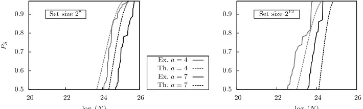
We observe that for bothχ2 _{(Figure 1) and}

LLR(Figure 2), formulas

provided by Theorem 2 and Theorem 1 give rather good estimates for the data complexity.

11

Comparison of scoring functions (known distributions). We now consider Figure 1 and Figure 2 in a different way, since we aim at compar-ing bothχ2_{andLLRscoring functions. Obviously theLLRscoring function}

has much smaller data requirement. For instance, for an advantagea= 7 and an output space size |V| = 212_{, it only requires 2}18.7 _{plaintexts to}

reach a success probability of one half while 223.55 _{is required using χ}2_.

This is a natural result since LLR attacks are run with actual values of

the differential probabilities and hence have more information to process the available data.

Comparison of scoring functions (estimated distributions). In [10], Cho has shown that if the attacker only has a badly estimated correct-key distribution then using theLLRstatistical test is not relevant

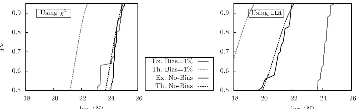
anymore. We conducted experiments in that direction assuming that the estimated probability distributions were biased. We emulated this phe-nomenon by adding some random noise to the distribution estimate (that is ˆpv =pv±₁₀₀pv) then normalizing ˆpv.

We present in Figure 3 the results of our investigation in the case of a balancedpartition function with |V|= 28 _{(case were the best match is}

obtained between theory and practice) when the attacker only knows a correct estimate of the distribution. Using both LLR or χ2 _scoring

func-tions leads to inaccurate estimafunc-tions of the data complexity.

0.5 0.6 0.7 0.8 0.9

18 20 22 24 26

PS

log2(N)

Ex. Bias=1% Th. Bias=1% Ex. No-Bias Th. No-Bias Usingχ2

0.5 0.6 0.7 0.8 0.9

18 20 22 24 26

log2(N) UsingLLR

Fig. 3.Data complexities for biased distribution (using balanced partitioning of a set of cardinality|V|= 28 with advantagea= 4).

It turns out that the noised distribution we obtained can be distin-guished from the corresponding uniform distribution θ more easily and hence theoretical expectations are optimistic. For χ2 _{method, it can be}

looking at the relative entropy betweenθand the noised distribution (that is larger). The main information is that this badly estimated distribution does not affect the attack usingχ2 _{scoring function, what is quite natural}

since the distribution pis not involved in the process, while forLLR

scor-ing function this induces an overhead in the data complexity. With only a 1% bias, χ2 _{scoring function achieve slightly better performance than} LLR(in terms of data complexity).

Notice that in practice, when instantiating attacks on real ciphers with large state size, it is not so easy to obtain a good estimation of the correct-key distributions. A folklore result is that the differential prob-ability can be underestimated by adding probabilities of corresponding differential trails found using a Branch-and-Bound algorithm. The main difficulty comes from the choice made by designers known as “wide trail strategy” [11]. Such strategy implies that the number of significant trails in a differential (or linear approximation) exponentially increases with the number of rounds. Experiments made (but not presented in this paper) show that even on SMALLPRESENT-[8] estimating distributions directly using a Branch-and-Bound algorithm leads to an error drastically larger than 1%. Hence in practice, an attacker may favor theχ2 _{scoring function.}

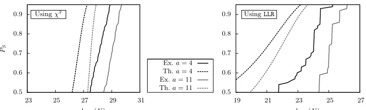
Comparing partition functions. Let us now consider the impact of partition functions used. Figure 1 and Figure 2 are related to experiments that have been performed using the newly introduced balanced partition-ing. We also ran experiments using the former unbalanced partitioning for which an efficient sieving process can be performed (see Figure 4). We chose to perform attacks with an output set of size |V| = 216_{. The}

reason is that for smaller sizes corresponding attacks require much more data. Hence, to fairly compare partition functions we used best possible parameters that allow performing enough attacks for plotting results in a given time.

0.5 0.6 0.7 0.8 0.9

23 25 27 29 31

PS

log2(N)

Ex.a= 4 Th.a= 4 Ex.a= 11 Th.a= 11 Usingχ2

0.5 0.6 0.7 0.8 0.9

19 21 23 25 27

log2(N) UsingLLR

Fig. 4.Data complexities for an unbalanced partitioning (set of cardinality 216).

On the use of differentials with different input differences. There are two straightforward ways of extending this work to multiple input differences. The first one is to consider the same partition function for each input difference so that only one output distribution is considered. The second technique is orthogonal since it consists in considering inde-pendently the distributions coming from different input differences. The corresponding scoring functions boils down to summing scores obtain for each distribution.

We ran experiments using both approaches and surprisingly did not obtained radically better results than using a single input difference. Nev-ertheless, we observed a strong correlation between the distributions ob-tained that should be exploited. This is a very promising scope for further improvements of this work.

6 Conclusion

This paper builds on the work made on the topic of linear cryptanalysis using multiple approximations. We investigate different statistical tests (namely LLRand χ2) to combine information coming from a large

num-ber of differentials while, to our knowledge, only summing counters was considered up to now. To analyze these tools, we introduce a formal way of representing multiple differential cryptanalysis using partition functions and present two different families of such functions namely balanced and

unbalanced partitioning (previous attacks being modelled as unbalanced partitioning). Finally, we present experiments performed on a reduced version of PRESENT that confirm the accuracy of the data complexity estimates derived in some contexts. These experiments show a relatively good accuracy of the estimates and illustrate the fact that usingbalanced

Further research include exploiting the similarities observed between distributions corresponding to different input differences and solving the challenging problem of estimating correct-key distributions for actual ci-phers.

References

1. Albrecht, M., Leander, G.: Private communication May, 2011

2. Baign`eres, T., Junod, P., Vaudenay, S.: How far can we go beyond linear cryptanal-ysis? In Lee, P.J., ed.:Advances in Cryptology - ASIACRYPT 2004.Volume 3329 ofLNCS., Springer (2004) 432–450

3. Biham, E., Shamir, A.: Differential cryptanalysis of DES-like cryptosystems. In Menezes, A., Vanstone, S.A., eds.:Advances in Cryptology - CRYPTO 1990.Volume 537 ofLNCS., Springer (1991) 2–21

4. Biham, E., Shamir, A.: Differential cryptanalysis of DES-like cryptosystems. Jour-nal of Cryptology4(1991) 3–72

5. Biryukov, A., Canni`ere, C., Quisquater, M.: On Multiple Linear Approximations. In: CRYPTO’04. Volume 3152 ofLNCS., Springer–Verlag (2004) 1–22

6. Bogdanov, A., Knudsen, L.R., Leander, G., Paar, C., Poschmann, A., Robshaw, M.J.B., Seurin, Y., Vikkelsoe, C.: PRESENT: An ultra-lightweight block cipher. In Paillier, P., Verbauwhede, I., eds.:Cryptographic Hardware and Embedded Systems - CHES 2007.Volume 4727 ofLNCS., Springer (2007) 450–466

7. Blondeau, C., G´erard, B.: Links between theoretical and effective dif-ferential probabilities: Experiments on PRESENT. In: TOOLS’10. (2010) http://eprint.iacr.org/2010/261.

8. Blondeau, C., G´erard, B., Tillich, J.-P.: Accurate estimates of the data complexity and success probability for various cryptanalyses. In Charpin, P., Kholosha, S., Rosnes E., and Parker, M.G. eds.: Designs, Codes and Cryptography. Volume 59 Numbers 1-3, Springer (2011) 3–34

9. Blondeau, C., G´erard, B.: Multiple Differential Cryptanalysis: Theory and Practice. In Joux, A., ed.: Fast Software Encryption - FSE 2011. Volume 6733 of LNCS., Springer (2011) 35 – 54

10. Cho, J.Y.: Linear cryptanalysis of reduced-round PRESENT. In Pieprzyk, J., ed.:Topics in Cryptology - CT-RSA 2010.Volume 5985 ofLNCS., Springer (2010) 302–317

11. Daemen, J., Rijmen, V.: The Wide Trail Design Strategy. In Honary, B., ed.:

Cryptography and Coding - IMACC 2001.Volume 2260 ofLNCS., Springer (2001) 222–238

12. Daemen, J., Rijmen, V.: Probability distributions of correlation and differentials in block ciphers. Journal of Mathematical Cryptology1(2007) 12–35

13. G´erard, B., Tillich, J.-P.: On linear cryptanalysis with many linear approximations. In Parker, M. G., ed.: Cryptography and Coding - IMACC 2009.Volume 5921 of

LNCS., Springer (2009) 112–132

15. Hermelin, M., Cho, J.Y., Nyberg, K.: Multidimensional linear cryptanalysis of reduced round Serpent. In Yi Mu, Willy Susilo, and Jennifer Seberry, ed.: Informa-tion Security and Privacy - ACISP 2008, volume 5107 of LNCS., Springer (2008) 203–215

16. Hermelin, M., Cho, J.Y., Nyberg.,K.: Multidimensional extension of Matsui’s al-gorithm 2. In Orr Dunkelman, ed.:Fast Software Encryption - FSE 2009, volume 5665 ofLNCS., Springer (2009) 209–227

17. Harpes, C., Massey, J.L.: Partitioning Cryptanalysis. In Biham, ed.:Fast Software Encryption - FSE 1997.Volume 1267 ofLNCS., Springer (1997) 13–27

18. Kaliski, B.S., Robshaw, M.J.B.: Linear Cryptanalysis Using Multiple Approx-imations. In: Advances in Cryptology - CRYPTO 1994. Volume 839 of LNCS., Springer–Verlag (1994) 26–39

19. Knudsen, L.R.: Truncated and higher order differentials. In Preneel, ed.: Fast Software Encryption - FSE 1994.Volume 1008 ofLNCS., Springer (1995) 196–211 20. Leander, G.: Small scale variants of the block cipher PRESENT. Cryptology

ePrint Archive, Report 2010/143 (2010) http://eprint.iacr.org/2010/143.

21. Neyman, P., Pearson, E.: On the problem of the most efficient tests of statistical hypotheses. Philosophical Trans. of the Royal Society of London (1933) 289–337 22. Sel¸cuk, A.A.: On probability of success in linear and differential cryptanalysis.

Journal of Cryptology21(2008) 131–147

23. Wang, M.: Differential cryptanalysis of reduced-round PRESENT. In Vaudenay, S., ed.: Progress in Cryptology - AFRICACRYPT 2008. Volume 5023 of LNCS., Springer (2008) 40–49

A Proofs

A.1 Proof of Theorem 1

We applied the result of the Lemma 1 to the LLR case. As previously mentioned12_{, we consider that σ}2

R σ2a and hence we neglect the term

σ2

a to obtain the approximation of PS given in (1)

PS=Φ0,1

µR−µW −σWΦ−_0,1₁(1−2−a)

σR

!

,

Φ−_0,1₁(PS) =

Ns[D(p||θ) +D(θ||p)]−σW Φ−0,11(1−2−a)

σR

,

p

Ns= p

∆D(p||θ)Φ−_0,1₁(PS) + p

∆D(θ||p)Φ₀−_,1₁(1−2−a₎

D(p||θ) +D(θ||p) .

What finally yields (2) and finishes the proof.

12

In Section 2 we promised figures to illustrate the fact thatσR2 σ

2

a. For instance,

A.2 Proof of Theorem 2

From Lemma 1 and assuming13 _σ2

aσR2, we can use (1)

PS =Φ0,1

µR−µW −σWΦ−0,11(1−2−a)

σR

!

.

Hence,

Φ−1_(P S) =

NsC(p)− p

2|V|Φ−_0,1₁(1−2−a₎ p

2|V|+ 4NsC(p)

.

We observe that the number of samples appears together with the capacity C(p). Let us denote by X the value NsC(p) and express this

equation as a degree-two polynomial then solve it. To lighten notation we denote Φ−1

0,1(1−2−a) byb and Φ

−1

0,1(PS) byt:

X−p

2|V|b

p

2|V|+ 4X =t,

X2_−2Xp

2|V|b+ 2|V|b2

2|V|+ 4X =t

2_,

X2_−2Xp

2|V|b+ 2|V|b2_−t2_{(2|V|+ 4X) = 0,}

X2−2X(p2|V|b+ 2t2) + 2|V|(b2−t2) = 0

As the data complexity is an increasing function of the success probability, and because Ns= _CX_(p), the only meaningful root of this equation is:

X=p2|V|b+ 2t2+

q

(p2|V|b+ 2t2₎2_−2|V|(b2_−t2_),

=p2|V|b+ 2t2+t

q

2|V|+ 4bp2|V|+ 4t2_,

=p2|V|b+ 2t2+t

q

(p2|V|+ 2b)2_{+ 4(t}2_−b2_),

=p2|V|b+ 2t2+t(p2|V|+ 2b)

s

1 + 4 t

2_−b2

(p2|V|+ 2b)2.

In the reasonable case wherePS = 0.5, then we obtain a simple

for-mula for Ns that is Ns =

b√2|V|

C(p) . In the case where b is not too large

compared to |V| then, we can use Ns ≈

(b+t)·(√2|V|+2t)

C(p) . In other

situa-tions the square-root term should not be close to 1 and hence should not be neglected.

13

In the case ofχ2 methodσ2W is smaller thanσ

2

R by definition. Hence, regarding the

A.3 Details on experimental parameters

⊕⊕⊕⊕⊕ ⊕⊕⊕⊕⊕⊕⊕⊕ ⊕⊕⊕⊕⊕⊕⊕⊕⊕ ⊕⊕⊕⊕⊕⊕⊕⊕⊕ ⊕

S7 S6 S5 S4 S3 S2 S1 S0

⊕⊕⊕⊕⊕ ⊕⊕⊕⊕⊕⊕⊕⊕ ⊕⊕⊕⊕⊕⊕⊕⊕⊕ ⊕⊕⊕⊕⊕⊕⊕⊕⊕ ⊕

Fig. 5.One round of SMALLPRESENT-[8]

In Section 5, we present different experiments on SMALLPRESENT-[8] (see. Figure 5). We provide here explanations and details about the different parameters that were used to conduct these experiments.

Choice of the input difference. All experiments proposed in this paper were performed using 8-round differentials of SMALLPRESENT-[8] all having the same input difference. We ran a Branch and Bound algorithm to find the best 8-round differentials but restricted this search to input differences activating Sboxes in {S0, S1, S2, S3} or in {S4, S5, S6, S7}

(see.Figure 5). It turned out that best trails were corresponding to input differences 0x7 and 0xF. The one of these two differences that was the more promising when considering 8-round distributions wasδ0 =0x7and

hence we chose to perform experiments using this difference.

Choice of the output space cardinality. As explain in Section A.4, the time and memory complexities of an attack depend on the partition function used. For instance, for a balanced partition function πbal, the time

com-plexity increases with the number of Sboxes that the attacker need to decipher. To conserve a practical time complexity we observed that we can only decipher up to 3 Sboxes for data complexities of order 230_{. That}

is why for the balanced partition functions we propose experiments with vectors of size up to |V| = 212_{. For the unbalanced case the time}

com-plexity of the attack remains practical as soon as|V| ≤216 _{and hence we}

choose to perform tests with |V|= 216_.

partitions. This method allows us to restrict the partial decryption only on the targeted Sboxes and using a subspace of this output differences will only reduce the information that we can collect without modifying a lot the time and memory complexities. As SMALLPRESENT-[8] only have 8 Sboxes, an exhaustive search for the best group of targeted differences was practical14 _{and thus has been performed. Among all these}

combina-tions, we chose the ones that provided the best expected capacities (hence corresponding to smaller data complexities with theχ2 _{scoring function).}

Summarizing, we chose distributions on 8 rounds to attack 9 rounds of SMALLPRESENT-[8] which correspond to the following targeted Sboxes:

– For the balanced partition function πbal with |V| = 28 the targeted

Sboxes areS7 andS6.

– For the balanced partition function πbal with |V|= 212 the targeted

Sboxes areS7,S6 and S5.

– For the unbalanced partition function πunbal with |V| = 216 the

tar-geted Sboxes areS7,S6,S5 andS4.

A.4 Time and memory complexities

When targeting a fixed number n of key-bits and a fixed advantage a, differences in the time and memory complexities betweenpartition func-tions and statistics mainly rely on the score computation. Indeed, the complexities of the Analysis and Search phases are then the same. The aims of this appendix is to give a rough idea of the time and memory complexities of multiple differential attacks using the partition function

πunbal orπbal defined in Section 4.4 and using both statistics presented in

this paper. Of course this discussion remains very general since the result strongly depends on the block cipher construction.

We assume here, as a reference, that the cost of a partial decryption can be evaluated in terms of |V|15_{. Depending of the partition function}

the number of pairs (y, y0) that we partially decipher is different:

– πunbal:Ns·|₂Vm| partial decryptions are performed.

– πbal:Ns partial decryptions are performed.

For each key candidate a score is computed and the memory complex-ity of this computation depends on the used statistical: LLRorχ2 in our

14 _{This exhaustive search required at most the computation of the expected capacities}

or the expected distribution vectors for 8₄

combinations. 15

case. Indeed for the LLR test the storage of the vector of counters is not

necessary hence for each key a single counter will be used while for χ2

technique a vector of size |V|will have to be stored for each candidate. To summarize, in the analysis phase 2n_{|V| counters are required for χ}2