Measuring the Influence of Long Range Dependencies with Neural Network Language Models

Measuring the Influence of Long Range Dependencies with Neural Network

Language Models

Le Hai Son and Alexandre Allauzen and Franc¸ois Yvon

Univ. Paris-Sud and LIMSI/CNRS

rue John von Neumann, 91 403 Orsay cedex, France [email protected]

Abstract

In spite of their well known limitations, most notably their use of very local con-texts,n-gram language models remain an es-sential component of many Natural Language Processing applications, such as Automatic Speech Recognition or Statistical Machine Translation. This paper investigates the po-tential of language models using larger con-text windows comprising up to the 9 previ-ous words. This study is made possible by the development of several novel Neural Net-work Language Model architectures, which can easily fare with such large context win-dows. We experimentally observed that ex-tending the context size yields clear gains in terms of perplexity and that the n-gram as-sumption is statistically reasonable as long as nis sufficiently high, and that efforts should be focused on improving the estimation pro-cedures for such large models.

1 Introduction

Conventionaln-gram Language Models (LMs) are a cornerstone of modern language modeling for Natu-ral Language Processing (NLP) systems such as sta-tistical machine translation (SMT) and Automatic Speech Recognition (ASR). After more than two decades of experimenting with these models in a variety of languages, genres, datasets and appli-cations, the vexing conclusion is that these mod-els are very difficult to improve upon. Many vari-ants of the simple n-gram model have been dis-cussed in the literature; yet, very few of these vari-ants have shown to deliver consistent performance

gains. Among these, smoothing techniques, such as Good-Turing, Witten-Bell and Kneser-Ney smooth-ing schemes (see (Chen and Goodman, 1996) for an empirical overview and (Teh, 2006) for a Bayesian interpretation) are used to compute estimates for the probability of unseen events, which are needed to achieve state-of-the-art performance in large-scale settings. This is because, even when using the sim-plifying n-gram assumption, maximum likelihood estimates remain unreliable and tend to overeresti-mate the probability of those raren-grams that are actually observed, while the remaining lots receive a too small (null) probability.

One of the most successful alternative to date is to use distributed word representations(Bengio et al., 2003) to estimate the n-gram models. In this approach, the discrete representation of the vocabu-lary, where each word is associated with an arbitrary index, is replaced with a continuous representation, where words that are distributionally similar are rep-resented as neighbors. This turnsn-gram distribu-tions into smooth funcdistribu-tions of the word representa-tion. These representations and the associated esti-mates are jointly computed using a multi-layer neu-ral network architecture. The use of neuneu-ral-networks language models was originally introduced in (Ben-gio et al., 2003) and successfully applied to large-scale speech recognition (Schwenk and Gauvain, 2002; Schwenk, 2007) and machine translation tasks (Allauzen et al., 2011). Following these ini-tial successes, the neural approach has recently been extended in several promising ways (Mikolov et al., 2011a; Kuo et al., 2010; Liu et al., 2011).

Another difference between conventional and

neural network language models (NNLMs) that has often been overlooked is the ability of the latter to fare with extended contexts (Schwenk and Koehn, 2008; Emami et al., 2008); in comparison, standard

n-gram LMs rarely use values of n above n = 4

or 5, mainly because of data sparsity issues and the lack of generalization of the standard estimates, notwithstanding the complexity of the computations incurred by the smoothing procedures (see however (Brants et al., 2007) for an attempt to build very large models with a simple smoothing scheme).

The recent attempts of Mikolov et al. (2011b) to resuscitate recurrent neural network architectures goes one step further in that direction, as a recur-rent network simulates an unbounded history size, whereby the memory of all the previous words ac-cumulates in the form of activation patterns on the hidden layer. Significant improvements in ASR us-ing these models were reported in (Mikolov et al., 2011b; Mikolov et al., 2011a). It must however be emphasized that the use of a recurrent structure im-plies an increased complexity of the training and in-ference procedures, as compared to a standard feed-forward network. This means that this approach can-not handle large training corpora as easily asn-gram models, which makes it difficult to perform a fair comparison between these two architectures and to assess the real benefits of using very large contexts.

The contribution is this paper is two-fold. We first analyze the results of various NNLMs to assess whether long range dependencies are efficient in lan-guage modeling, considering history sizes ranging from3words to an unbounded number of words (re-current architecture). A by-product of this study is a slightly modified version of n-gram SOUL model (Le et al., 2011a) that aims at quantitatively esti-mating the influence of context words both in terms of their position and their part-of-speech informa-tion. The experimental set-up is based on a large scale machine translation task. We then propose a head to head comparison between the feed-forward and recurrent NNLMs. To make this comparison fair, we introduce an extension of the SOUL model that approximates the recurrent architecture with a limited history. While this extension achieves per-formance that are similar to the recurrent model on small datasets, the associated training procedure can benefit from all the speed-ups and tricks of standard

feedforward NNLM (mini-batch and resampling), which make it able to handle large training corpora. Furthermore, we show that this approximation can also be effectively used to bootstrap the training of a “true” recurrent architecture.

The rest of this paper is organized as follows. We first recollect, in Section 2, the basics of NNLMs ar-chitectures. We then describe, in Section 3, a num-ber of ways to speed up training for our “pseudo-recurrent” model. We finally report, in Section 4, various experimental results aimed at measuring the impact of large contexts, first in terms of perplexity, then on a realistic English to French translation task.

2 Language modeling in a continuous

space

Let V be a finite vocabulary, language models de-fine distributions over sequences1 of tokens (typi-cally words)wL₁ inV+_{as follows:}

P(w₁L) =

L

Y

i=1

P(wi|w₁i−1) (1)

Modeling the joint distribution of several discrete random variables (such as words in a sentence) is difficult, especially in NLP applications where V

typically contains hundreds of thousands words. In then-gram model, the context is limited to then−1

previous words, yielding the following factorization:

P(wL₁) =

L

Y

i=1

P(wi|wi_i−−1n+1) (2)

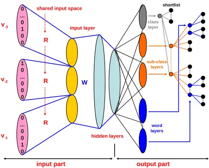
Neural network language models (Bengio et al., 2003) propose to represent words in a continuous space and to estimate the probability distribution as a smooth function of this representation. Figure 1 provides an overview of this approach. The context words are first projected in a continuous space using the shared matrixR. Denotingvthe1-of-V coding vector of wordv(all null except for thevth

compo-nent which is set to 1), its projection vector is the

vth line of R: RTv. The hidden layer h is then computed as a non-linear function of these vectors. Finally, the probability of all possible outcomes are computed using one or several softmax layer(s).

1

wji denotes a sequence of tokenswi. . . jwhenj ≥i, or

0 ... 0 1 0 0

1 0 ... 0 0 0

0 ... 0 0 1 0

v-3

v-2

v-1

R

R R

shared input space

input layer

hidden layers

shortlist

sub-class layers

word layers

class layer

input part output part

W

Figure 1:4-gram model with SOUL at the output layer.

This architecture can be divided in two parts, with the hidden layer in the middle: the input part (on the left hand side of the graph) which aims at represent-ing the context of the prediction; and the output part (on the right hand side) which computes the proba-bility of all possible successor words given the con-text. In the remaining of this section, we describe these two parts in more detail.

2.1 Input Layer Structure

The input part computes a continuous representation of the context in the form of a context vectorhto be processed through the hidden layer.

2.1.1 N-gram Input Layer

Using the standard n-gram assumption of equa-tion (2), the context is made up of the solen−1 pre-vious words. In a n-gram NNLM, these words are projected in the shared continuous space and their representations are then concatenated to form a sin-gle vectori, as illustrated in the left part of Figure 1:

i={RTv−(n−1);RTv−(n−2);. . .;RTv−1}, (3)

where v−k is thekth previous word. A non-linear

transformation is then applied to compute the first hidden layerhas follows:

h= sigm (Wi+b), (4)

withsigmthe sigmoid function. This kind of archi-tecture will be referred to as a feed-forward NNLM.

Conventional n-gram LMs are usually limited to small values ofn, and using n greater that 4 or 5

does not seem to be of much use. Indeed, previ-ous experiments using very large speech recognition systems indicated that the gain obtained by increas-ing the n-gram order from 4 to 5 is almost negli-gible, whereas the model size increases drastically. While using large context seems to be very imprac-tical with back-off LMs, the situation is quite dif-ferent for NNLMs due to their specific architecture. In fact, increasing the context length for a NNLM mainly implies to expend the projection layer with one supplementary projection vector, which can fur-thermore be computed very easily through a sim-ple look-up operation. The overall comsim-plexity of NNLMs thus only grows linearly withnin the worst case (Schwenk, 2007).

In order to better investigate the impact of each context position in the prediction, we introduce a slight modification of this architecture in a man-ner analog to the proposal of Collobert and Weston (2008). In this variation, the computation of the hid-den layer defined by equation (4) is replaced by:

h= sigm

max

k

WkRTv−k

+b

, (5)

whereWk is the sub-matrix ofW comprising the columns related to thekth_{history word, and themax}

is to be understood component-wise. The product

WkRT can then be considered as defining the pro-jection matrix for thekth_{position. After the}

projec-tion of all the context words, themax function se-lects, for each dimensionl, among then−1values ([WkRTv−k]l) the most active one, which we also

assume to be the most relevant for the prediction.

2.1.2 Recurrent Layer

Recurrent networks are based on a more complex architecture designed to recursively handle an arbi-trary number of context words. Recurrent NNLMs are described in (Mikolov et al., 2010; Mikolov et al., 2011b) and are experimentally shown to outper-form both standard back-off LMs and feed-forward NNLMs in terms of perplexity on a small task. The key aspect of this architecture is that the input layer for predicting theith_wordw

iin a text contains both

The hidden layer thus acts as a representation of the context history that iteratively accumulates an un-bounded number of previous words representations. Our reimplementation of recurrent NNLMs slightly differs from the feed-forward architecture mainly by its input part.We use the same deep archi-tecture to model the relation between the input word presentations and the input layer as in the recurrent model. However, we explicitly restrict the context to then−1previous words. Note that this architecture is just a convenient intermediate model that is used to efficiently train a recurrent model, as described in Section 3. In the recurrent model, the input layer is estimated as a recursive function of both the current input word and the past input layer.

i= sigm(Wi−1+RTv−1) (6)

As in the standard model,RTv−kassociates each context wordv−k to one feature vector (the corre-sponding row in R). This vector plays the role of a bias at subsequent input layers. The input part is thus structured in a series of layers, the relation tween the input layer and the first previous word be-ing at level1, the second previous word is at level2

and so on. In (Mikolov et al., 2010; Mikolov et al., 2011b), recurrent models make use of the entire con-text, from the current word position all the way back to the beginning of the document. This greatly in-creases the complexity of training, as each document must be considered as a whole and processed posi-tion per posiposi-tion. By comparison, our reimplemen-tation only considers a fixed context length, which can be increased at will, thus simulating a true recur-rent architecture; this enables us to take advantage of several techniques during training that speed up learning (see Section 3). Furthermore, as discussed below, our preliminary results show that restricting the context to the current sentence is sufficient to at-tain optimal performance2.

2.2 Structured Output Layer

A major difficulty with the neural network approach is the complexity of inference and training, which largely depends on the size of the output

vocabu-2_{The test sets used in MT experiments are made of various}

News extracts. Their content is thus not homogeneous and us-ing words from previous sentences doesn’t seem to be relevant.

lary ,i.e. of the number of words that have to be pre-dicted. To overcome this problem, Le et al. (2011a) have proposed the structured Output Layer (SOUL) architecture. Following (Mnih and Hinton, 2008), the SOUL model combines the neural network ap-proach with a class-based LM (Brown et al., 1992). Structuring the output layer and using word class in-formation makes the estimation of distribution over large output vocabulary computationally feasible.

In the SOUL LM, the output vocabulary is struc-tured in a clustering tree, where every word is asso-ciated to a unique path from the root node to a leaf node. Denotingwitheithword in a sentence, the

se-quencec1:D(wi) =c1, . . . , cD encodes the path for

word wi in this tree, withDthe tree depth, cd(wi)

the class or sub-class assigned towi, andcD(wi)the

leaf associated withwi, comprising just the word

it-self. The probability of wi given its history h can

then be computed as:

P(wi|h) =P(c1(wi)|h)

×

D

Y

d=2

P(cd(wi)|h, c1:d−1). (7)

There is a softmax function at each level of the tree and each word ends up forming its own class (a leaf). The SOUL architecture is represented in the right part of Figure 1. The first (class layer) estimates the class probability P(c1(wi)|h), while

sub-class layers estimate the sub-class probabili-ties P(cd(wi)|h, c1:d−1), d = 2. . .(D − 1). Fi-nally, theword layer estimates the word probabili-tiesP(cD(wi)|h, c1:D−1). As in (Schwenk, 2007), words in the short-list remain special, as each of them represents a (final) class on its own right.

3 Efficiency issues

Training a SOUL model can be achieved by maxi-mizing the log-likelihood of the parameters on some training corpus. Following (Bengio et al., 2003), this optimization is performed by Stochastic Back-Propagation (SBP). Recurrent models are usually trained using a variant of SBP called the Back-Propagation Through Time (BPTT) (Rumelhart et al., 1986; Mikolov et al., 2011a).

for instance, n-gram level resampling and bunch mode training with parallelization (see below); these methods can drastically reduce the overall training time, from weeks to days. Adapting these meth-ods to recurrent models are not straightforward. The same goes with the SOUL extension: its training scheme requires to first consider a restricted output vocabulary (the shortlist), that is then extended to in-clude the complete prediction vocabulary (Le et al., 2011b). This technique is too time consuming, in practice, to be used when training recurrent mod-els. By bounding the recurrence to a dozen or so previous words, we obtain a recurrent-like n-gram model that can benefit from a variety of speed-up techniques, as explained in the next sections.

Note that the bounded-memory approximation is only used for training: once training is complete, we derive a true recurrent network using the parameters trained on its approximation. This recurrent archi-tecture is then used for inference.

3.1 Reducing the training data

Our usual approach for training large scale models is based onn-gram levelresamplinga subset of the training data at each epoch. This is not directly com-patible with the recurrent model, which requires to iterate over the training data sentence-by-sentence in the same order as they occur in the document. How-ever, by restricting the context to sentences, data re-sampling can be carried out at the sentence level. This means that the input layer is reinitialized at the beginning of each sentence so as to “forget”, as it were, the memory of the previous sentences. A similar proposal is made in (Mikolov et al., 2011b), where the temporal dependencies are limited to the level of paragraph. Another useful trick, which is also adopted here, is to use different sampling rates for the various subparts of the data, thus boosting the use of in-domain versus out-of-domain data.

3.2 Bunch mode

Bunch modetraining processes sentences by batches of several examples, thus enabling matrix operation that are performed very efficiently by the existing BLAS library. After resampling, the training data is divided into several sentence flows which are pro-cessed simultaneously. While the number of exam-ples per batch can be as high as 128 without any

visible loss of performance forn-gram NNLM, we found, after some preliminary experiments, that the value of32seems to yield a good tradeoff between the computing time and the performance for recur-rent models. Using such batches, the training time can be speeded up by a factor of8at the price of a slight loss (less than2%) in perplexity.

3.3 SOUL training scheme

The SOUL training scheme integrates several steps aimed at dealing with the fact that the output vocab-ulary is split in two sub-parts: very frequent words are in the so-calledshort-list and are treated differ-ently from the less frequent ones. This setting can not be easily reproduced with recurrent models. By contrast, using the pseudo-recurrentn-gram NNLM, the SOUL training scheme can be adopted; the re-sulting parameter values are then plugged in into a truly recurrent architecture. In the light of the results reported below, we content ourselves with values of

nin the range8-10.

4 Experimental Results

We now turn to the experimental part, starting with a description of the experimental setup. We will then present an attempt to quantify the relative impor-tance of history words, followed by a head to head comparison of the various NNLM architectures dis-cussed in the previous sections.

4.1 Experimental setup

The tasks considered in our experiments are derived from the shared translation track of WMT 2011 (translation from English to French). We only pro-vide here a short overview of the task; all the neces-sary details regarding this evaluation campaign are available on the official Web site3 and our system is described in (Allauzen et al., 2011). Simply note that our parallel training data includes a large Web corpus, referred to as the GigaWord parallel cor-pus. After various preprocessing and filtering steps, the total amount of training data is approximately 12 million sentence pairs for the bilingual part, and about 2.5 billion of words for the monolingual part.

To built the target language models, the mono-lingual corpus was first split into several sub-parts

based on date and genre information. For each of these sub-corpora, a standard4-gram LM was then estimated with interpolated Kneser-Ney smoothing (Chen and Goodman, 1996). All models were cre-ated without any pruning nor cutoff. The baseline back-off n-gram LM was finally built as a linear combination of several these models, where the in-terpolation coefficients are chosen so as to minimize the perplexity of a development set.

All NNLMs are trained following the prescrip-tions of Le et al. (2011b), and they all share the same inner structure: the dimension of the projec-tion word space is 500; the size of two hidden lay-ers are respectively1000and500; the short-list con-tains2000words; and the non-linearity is introduced with the sigmoid function. For the recurrent model, the parameter that limits the back-propagation of er-rors through time is set to 9 (see (Mikolov et al., 2010) for details). This parameter can be considered to play a role that is similar to the history size in our pseudo-recurrentn-gram model: a value of9in the recurrent setting is equivalent to n = 10. All NNLMs are trained with the following resampling strategy:75%of in-domain data (monolingual News data 2008-2011) and25%of the other data. At each epoch, the parameters are updated using approxi-mately50 millions words for the last training step and about140millions words for the previous ones.

4.2 The usefulness of remote words

In this section, we analyze the influence of each con-text word with respect to their distance from the pre-dicted word and to their POS tag. The quantitative analysis relies on the variant of then-gram architec-ture based on (5) (see Section 2.1), which enables us to keep track of the most important context word for each prediction. Throughout this study, we will consider10-gram NNLMs.

Figure 2 represents the selection rate with respect to the word position and displays the percentage of coordinates in the input layer that are selected for each position. As expected, close words are the most important, with the previous word accounting for more than35% of the components. Remote words (at a distance between 7 and 9) have almost the same, weak, influence, with a selection rate close to

2.5%. This is consistent with the perplexity results ofn-gram NNLMs as a function of n, reported in

Tag Meaning Example

ABR abreviation etc FC FMI

ABK other abreviation ONG BCE CE ADJ adjective officielles alimentaire mondial ADV adverb contrairement assez alors

DET article; une les la

possessive pronoun ma ta INT interjection oui adieu tic-tac

KON conjunction que et comme

NAM proper name Javier Mercure Pauline

NOM noun surprise inflation crise

NUM numeral deux cent premier

PRO pronoun cette il je

PRP preposition; de en dans

preposition plus article au du aux des

PUN punctuation; : ,

-punctuation citation ”

SENT sentence tag ? . !

SYM symbol %

VER verb ont fasse parlent

<s> start of sentence

Table 1:List of grouped tags from TreeTagger.

Table 2: the difference between all orders from4 -gram to8-gram are significant, while the difference between8-gram and10-gram is negligible.

POS tags were computed using the TreeTag-ger (Schmid, 1994); sub-types of a main tag are pooled to reduce the total number of categories. For example, all the tags for verbs are merged into the same VER class. Adding the token<s>(sentence start), our tagset contains17tags (see Table 1).

The average selection rates for each tag are shown in Figure 3: for each category, we display (in bars) the average number of components that correspond to a word in that category when this word is in pre-vious position. Rare tags (INT, ABK , ABR and SENT) seem to provide a very useful information and have very high selection rates. Conversely, DET, PUN and PRP words occur relatively frequently and belong to the less selective group. The two most frequent tags (NOM and VER ) have a medium se-lection rate (approximately0.5).

4.3 Translation experiments

1 2 3 4 5 6 7 8 9 0.00

0.05 0.10 0.15 0.20 0.25 0.30 0.35

Figure 2:Average selection rate per word position for the

max-based NNLM, computed on newstest2009-2011. On xaxis, the numberkrepresents thekth_{previous word.}

0 5 10 15

0.0 0.2 0.4 0.6 0.8 1.0

PUN DET SYM PRP NUM KON ADV SENT PRO VER <s> ADJ NOM ABR NAM ABK INT

Figure 3: Average selection rate of max function of the first previous word in terms of word POS-tag information, computed on newstest2009-2011. The green line repre-sents the distribution of occurrences of each tag.

of each hypothesis is computed and thek-best list is accordingly reordered. The NNLM weights are op-timized as the other feature weights using Minimum Error Rate Training (MERT) (Och, 2003). For all our experiments, we used the valuek= 300.

To clarify the impact of the language model or-der in translation performance, we consior-dered three different ways to use NNLMs. In the first setting, the NNLM is usedaloneand all the scores provided by the MT system are ignored. In the second set-ting (replace), the NNLM score replaces the score of the standard back-off LM. Finally, the score of the NNLM can be added in the linear combination (add). In the last two settings, the weights used for

Model Perplexity BLEU

alone replace add

Baseline 90 29.4 31.3

-4-gram 92 29.8 31.1 31.5

6-gram 82 30.2 31.6 31.8

8-gram 78 30.6 31.6 31.8

10-gram 77 30.5 31.7 31.8

recurrent 81 30.4 31.6 31.8

Table 2: Results for the English to French task obtained with the baseline system and with various NNLMs. Per-plexity is computed on newstest2009-2011 while BLEU is on the test set (newstest2010).

n-best reranking are re-tuned with MERT.

Table 2 summarizes the BLEU scores obtained on thenewstest2010test set. BLEU improvements are observed with feed-forward NNLMs using a value of n = 8 with respect to the baseline (n = 4). Further increase from8 to10 only provides a very small BLEU improvement. These results strengthen the assumption made in Section 3.3: there seem to be very little information in remote words (above

n= 7-8). It is also interesting to see that the4-gram NNLM achieves a comparable perplexity to the con-ventional4-gram model, yet delivers a small BLEU increase in thealonecondition.

Surprisingly4_{, on this task, recurrent models seem}

to be comparable with 8-gram NNLMs. The rea-son may be the deep architecture of recurrent model that makes it hard to be trained in a large scale task. With the recurrent-like n-gram model described in Section 2.1.2, it is feasible to train a recurrent model on a large task. With10%of perplexity reduction as compared to a backoff model, its yields comparable performances as reported in (Mikolov et al., 2011a). To the best of our knowledge, it is the first recurrent NNLM trained on a such large dataset (2.5 billion words) in a reasonable time (about11days).

5 Related work

There have been many attempts to increase the context beyond a couple of history words (see eg. (Rosenfeld, 2000)), for example: by modeling

syn-4_{Pers. com. with T. Mikolov: on the ”small” WSJ data}

tactic information, that better reflects the “distance” between words (Chelba and Jelinek, 2000; Collins et al., 2005; Schwartz et al., 2011); with a unigram model of the whole history (Kuhn and Mori, 1990); by using trigger models (Lau et al., 1993); or by try-ing to model document topics (Seymore and Rosen-feld, 1997). One interesting proposal avoids then -gram assumption by estimating the probability of a sentence (Rosenfeld et al., 2001). This approach relies on a maximum entropy model which incor-porates arbitrary features. No significant improve-ments were however observed with this model, a fact that can be attributed to two main causes: first, the partition function can not be computed exactly as it involves a sum over all the possible sentences; sec-ond, it seems that data sparsity issues for this model are also adversely affecting the performance.

The recurrent network architecture for LMs was proposed in (Mikolov et al., 2010) and then ex-tended in (Mikolov et al., 2011b). The authors pro-pose a hierarchical architecture similar to the SOUL model, based however on a simple unigram clus-tering. For large scale tasks (≈ 400M training words), advanced training strategies were investi-gated in (Mikolov et al., 2011a). Instead of resam-pling, the data was divided into paragraphs, filtered and then sorted: the most in-domain data was thus placed at the end of each epoch. On the other hand, the hidden layer size was decreased by simulating a maximum entropy model using a hash function on

n-grams. This part represents direct connections be-tween input and output layers. By sharing the pre-diction task, the work of the hidden layer is made simpler, and can thus be handled with a smaller number of hidden units. This approach reintroduces into the model discrete features which are somehow one main weakness of conventional backoff LMs as compared to NNLMs. In fact, this strategy can be viewed as an effort to directly combine the two ap-proaches (backoff-model and neural network), in-stead of using a traditional way, through interpola-tion. Training simultaneously two different models is computationally very demanding for large vocab-ularies, even with help of hashing technique; in com-parison, our approach keeps the model architecture simple, making it possible to use the efficient tech-niques developed forn-gram NNLMs.

The use the max, rather than a sum, on the

hid-den layer of neural network is not new. Within the context of language modeling, it was first proposed in (Collobert et al., 2011) with the goal to model a variable number of input features. Our motivation for using this variant was different, and was mostly aimed at analyzing the influence of context words based on the selection rates of this function.

6 Conclusion

In this paper, we have investigated several types of NNLMs, along with conventional LMs, in or-der to assess the influence of long range dependen-cies within sentences in the language modeling task: from recurrent models that can recursively handle an arbitrary number of context words to n-gram NNLMs withnvarying between4and10. Our con-tribution is two-fold.

First, experimental results showed that the influ-ence of word further than9can be neglected for the statistical machine translation task5. Therefore, the

n-gram assumption withn≈10appears to be well-founded to handle most sentence internal dependen-cies. Another interesting conclusion of this study is that the main issue of the conventional n-gram model is not its conditional independence assump-tions, but the use of too small values forn.

Second, by restricting the context of recurrent net-works, the model can benefit of the advanced train-ing schemes and its traintrain-ing time can be divided by a factor8without loss on the performances. To the best of our knowledge, it is the first time that a re-current NNLM is trained on a such large dataset in a reasonable time. Finally, we compared these mod-els within a large scale MT task, with monolingual data that contains2.5 billion words. Experimental results showed that using long range dependencies (n= 10) with a SOUL language model significantly outperforms conventional LMs. In this setting, the use of a recurrent architecture does not yield any im-provements, both in terms of perplexity and BLEU.

Acknowledgments

This work was achieved as part of the Quaero Pro-gramme, funded by OSEO, the French State agency for innovation.

References

Alexandre Allauzen, Gilles Adda, H´el`ene Bonneau-Maynard, Josep M. Crego, Hai-Son Le, Aur´elien Max, Adrien Lardilleux, Thomas Lavergne, Artem Sokolov, Guillaume Wisniewski, and Franc¸ois Yvon. 2011. LIMSI @ WMT11. InProceedings of the Sixth Work-shop on Statistical Machine Translation, pages 309– 315, Edinburgh, Scotland.

Y Bengio, R Ducharme, P Vincent, and C Jauvin. 2003. A neural probabilistic language model. Journal of Ma-chine Learning Research, 3(6):1137–1155.

Thorsten Brants, Ashok C. Popat, Peng Xu, Franz J. Och, and Jeffrey Dean. 2007. Large language models in machine translation. InProceedings of the 2007 Joint Conference on Empirical Methods in Natural guage Processing and Computational Natural Lan-guage Learning (EMNLP-CoNLL), pages 858–867. Peter F. Brown, Peter V. deSouza, Robert L. Mercer,

Vin-cent J. Della Pietra, and Jenifer C. Lai. 1992. Class-based n-gram models of natural language. Comput. Linguist., 18(4):467–479.

Ciprian Chelba and Frederick Jelinek. 2000. Structured language modeling. Computer Speech and Language, 14(4):283–332.

Stanley F. Chen and Joshua Goodman. 1996. An empiri-cal study of smoothing techniques for language model-ing. InProc. ACL’96, pages 310–318, San Francisco. Michael Collins, Brian Roark, and Murat Saraclar.

2005. Discriminative syntactic language modeling for speech recognition. InProceedings of the 43rd Annual Meeting of the Association for Computational Linguis-tics (ACL’05), pages 507–514, Ann Arbor, Michigan, June. Association for Computational Linguistics. Ronan Collobert and Jason Weston. 2008. A

uni-fied architecture for natural language processing: deep neural networks with multitask learning. In Proc. of ICML’08, pages 160–167, New York, NY, USA. ACM.

Ronan Collobert, Jason Weston, L´eon Bottou, Michael Karlen, Koray Kavukcuoglu, and Pavel Kuksa. 2011. Natural language processing (almost) from scratch. Journal of Machine Learning Research, 12:2493– 2537.

Ahmad Emami, Imed Zitouni, and Lidia Mangu. 2008. Rich morphology based n-gram language models for arabic. InINTERSPEECH, pages 829–832.

R. Kuhn and R. De Mori. 1990. A cache-based natural language model for speech recognition. IEEE Trans-actions on Pattern Analysis and Machine Intelligence, 12(6):570–583, june.

Hong-Kwang Kuo, Lidia Mangu, Ahmad Emami, and Imed Zitouni. 2010. Morphological and syntactic fea-tures for arabic speech recognition. InProc. ICASSP 2010.

Raymond Lau, Ronald Rosenfeld, and Salim Roukos. 1993. Adaptive language modeling using the maxi-mum entropy principle. InProc HLT’93, pages 108– 113, Princeton, New Jersey.

Hai-Son Le, Ilya Oparin, Alexandre Allauzen, Jean-Luc Gauvain, and Franc¸ois Yvon. 2011a. Structured out-put layer neural network language model. In Proceed-ings of ICASSP’11, pages 5524–5527.

Hai-Son Le, Ilya Oparin, Abdel. Messaoudi, Alexan-dre Allauzen, Jean-Luc Gauvain, and Franc¸ois Yvon. 2011b. Large vocabulary SOUL neural network lan-guage models. InProceedings of InterSpeech 2011. Xunying Liu, Mark J. F. Gales, and Philip C. Woodland.

2011. Improving lvcsr system combination using neu-ral network language model cross adaptation. In IN-TERSPEECH, pages 2857–2860.

Tom´aˇs Mikolov, Martin Karafi´at, Luk´aˇs Burget, Jan ˇ

Cernock´y, and Sanjeev Khudanpur. 2010. Recurrent neural network based language model. InProceedings of the 11th Annual Conference of the International Speech Communication Association (INTERSPEECH 2010), volume 2010, pages 1045–1048. International Speech Communication Association.

Tom´aˇs Mikolov, Anoop Deoras, Daniel Povey, Luk´aˇs Burget, and Jan ˇCernock´y. 2011a. Strategies for train-ing large scale neural network language models. In Proceedings of ASRU 2011, pages 196–201. IEEE Sig-nal Processing Society.

Tom´aˇs Mikolov, Stefan Kombrink, Lukas Burget, Jan Cernock´y, and Sanjeev Khudanpur. 2011b. Exten-sions of recurrent neural network language model. In Proc. of ICASSP’11, pages 5528–5531.

Andriy Mnih and Geoffrey E Hinton. 2008. A scalable hierarchical distributed language model. In D. Koller, D. Schuurmans, Y. Bengio, and L. Bottou, editors, Ad-vances in Neural Information Processing Systems 21, volume 21, pages 1081–1088.

Franz Josef Och. 2003. Minimum error rate training in statistical machine translation. In Proceedings of the 41st Annual Meeting on Association for Compu-tational Linguistics - Volume 1, ACL ’03, pages 160– 167, Stroudsburg, PA, USA. Association for Compu-tational Linguistics.

Ronald Rosenfeld, Stanley F. Chen, and Xiaojin Zhu. 2001. Whole-sentence exponential language models: A vehicle for linguistic-statistical integration. Com-puters, Speech and Language, 15:2001.

R. Rosenfeld. 2000. Two decades of statistical language modeling: Where do we go from here ? Proceedings of the IEEE, 88(8).

internal representations by error propagation, pages 318–362. MIT Press, Cambridge, MA, USA.

Helmut Schmid. 1994. Probabilistic part-of-speech tag-ging using decision trees. InProceedings of Interna-tional Conference on New Methods in Language Pro-cessing.

Lane Schwartz, Chris Callison-Burch, William Schuler, and Stephen Wu. 2011. Incremental syntactic lan-guage models for phrase-based translation. In Pro-ceedings of the 49th Annual Meeting of the Associa-tion for ComputaAssocia-tional Linguistics: Human Language Technologies, pages 620–631, Portland, Oregon, USA, June. Association for Computational Linguistics. Holger Schwenk and Jean-Luc Gauvain. 2002.

Connec-tionist language modeling for large vocabulary contin-uous speech recognition. InProc. ICASSP, pages 765– 768, Orlando, FL.

H. Schwenk and P. Koehn. 2008. Large and diverse lan-guage models for statistical machine translation. In International Joint Conference on Natural Language Processing, pages 661–666, Janv 2008.

Holger Schwenk. 2007. Continuous space language models. Comput. Speech Lang., 21(3):492–518. Kristie Seymore and Ronald Rosenfeld. 1997. Using

story topics for language model adaptation. InProc. of Eurospeech ’97, pages 1987–1990, Rhodes, Greece. Yeh W. Teh. 2006. A hierarchical Bayesian language