Optimizing End-to-End System Performance for Millimeter and Submillimeter Spectroscopy of Protostars: Wideband Heterodyne Receivers and Sideband-Deconvolution Techniques for Rapid Molecular-Line Surveys

(1)

Submillimeter Spectroscopy of Protostars:

Wideband Heterodyne Receivers and Sideband-Deconvolution

Techniques for Rapid Molecular-Line Surveys

Thesis by Matthew C. Sumner

In Partial Fulfillment of the Requirements for the Degree of

Doctor of Philosophy

California Institute of Technology Pasadena, California

2011

(2)

c

2011

(3)

(4)

(5)

Acknowledgements

I would like to offer my deep gratitude to the following people for making this work possible:

Jonas Zmuidzinas for his faith in me, for standing by me during the challenging times, for his generous support of his students, and for seeing every setback as an exciting opportunity to understand the problem better.

My wife, Heather, for her constant love and support, for all the fun times we have had during this process, and for the many, many sacrifices she has made to allow me to complete my degree.

My children, Claire and David, for bringing joy and sunshine into every day, for their patience on all the nights and weekends that I spent in the office finishing this work, and for helping me to keep perspective on the things that really matter in life.

My parents, Jim and Molly, for always believing in me, for starting me on the path that has led to this point, and for lending a sympathetic ear whenever I needed support.

Sue, Roger, Laura, and Greg for never doubting that I would finish, for welcoming me into their family, and for supporting me in the final stretch. I would particularly like to thank Sue for flying down on a moment’s notice and for staying weeks at a time to help us out while I finished my thesis.

(6)

Tom Phillips for his commitment to mentoring students, particularly his generosity with telescope time in support of students’ work, and for always being willing to pull up a chair atHale Pohakufor a friendly conversation over dinner.

Geoff Blake for his enthusiasm, for his focus on helping me to graduate quickly, and for his help at the summit when we were taking the data used in this work.

Ernie from the “Ernie’s al Fresco” lunch truck, for making sure I had a warm lunch and a kind word every day.

Joseph V. for jumping in and running the final lap at my side, offering moral support and practical advice every step of the way.

Alice S. for her professional guidance and for a friendship that endured throughout my time at Caltech.

(7)

Abstract

This thesis describes the construction, integration, and use of a new 230-GHz ultra-wideband heterodyne receiver, as well as the development and testing of a new sideband-deconvolution algorithm, both designed to enable rapid, sensitive molecular-line surveys.

The 230-GHz receiver, known as Z-Rex, is the first of a new generation of wideband receivers to be installed at the Caltech Submillimeter Observatory (CSO). Intended as a proof-of-concept device, it boasts an ultra-wide IF output range of∼6 - 18 GHz, offering as much as a twelvefold increase in the spectral coverage that can be achieved with a single LO setting. A similarly wideband IF system has been designed to couple this receiver to an array of WASP2 spectrometers, allowing the full bandwidth of the receiver to be observed at low resolution, ideal for extra-galactic redshift surveys. A separate IF system feeds a high-resolution 4-GHz AOS array frequently used for performing unbiased line surveys of galactic objects, particularly star-forming regions. The design and construction of the wideband IF system are presented, as is the work done to integrate the receiver and the high-resolution spectrometers into a working system. The receiver is currently installed at the CSO where it is available for astronomers’ use.

(8)

The receiver and high-resolution spectrometer system were brought into a fully opera-tional state late in 2007, when they were used to perform unbiased molecular-line surveys of several galactic sources, including the Orion KL hot core and a position in the L1157 outflow. In order to analyze these data, a new data pipeline was needed to deconvolve the double-sideband signals from the receiver and to model the molecular spectra. A highly automated sideband-deconvolution system has been created, and spectral-analysis tools are currently being developed.

The sideband deconvolution relies on chi-square minimization to determine the op-timal single-sideband spectrum in the presence of unknown sideband-gain imbalances and spectral baselines. Analytic results are presented for several different methods of ap-proaching the problem, including direct optimization, nonlinear root finding, and a hybrid approach that utilizes a two-stage process to separate out the relatively weak nonlineari-ties so that the majority of the parameters can be found with a fast linear solver. Analytic derivations of the Jacobian matrices for all three cases are presented, along with a new

Mathematicautility that enables the calculation of arbitrary gradients.

The direct-optimization method has been incorporated into software, along with a spectral simulation engine that allows different deconvolution scenarios to be tested. The software has been validated through the deconvolution of simulated data sets, and initial results from L1157 and Orion are presented.

(9)

Chapter 1

Introduction

1.1

Star Formation

Throughout most of the interstellar medium, atomic species dominate. The density is so low that interactions between atoms are rare, and any molecules that do form are de-stroyed almost immediately by stellar radiation. Within this harsh environment, however, there are oases in the form of molecular clouds. These clouds consist of dense collections of dust and gas in which the outer layers of dust grains protect the interiors of the clouds from stellar radiation. The higher density provides more opportunities for atoms to inter-act and form molecules while the gentler environment allows those molecules to survive.

(14)

Figure 1.1: Overview of low-mass star formation.

allowing matter to accrete onto the central source. In this model, excess angular momen-tum is carried off by magnetically driven jets emanating from both poles of the protostar.

Most of the gas inside a molecular cloud is relatively cold, with temperatures on the order of T ∼ 10 - 20 K [Gueth et al., 1997, Shu et al., 1993]. At this stage of stellar de-velopment, the protostar is not massive enough to support internal burning. However, the gravitational potential energy given up by material falling into the central protostar releases a significant amount of energy, which is eventually converted into heat in the sur-rounding gas.1 This increased thermal energy allows the relatively simple molecules of the molecular cloud to interact with one another, driving a surprisingly rich chemistry.

As the protostar evolves into a so-called Class I object, the amount of matter falling onto the central source decreases. The angular extent of the bipolar jets expands, gradu-ally clearing the remains of the dense core. The protostar continues to evolve into a Class II

1_{In high-mass protostars, some of the richest chemistry occurs in the hot core, the warm region near the}

(15)

Figure 1.2: Artist’s conception of a heavily enshrouded protostar. (Image courtesy of NASA/JPL-Caltech/R. Hurt, SSC.)

object, characterized by a fully exposed central source surrounded by a dusty, protoplane-tary disk, and finally a Class III object, in which disk-clearing has condensed much of the diffuse material of the disk into planets.

1.2

Studying Molecular Clouds

Molecular clouds exist because dust grains shield the interiors from intense optical and ultraviolet stellar radiation; however, this also makes them difficult to study at many of the traditional wavelengths. In particular, the same dust grains that keep light from entering also prevent it from escaping, making it impossible to study the interiors of molecular clouds with optical observations.

(16)

As an example, consider the images of the Carina Nebula in Figure 1.3. The top image shows a dust pillar in the visible spectrum while the bottom shows the same image in infrared. Because of their longer wavelengths, the infrared photons are not scattered as heavily by the dust. They escape from the depths of the molecular cloud, making the dust virtually invisible and clearly revealing an embedded protostar (and its associated outflows) at the tip of the dust column.

The situation improves further when even longer wavelengths are used, as shown in Figure 1.4, comparing visible and submillimeter images of the Antennae Galaxies.2 The interactions between these colliding galaxies has stirred the dust and gas, triggering star formation. This fact is not obvious in the visible image, but appears clearly in the submil-limeter, where the bright red regions show dense dust that has been warmed by obscured star formation.

Submillimeter observations benefit not only from an improved ability to penetrate through dust, but also because they are directly sensitive to emissions from the gas and dust in the star-forming regions. At the temperatures typical of these objects, thermal emission from the dust peaks at frequencies of a few to tens of THz, generating a signif-icant amount of flux at the upper end of the submillimeter range [Kraus, 1986, esp. Fig 3.16]. Because the peak of the emission occurs to the short side of the submillimeter range, submillimeter imaging arrays (such as SHARC II, which generated the data shown in Fig-ure 1.4) are ideal for searching for distant star-forming regions in which the spectrum has been redshifted.

Not surprisingly, molecular clouds also generate a significant amount of flux in molec-ular emission lines. In particmolec-ular, the temperatures are just right to excite the low-lying ro-tational (and sometimes vibrational) quantum levels of small molecules, and the resulting rovibrational emission spectral lines lie squarely in the submillimeter range. For instance, CO, one of the most common interstellar molecules, has strong emission lines spaced at 115 GHz, and the lines at 230 GHz and 345 GHz are particularly useful tracers of molecular gas.

2_{Submillimeter and millimeter wavelengths fall between microwave and far-infrared. The submillimeter}

image shown here was taken by the SHARC II camera, operating at 350µm (≈850 GHz). The term

(17)

(18)

(19)

1.3

Interplay between Physics and Chemistry

As Groesbeck et al. [1994] demonstrated, the integrated flux in the molecular lines may represent a significant fraction of, or even the majority of, the energy emitted from star-forming regions in the submillimeter range. This means that instruments sensitive to that emission make great tools for studying such regions, but it also implies something impor-tant about the physics of star formation. As stated earlier, the gas and dust falling onto the central core of a protostar give up a considerable amount of gravitational potential en-ergy that eventually is converted into heat. In order to continue to collapse, the gas in and around the protostar must have some way of dissipating this heat. While thermal emission from dust plays a key role, cooling via molecular-line emission is also critical to the pro-cess. Thus, in order to fully describe star formation, one must understand the line emission from the region, which in turn, requires a knowledge of the molecular constituents.

Understanding the astrochemistry of star formation is also important for establishing the physical state of material surrounding a protostar. Throughout much of a molecular cloud, a significant portion of the molecular gas is believed to be frozen into ices that coat the surfaces of dust grains [Boogert, 1999]. The warmth generated by stellar formation causes these ices to sublimate, increasing the density of the gas-phase material near the protostar. In order to calculate the details of this density profile, it is necessary to under-stand the constituents of the molecular ices.

Similarly, the physics of star formation has a strong effect on the associated astrochem-istry. Without the thermal energy generated by the infalling matter, most of the molecules would remain frozen on dust grains, constraining the types of reactions they could un-dergo. The gas-phase density has direct consequences for the likelihood of collisions be-tween molecules while the physical size of a star-forming region sets a distance scale over which one molecule must encounter another if it is to react before drifting out into the colder reaches of the molecular cloud. In addition, the powerful outflows from a protostar create their own chemistry, both within the ejected material and at the shock front that results from the outflow plowing into the quiescent envelope.

(20)

Figure 1.5: 795 - 903 GHz survey of Orion by Comito et al. [2005]. The atmospheric trans-mission typical of the observing conditions for the survey (shown in gray in the back-ground of the plot) testifies to the difficulty of this work.

1.4

Submillimeter Line Surveys

One particularly powerful way to study star-forming regions is through the use of unbi-ased submillimeter line surveys, in which molecular lines are observed over a broad range of frequencies. Figure 1.5 shows a survey of the Orion molecular cloud from 795 - 903 GHz [Comito et al., 2005], showing a wealth of lines, even at these relatively high frequencies.

In contrast to targeted line studies, which seek to confirm or refute the existence of a particular molecular line, an unbiased survey seeks to inventory all of the lines within the observing window. This information can be used to build up a “chemical catalog” for the star-forming region, placing important constraints on models and helping to distinguish between competing descriptions of astrochemical networks.

(21)

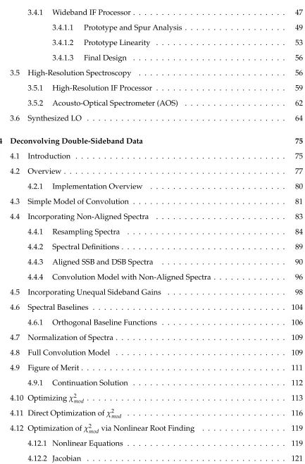
Figure 1.6: Decomposition of spectral line in OMC-1 survey. From Blake et al. [1987, Fig. 2].

By directly probing the molecular gas, a line survey provides a wealth of information about chemical and physical conditions within the star-forming region. Line frequencies can be used to identify molecular species while the line profiles give important information about source dynamics. Amplitudes of lines can be used to estimate physical conditions in the source, such as temperature, pressure, and density, particularly when many molecules, each with multiple lines, are observed.

As an example, consider the peak shown in Figure 1.6, taken from a survey of the Orion molecular cloud (OMC-1). As described in Blake et al. [1987], the observed spectral line, shown at the top, can be decomposed into contributions from several physically distinct regions based on the line profile, as shown in the remaining three traces in the figure. The bottom line (labeled “Hot Core”) corresponds to gas warmed by the central source while the narrow “Ridge” line represents quiescent gas unaffected by the protostar’s creation in its midst. The very broad tails of the “Plateau” line tie it to the powerful outflows driven by the protostar. Such analysis not only helps to identify the dynamics of the source, but also allows the chemistry of each region to be analyzed separately, even when the lines are blended together.

(22)

often spans multiple observing runs, sometimes extending across several years. Not only does this represent a significant allocation of resources, but changes in the telescope or receiver configuration can make it difficult to stitch the different data sets together into a single spectrum.

One of the first major surveys of a star-forming region was completed by Blake and Sutton, who studied the Orion molecular cloud from 215 - 263 GHz [Blake et al., 1986, Sutton et al., 1985]. That survey consisted of more than 100 independent observations over 28 nights spread across two adjacent winters. The 795 - 903 GHz survey of the same source, shown in Figure 1.5, required a total of 300 independent observations spread over an approximately five-year period [Comito et al., 2005]. Just the upper half of the spectrum (from 845 - 903 GHz) required 30 nights of observing time, largely due to the challenge of observing at near-THz frequencies from a ground-based telescope.

In Schilke et al. [1997], the authors point out that completing the observations and assembling them into a coherent spectrum is just the beginning and that the truly time-consuming part is the spectral analysis and interpretation. Thus, while line surveys pro-vide a wealth of data, the information is hard-won.

1.5

Instrumentation for Line Surveys

Submillimeter line surveys of star-forming regions are nearly always performed using het-erodyne spectroscopy, with an instrumental configuration similar to that shown in Figure 1.7. Photons collected by the telescope are focused onto a mixer, where they are combined with a reference signal generated by a local oscillator (LO). The mixer consists of a device with a nonlinear relationship between current and voltage (a nonlinear I-V curve), which results in the multiplication of the two input signals. The output consists of two signals, one at a frequency equal to the sum of the two input frequencies, and one equal to the difference between them. Only the difference signal is needed for this application, so the sum frequency is removed using a filter. From there, the signal is amplified and passed to a spectrometer, which generates the desired spectrum.

(23)

Figure 1.7: Basic instrumentation needed for heterodyne spectroscopy.

commercial, off-the-shelf amplifiers, filters, and connectors are readily available, making it vastly easier and cheaper to work with the signal. This configuration also provides modularity that allows the front-end mixers to be designed separately from the back-end spectrometers. For instance, at the CSO, there are multiple receivers, covering frequencies from 180 GHz up to 900 GHz. They are configured to convert the sky radiation to a com-mon frequency on the output, allowing a single set of spectrometers to be used for all of them.

Scientifically, heterodyne spectroscopy is desirable because it offers extremely high fre-quency resolution, which is critical for studying molecular-line spectra of star-forming regions. A sample spectrum from the Orion survey is shown in Figure 1.8, demonstrating the fine details that must be preserved. The narrower peaks are only a few MHz wide and the CH3OH and HNCO lines near the center of the spectrum have frequencies of 241.767

GHz and 241.774 GHz, corresponding to a 7-MHz separation.

(24)

Figure 1.8: A sample molecular-line spectrum from 241.5 - 242 GHz [Sutton et al., 1985].

1.6

Sideband Ambiguity

Heterodyne spectroscopy is well suited to the study of submillimeter molecular lines, but there is one difficulty that it introduces. The goal of a line survey is to produce frequency-calibrated spectra like the one shown in Figure 1.8, in which each channel of the spectrum can be concretely identified with a single frequency. However, at most telescopes (includ-ing the CSO), each channel in a heterodyne spectrum actually corresponds totwo frequen-cies; it can only be reduced to the form shown above with a significant amount of data processing.

More detail is given in Chapter 4, but the basic problem can be demonstrated by re-considering the simple system shown in Figure 1.7. In Figure 1.9, we show the same system with the addition of frequency labels. Start by considering the general variables shown in the boxes attached to each of the black arrows. The telescope collects pho-tons with frequency fRF while the LO generates a signal at frequency fLO. In the mixer, these are multiplied to produce the sum and difference frequencies, fSU M= fLO+ fRFand

fDIFF = |fLO− fRF|, respectively. The filter removes the sum frequency, leaving only the difference frequency, fDIFF, at the input to the spectrometer.

(25)

Figure 1.9: Frequency conversions in a simple double-sideband receiver, showing the ori-gin of the sideband ambiguity.

result can be achieved by considering a 245-GHz input to the telescope. The difference frequency will still be 5 GHz, so the input to the spectrometer will be identical in both cases.

Given the knowledge that the spectrometer observed a 5-GHz peak while using a 240-GHz LO setting, we can only say that the input must have contained some combination of 235-GHz and 245-GHz signals. This uncertainty is known as the sideband ambiguity, and it is inherent to the single-mixer receiver design outlined above. It is possible to remove this ambiguity during the data-analysis stage via a process known as sideband deconvo-lution, which will be covered extensively in Chapter 4.

(26)

1.7

Goals of This Work

This thesis describes an effort to enable rapid, unbiased molecular-line surveys at sub-millimeter frequencies with the goal of allowing such surveys to be performed more fre-quently and to achieve higher sensitivities.

Because of the difficulties of performing such work, only a few sources have been sur-veyed to date, and significant pieces of our understanding of star formation have been extrapolated from these objects. Making it easier to complete a line survey would allow astronomers to study many more objects, eventually building up a statistical sample of sources that could help to elucidate the different mechanisms at play.

One particularly intriguing line of inquiry is the search for “chemical clocks,” molecu-lar tracers that would help to identify the ages of different sources. Currently, estimating the age of a protostar requires subtle inference from a variety of observations; finding a molecular tracer that could serve as a proxy for the protostar’s age would greatly sim-plify the process. While efforts have been made to find such tracers through targeted line observations, a broad sample of unbiased line surveys would make the task significantly easier.

Improved survey methods would also offer the ability to take more sensitive line sur-veys. As models of astrochemistry improve, more sensitive observations are needed to distinguish between them, usually to look for peaks from complex molecules that are pre-dicted by the models but are lost in the noise of prior surveys. Likewise, unambiguously identifying prebiotic molecules requires sufficient sensitivity to dig multiple molecular lines out of the noise.

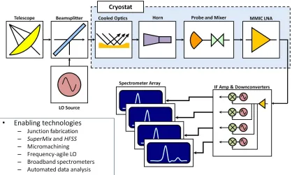
Accomplishing these goals has required the development of new hardware and soft-ware. Improvements in computer models, chip fabrication, and micromachining capabil-ities have allowed our group to design a new generation of ultra-wideband heterodyne receivers. In a single observation, these receivers can produce several times as much data as previous receivers, allowing a line survey to be completed with many fewer indepen-dent observations.

(27)

individual observations by hand, using a computer to perform the sideband deconvolution and assemble the observations into a single spectrum, and then manually fitting each peak in the resulting spectrum.

We have streamlined the analysis process by developing deconvolution algorithms that dramatically reduce the amount of manual processing required for each observation while still preserving the high sensitivity needed to search for complex and/or prebiotic mod-ules. Susanna Widicus Weaver’s group at Emory University is addressing the final part of the problem by developing spectral-fitting software that not only fits all of the lines of a given molecule simultaneously, but also fits several molecules at once.

(28)

(29)

Chapter 2

Submillimeter Observations

Before describing the construction of heterodyne receivers, we include a quick discussion of how submillimeter spectra are actually measured. Most of the signal for a submillimeter heterodyne receiver consists of thermal noise. The primary source of background is ther-mal emission by molecules in the atmosphere (especially water). The astronomical source adds a small bit of power on top of this, and the challenge is to separate out that small signal against the much larger background. This is the primary reason submillimeter tele-scopes are typically located at high elevations. The amount of water in the atmosphere falls off rapidly as a function of elevation; by observing at higher locations, astronomers can reduce the total amount of water between the telescope and the astronomical source.

As a concrete example, consider observations made under typical conditions at the Caltech Submillimeter Observatory (CSO), located at an elevation of 13,350 feet, near the summit of Mauna Kea (Figure 2.1). The 225-GHz opacity at zenith is usually τ225 ∼ 0.1,

and observations are performed at moderate zenith angles, corresponding to an airmass of A∼ 1.5. The signal from an astronomical source at 225 GHz would therefore be atten-uated by a factor ofe−Aτ225 _≈ _{0.86. In addition to attenuating the signal, the atmosphere}

introduces noise equal toT_sky= (1−e−Aτ225₎_T

atm, whereTatmis the temperature of the at-mosphere, usually assumed to be roughly the same as the ambient temperature at ground level (Tatm ∼ 300 K.1 Thus, the atmosphere contributes a signal of ∼ 28 K of noise per

1_{This assumption is justified by the fact that atmospheric pressure follows an exponential drop-off as a}

(30)

(31)

sideband, or∼ 56 K total. This is quite large in comparison to the desired spectral lines, which typically have peaks of amplitude∼0.1 - 10 K, or the continuum radiation, which is usually a few Kelvins.

To detect these small signals against the larger background, the CSO uses chopping subtraction, in which the source is observed for several seconds, and then an off-source position is observed for the same amount of time. As long as the length of each observation is much smaller than the timescale on which the atmospheric opacity changes, the average sky noise can be subtracted off, and the difference between these two signals represents the desired spectrum.

While the emission from the sky is viewed as “noise,” and the source’s emission is viewed as “signal,” it is important to emphasize that both arise from thermal emission. Therefore, the difference between them is also a random quantity, and it is this randomness that determines the sensitivity of the observation. The RMS noise in the signal after the subtraction is described by the Dicke radiometer equation,

T_RMSSSB = _p2Tsys

∆f ton

, (2.1)

where ∆f represents the bandwidth of the observation (e.g., one spectral channel), Tsys represents the system noise temperature andtonrepresents the on-source integration time.2

2_{Actually, a few intermediate steps are needed to arrive at the results shown in Equation 2.1. The Dicke}

radiometer equation describes the best possible performance that could be achieved by a device that takes an input signal, limits its frequency range to ∆f (e.g., with a bandpass filter), measures the power with a square-law detector, and then averages that result over a timeton. If we convert the measured power into an equivalent temperature, the uncertainty in that value must be at least

σT= Tsys

p

∆f ton

(2.2)

[Rohlfs and Wilson, 2003]. A spectrometer channel receiving input from a DSB receiver sums the input from two sidebands, increasing the noise by a factor of√2. The desired signal represents the difference of two such measurements taken in on-source and off-source positions: Tsource =Ton−To f f. If we observe the “on” and “off” positions for equal time, each has an uncertainty equal to

σTon =σTo f f =

√

2Tsys

p

∆f ton

. (2.3)

Standard propagation-of-error techniques can be used to determine the uncertainty inTsource:

σTsource=

√

2σTon=

2Tsys

p

∆f ton

. (2.4)

(32)

2.1

Calibration at the CSO

Submillimeter spectra are calibrated in a fashion that allows the underlying source spec-trum to be determined, independent of atmospheric conditions. Conceptually, the cali-brated data can be viewed as the spectrum that would be seen by an ideal telescope placed above Earth’s atmosphere, except with an additional amount of noise.

The CSO uses the chopper-wheel calibration method, as discussed in Kutner and Ulich [1981], Ulich and Haas [1976], and Peng [2002, Appendix A]. Before taking a spectrum, a calibration scan is calculated by comparing the spectrum of a hot load to that of a cold load. The loads are presumed to be perfect blackbodies over the frequencies of interest, so they can be characterized by a single, frequency-independent temperature. The hot load consists of an ambient-temperature absorber inserted into the beam of the receiver between the receiver and secondary mirror while the cold load is simply an empty patch of sky close to the astronomical source. As described in the following discussion, these observations can be used to determine two unknowns: the system’s gain and the end-to-end noise level.

A perfect receiver would be equally sensitive to signals in the upper and lower side-bands. In reality, the receiver often has slightly different sensitivity at the two frequencies. We can model this difference by lettingG(f)represent the receiver’s gain as a function of frequency. The gain represents the conversion factor between the spectrometer output and an astrophysically meaningful brightness temperature,T_A∗.3

Consider the output of a single channel of the spectrometer, represented asV.4 When presented with the hot load at temperatureT_hot, the spectrometer’s response is

Vhot= GLSB

Thot+TRxLSB

+GUSB

Thot+TRxUSB

, (2.5)

3_{There are a variety of temperature scales used for submillimeter spectra.} _T∗

Ais a common scale, as it can be derived directly from the chopper-wheel calibration. Values ofT∗_Ahave been corrected for atmospheric losses, ohmic losses in the telescope, and rear (warm) spillover. They havenotbeen corrected for forward (cold) spillover or the coupling between the telescope’s beam pattern and the source. See Kutner and Ulich [1981] for additional details.

4_{The quantity}_V_{is traditionally considered as a voltage, but it could represent other forms of spectrometer}

(33)

where the gains

GLSB = G(fLSB) and

GUSB = G(fUSB)

represent the LSB and USB gains at frequencies

fLSB = fLO− fIFand

fUSB = fLO+ fIF.

The two termsGLSB ThotandGUSB Thotsimply represent the receiver’s downconversion of power in the lower and upper sidebands. The receiver noise temperature TRx represents the noise added by the receiver during the downconversion. Conceptually, the receiver can be viewed as a perfect receiver, adding no noise to the signal, plus a noise source at the input with temperatureTRx. The receiver noise temperature is not necessarily frequency-independent, so the equation includes different values for the upper and lower sidebands. The response when looking at a blank patch of sky is a bit more complicated. While the majority of the signal comes from the primary beam, there are also contributions from spillover, scattering, and diffraction. Some of these effects produce rays that terminate on the sky, but not on the intended observation point while others result in rays that terminate on warm objects, such as the ground or the telescope structure. To model these effects, we introduce the warm and cold efficiencies, ηwarm and ηcold. These quantities are defined such that the fraction of the beam that terminates on a warm load is (1−ηwarm)while the fraction reaching the sky is ηwarm. Of that, η_cold forms the primary beam while the

remaining(1−ηcold)ends up on other sections of the sky.

The sky signal includes the following contributions for each side band:

(1−ηwarm)Thot

| {z }

Scattered into warm load

+ ηwarm(1−ηcold)Tsky

| {z }

On sky but outside main beam

+ ηwarmηcoldTsky

| {z }

Main beam

+ TRx

|{z}

Receiver noise

.

(34)

Vsky =GLSB h

(1−ηwarm)Thot+ηwarm(1−ηcold)TskyLSB+ηwarmηcoldTskyLSB+TRxLSB i

+GUSBh(1−ηwarm)Thot+ηwarm(1−η_cold)T_skyUSB+ηwarmη_coldT_skyUSB+T_RxUSB

i

,

which can be rearranged to

V_sky =GLSBh(1−ηwarm)Thot+ηwarmTskyLSB+TRxLSB i

+GUSBh(1−ηwarm)Thot+ηwarmTskyUSB+TRxUSB

i

. (2.6)

The sky temperature, T_sky, represents the effective temperature of the sky at the input to the receiver. The sky introduces noise into the spectrum with a brightness temperature of

Tsky =

1−e−Aτ_T

atm+

e−Aτ_T

space,

where τ represents the optical depth at the given frequency. A small amount of

radi-ation can be traced to even an “empty” patch of sky, primarily due to the cosmic mi-crowave background. However, the contribution is sufficiently small that it can be ne-glected: Tspace ≈ 0. As discussed in Footnote 1, the atmospheric temperature is usually approximated as the ambient temperature on the ground, Tatm ≈ Thot [Peng, 2002]. The sky opacity can be significantly different for the USB and LSB, particularly if one sideband is near a strong absorption line from atmospheric molecules. Therefore, whileThotmay be treated as a constant in the equation forVhot,Tskymust be defined separately for each side-band. The sky attenuation in the lower sideband is given bye−AτLSB_{for the lower sideband} ande−AτUSB _{for the upper sideband. We can define ¯}_τ_and_δτ_{such that}_τLSB ₌ _τ_¯₋_δτ_and

τUSB = τ¯ +δτ. Then the attenuation factors becomee−A(τ¯−δτ) ande−A(τ¯+δτ) for the LSB

and USB, respectively. To further simplify the notation, we let ¯ηsky = e−Aτ¯,η_skyLSB =+Aδτ,

andηUSB_sky =−Aδτ, giving

T_skyLSB =1−η¯_skyη_skyLSB

T_hotand

T_skyUSB = 1−η¯skyη_skyUSB

Thot.

(35)

These values can be inserted into Equation 2.6 to give

Vsky =GLSB h

(1−ηwarm)Thot+ηwarm

1−η¯skyη_skyLSB

Thot+TRxLSB i

+GUSBh(1−ηwarm)Thot+ηwarm

1−η¯_skyηUSB_sky

T_hot+T_RxUSBi,

which can be simplified to

V_sky =GLSBh1−ηwarmη¯_skyη_skyLSB

T_hot+T_RxLSBi

+GUSBh1−ηwarmη¯skyη_skyUSB

Thot+TRxUSB i

. (2.8)

When the telescope is pointed at an astronomical source, the signal contains all the components present inVsky, with an additional signal that can be attributed to the source:

Vsrc=Vsky+ηsrcηwarmη_coldη¯_sky

GLSBη_skyLSBT_srcLSB+GUSBη_skyUSBT_srcUSB

. (2.9)

The source-coupling efficiency,ηsrc, represents the convolution of the source structure with the telescope’s main-beam pattern and accounts for effects such as beam dilution whileTsrc is the effective temperature of the source.5

The spectra created by the CSO are calibrated to theT_A∗ scale using the following equa-tion [Peng, 2002, Equaequa-tion A.3]:

T_A∗ =2Thot

Vsrc−Vsky

Vhot−Vsky

. (2.10)

5_{The efficiencies defined here are comparable to those defined by other authors:}

This work Peng [2002] Kutner and Ulich [1981]

ηwarm α ηf ss

ηcold β ηrss

ηsrc γ ηc

For a more detailed discussion of the physical interpretation of these efficiencies, see Kutner and Ulich [1981, Equations 5 and 9]. Also note that the efficiencies defined here are not precisely equal to those in Kutner and Ulich [1981], which include an additional efficiency,ηr, that represents losses due to resistive heating of the

(36)

From Equation 2.9, it is easy to see that the numerator is equal to

Vsrc−Vsky=ηsrcηwarmηcoldη¯sky

.

The denominator can be found using Equations 2.5 and 2.8:

Vhot−Vsky=GLSB h

Thot+TRxLSB−

1−ηwarmη¯skyη_skyLSB

Thot−TRxLSB i

+GUSBhT_hot+T_RxUSB−1−ηwarmη¯_skyηUSB_sky

T_hot−T_RxUSBi,

which simplifies to

Vhot−Vsky=ηwarmη¯sky

η_skyLSBGLSB+ηUSB_sky GUSB

Thot.

Using these intermediate results, we find that

T_A∗ =2Thot

ηsrcηwarmηcoldη¯sky

ηwarmη¯sky

η_skyLSBGLSB+η_skyUSBGUSB

Thot

.

Cancelling like factors gives the rather simple result

T_A∗ =

2ηsrcηcold

η_skyLSBGLSB+ηUSB_sky GUSB

.

This can be further simplified by renormalizing the gainsG,

¯

GLSB = 2G

LSB_ηLSB sky

η_skyLSBGLSB+ηUSB_sky GUSB and

¯

GUSB = 2G USB

η_skyUSB η_skyLSBGLSB+η_skyUSBGUSB,

(2.11)

allowing us to write

T_A∗ =ηsrcηcold

¯

GLSBT_srcLSB+G¯USBT_srcUSB.

(37)

¯

GLSB+G¯USB =2, (2.12)

as can be seen by inspection from Equation 2.11. While this might seem an insignificant result, it allows an important simplification of the problem. If we defineγsuch that

¯

GLSB =1−γ, (2.13a)

we immediately find that

¯

GUSB =1+γ. (2.13b)

Thus, the constraint from Equation 2.12 allows us to model the effect of sideband imbal-ances using only a single parameter,γ:

T_A∗ = ηsrcηcold h

(1−γ)T_srcLSB+ (1+γ)T_srcUSB

i

. (2.14)

In this equation, all of the sideband-dependent effectsGLSB,GUSB,η_skyLSB, andη_skyUSB

have been rolled intoγ.

2.2

Measuring System Temperature

The calibration represented by Equation 2.10 produces a value of T_A∗ that is independent of the flat portion of the sky attenuation ¯ηsky

, the warm scattering and spillover(ηwarm), and the receiver noise T_RxLSB andT_RxUSB, leaving only the effects of cold scattering and spillover(ηcold)and the coupling efficiency between the telescope and the source(ηsrc). In principle,η_coldcan be determined to yieldT_R∗ [Kutner and Ulich, 1981], butηsrccannot be determined without knowing detailed information about the source’s structure.

(38)

receiver and the telescope, but also the atmosphere. A perfect telescope (no spillover or scattering) used with a noiseless receiver and placed above the Earth’s atmosphere, but ex-posed to a noise source of temperatureTsys, would be equivalent to our real-world system.

Considering such an idealized telescope provides an easy way to estimate the value of

Tsys. Imagine making aY-factor measurement, in whichVH is measured by filling the tele-scope’s beam with a perfect absorber at temperatureTH and comparing it to the receiver’s response when looking at a blank patch of sky,Vspace. Taking the ratio of those two values gives theYfactor:

Ysky =

VH

Vspace

=

GLSBTHLSB+GUSBTHUSB

+GLSBTsysLSB+GUSBTsysUSB

GLSBTspaceLSB +GUSBTspaceUSB

=

GLSBTHLSB+GUSBTHUSB

GLSBTsysLSB+GUSBTsysUSB

,

where we have again approximatedTspace ≈0.

At this point, we introduce several other approximations. First, we assume that the sideband gains of the entire system are equal so thatGLSB ≈GUSB.6 Likewise, we assume that the system temperature is roughly equal for the two sidebands so thatTLSB

sys ≈ TsysUSB, which allows us to replace either of the sideband-specific values with the quantity T_sysDSB, representing the system noise injected from a single sideband. Finally, we assume that the IF bandwidth is small compared to the RF observing frequency so thatT_hotLSB ≈ T_hotUSB. We can then write the previous equation as

Ysky≈

2GTH+2GTsysDSB 2GTDSB

sys

= TH+T

DSB sys

TDSB sys

.

6_{Ignoring the distinction between the sidebands does not work near atmospheric absorption lines, but}

(39)

This equation can easily be solved forTDSB

sys to give

T_sysDSB = TH

Y−1. (2.15)

Since moving the entire telescope above the atmosphere is not a convenient option, we could achieve the same effect by finding a calibration source that has temperatureTH, completely fills the telescope’s beam, and is above the atmosphere. By selecting TH ap-propriately, we can make this measurement even easier. If the absorber were above the atmosphere, the atmosphere would attenuate its signal by a factor of e−Aτ_{, but it would}

also inject noise at the temperatureTatminto the signal:

VH = G h

e−Aτ_T

H+

1−e−Aτ_T

atm i

. (2.16)

If we chooseTH = Tatm, then it doesn’t matter whether the absorber is above the atmo-sphere or below it, allowing us to perform the calibration by inserting an absorber into the beam at the observatory. Therefore, calibration at the CSO is performed rather simply by inserting an absorber into the beam between the receiver and the secondary to measure

VH, which can be compared to Vsky, obtained by moving the telescope slightly off-source and performing a short integration.

For later use, it is also worth mentioning that each spectrum taken at the CSO also has an associated calibration scan consisting of

C= Vhot−Vsky

Vsky

=Y_sky−1 (2.17)

(40)

(41)

Chapter 3

Ultra-Wideband Submillimeter

Receivers

3.1

CSO Facility Receivers

Ground-based submillimeter observing is complicated by the fact that Earth’s atmospheric is only partially transparent at submillimeter frequencies. Figure 3.1 shows the atmosphere transmission as a function of frequency for the CSO; the individual lines correspond to different weather conditions, as parameterized by the amount of precipitable water vapor (PWV) in the atmosphere.

The effects of the atmosphere are twofold. Since the atmosphere is not 100% transmis-sive, the desired astrophysical signal is attenuated on its way to the telescope. In addition, the sky emits its own thermal noise at submillimeter frequencies, in effect creating a “glow-ing” haze between the telescope and the source. As the opacity worsens, the amount of thermal noise attributable to the sky increases.

Atmospheric interference is particularly strong at frequencies that correspond to ab-sorption lines of atmospheric molecules, particularly water. These lines eliminate our ability to see through the atmosphere at certain frequencies, leaving several “windows” of moderate transparency in between that can be used for ground-based astronomy. Not surprisingly, heterodyne receivers for ground-based telescopes are typically designed to operate within these windows of semi-transparency.

(42)

(43)

new receivers is still under construction, a 345-GHz prototype using the new mixer design has been installed at the CSO [Kooi et al., 2007]. The receiver used for the observations in this thesis is another prototype instrument, known as Z-Rex, that operates in the 230-GHz atmospheric window [Rice et al., 2003]. (See Figure 3.2.) All of these receivers benefit from new design methods and technologies that allow them to complete line surveys in significantly less time than previous receivers.

3.2

Optimizing Heterodyne Receivers for Line Surveys

As discussed in Chapter 1, submillimeter heterodyne receivers are ideal for performing molecular-line surveys of star-forming regions; however, because such surveys require so much observing time, there is strong incentive to improve the receiver hardware to make surveys more efficient.

3.2.1 IF Bandwidth

The area in which we have made the most significant gains is the instantaneous bandwidth of the receivers. The instantaneous bandwidth can be viewed as the width of the bandpass filter shown between the mixer and the spectrometer in Figure 1.7. It represents the size of the spectrum that can be captured in a single observation, so that doubling this bandwidth halves the number of observations needed to cover a given frequency range. Because this figure represents the bandwidth of the signal at the intermediate-frequency (IF) port of the mixer, it is typically referred to as the receiver’s IF bandwidth.

The heterodyne systems used for the original survey of Orion [Sutton et al., 1985, Blake et al., 1986] had an IF bandwidth of approximately 500 MHz, and the facility receivers currently installed at the CSO offer an IF bandwidth of 1 GHz. The new generation of receivers that our group has designed offer IF bandwidths of at least 4GHz, and the proto-type receiver used for much of the work in this thesis has an IF bandwidth of 12 GHz.

(44)

(45)

Figure 3.3: Increasing the IF bandwidth of the receiver dramatically reduces the number of observations required to survey a given frequency range. Red lines correspond to a double-sideband receiver with a 4-GHz IF bandwidth while the blue lines correspond to a 1-GHz IF bandwidth.

the bottom axis indicates the RF frequencies that would be observed at each LO setting. The red lines show the frequencies that would be covered by a double-sideband receiver with a 4-GHz IF bandwidth while the blue lines correspond to a 1-GHz IF bandwidth. There are two lines for each LO frequency to represent the upper and lower sidebands. With the larger bandwidth, the entire range could be covered with 6 LO settings while the narrower-band receiver would require 24 individual observations. Assuming the receivers had the same noise temperatures, the integration time per observation would be the same in both cases; therefore, increasing the IF bandwidth from 1 GHz to 4 GHz would lead to an immediate 75% reduction in observing time.

(46)

3.2.2 Receiver Sensitivity

Another way to increase survey efficiency is to improve the sensitivity of the receiver by lowering its noise temperature. However, the receivers are approaching a quantum limit that defines the minimum noise levels,1 and the majority of the noise for ground-based receivers comes from the atmosphere; therefore, this is a path of diminishing returns. In-stead, the goal for the new generation of receivers has been to maintain sensitivities similar to previous, narrower-band receivers. As long as we can achieve the broader bandwidths without sacrificing sensitivity, we can realize the impressive gains previously described.

3.2.3 Frequency Agility

Another way to increase survey efficiency is to improve the frequency agility of the re-ceivers. Every time the LO frequency is adjusted, the receivers must be manually tuned to optimize their performance. Minimizing the amount of tuning can significantly decrease the overhead associated with performing a line survey. Successful sideband deconvolution requires multiple observations of each frequency; in our surveys, we typically observe each frequency at∼6 - 10 different LO settings. If 6 LO settings are needed to cover the entire band,∼50 settings are needed to generate enough data for successful sideband deconvo-lution. Thus, minimizing the tuning time at each setting becomes even more important.

We have improved the tuning efficiency with two different methods. Advanced mod-eling techniques have allowed us to make a tunerless mixer block. This significantly de-creases the number of adjustments that need to be made at each tuning, leaving the SIS bias voltage and the magnetic-field current as the only mixer-related settings to be optimized. Moreover, our experience during observing runs has indicated that these settings can be tuned easily. It is often possible to proceed through several adjacent LO settings with only minimal adjustment, and when retuning is is necessary, it can usually be achieved quite quickly.

We have also experimented with using a more agile LO source. Previous receivers have relied on Gunn oscillators to generate signals in the range∼70 - 110 GHz, which are then

1_{Quantum mechanics imposes a minimum noise temperature of}_T

min∼hν/kon any device that preserves

(47)

fed to a passive multiplier to generate the desired frequency. The Gunn oscillator requires its own manual tuning, which can be quite time consuming. In an attempt to resolve this problem, we have investigated active multiplier chains, which rely on a commercial microwave synthesizer to generate input frequencies in the range∼ 13 - 18 GHz. When using an active multiplier chain, changing the LO frequency is as easy as setting the mi-crowave synthesizer to a new frequency, which can even be done remotely over a network. As discussed later in this chapter, however, the active multiplier chain introduces its own complications, and during observing runs, we often resorted to using the Gunn, despite its slower tuning speed.

3.3

Z-Rex

The receiver used for the line surveys in this thesis is the ultra-wideband, 230-GHz proto-type known as Z-Rex [Rice et al., 2003]. An overview of the end-to-end system is shown in Figure 3.4. Photons arriving at the telescope are focused through a beam splitter and into a cryostat. The beam splitter is almost entirely transmissive, with just enough reflec-tivity to couple in a small fraction of the power from an LO source. Using a beam splitter to combine the astronomical beam and the local oscillator allows both signals to be sent through the same window into the cryostat. The beam splitter does couple a small amount of excess noise into the system, but the resulting simplification of the overall design was considered worthwhile, particularly for a prototype receiver.

Inside the cryostat, the beam is focused through cooled transmissive optics into a cir-cular waveguide horn attached to the mixer block, as shown in Figure 3.5. After a short length of waveguide, the signal is picked up by a specially designed wideband probe and fed into a superconducting junction diode, which mixes the astronomical signal with the LO and outputs the downconverted signal at its IF port. From there, the signal under-goes initial amplification within the cryostat before being passed to additional warm IF amplifiers.

(48)

Figure 3.4: Overview of Z-Rex.

as possible. The IF processor is responsible for breaking up the output of the receiver into smaller bands, each at the correct frequency and power level for the individual spectrom-eters.

The individual components of Z-Rex are discussed in detail in the following sections.

3.3.1 Mixer Chip and Waveguide Block

The heart of the receiver is the mixer chip, shown in Figure 3.6. The actual mixing is per-formed by a superconducting tunnel diode, constructed from an superconductor-insulator-superconductor (SIS) junction.

The first element of the mixer chip is the broadband radial-stub probe, which couples the RF signal from the waveguide into the mixer chip. (See Figure 3.8.) Extensive simu-lation and scale-model testing were used to ensure that the probe would work effectively across the relatively broad RF bandwidth of the receiver (180 - 300 GHz).2

2_{Although designed to operate from 180 - 300 GHz, the prototype receiver currently covers a somewhat}

(49)

(50)

Figure 3.6: Layout of 230-GHz wideband mixer chip for Z-Rex. Adapted from Rice et al. [2003].

Figure 3.7: CAD rendering of top half of mixer block. Adapted from Rice et al. [2003].

An RF matching network transforms impedances appropriately so that the RF signal from the waveguide probe can be efficiently delivered to the SIS junction, where it is down-converted to the IF frequency. An IF matching network then transforms the impedance of the junction so that it matches well with the following low-noise amplifier. The IF matching network also serves as an RF choke to keep RF power from leaking away from the junction, which increases the receiver’s sensitivity.

(51)

of the mixer chip, as shown in Figure 3.8. Two soft-iron pole pieces concentrate magnetic fields on the SIS junction to minimize Josephson currents [Wengler, 1992]. A glass bead, part of the interface to a 2.9-mm coaxial connector, sits immediately next to the IF output pad of the mixer chip. A small area behind the mixer chip is reserved for the DC bias board, as shown in Figure 3.7. To ensure that slight unevenness in the mating surfaces of the block would not interfere with the tight fit of the waveguide walls, a shallow depression was cut into the top half the block, as can be seen in Figure 3.10.

A significant amount of simulation went into designing and optimizing the chip and mixer block. Much of the circuit modeling was done inSuperMix, a custom-built software library designed for the simulation and optimization of superconducting submillimeter receivers [Ward et al., 1999]. SuperMix was particularly important for modeling the be-havior of the SIS junction and determining the circuit parameters that would optimize the receiver’s overall performance [Rice et al., 2003]. The Ansoft HFSS 3-D electromagnetic simulator was used extensively to model aspects of the mixer chip circuitry; the results could then be integrated into theSuperMixmodel.

HFSSalso played a key role in optimizing the design of the waveguide probe and test-ing the expected performance of the probe within the context of the mixer block. Simula-tions included real-world effects, such as the machining fillets at the end of the waveguide and on either side of the tuning step, and calculations were performed to ensure that the proposed design could tolerate typical machining errors in the final block. Because these effects were all considered in the simulation, we were able to design a high-performance mixer without requiring any movable tuning elements within the waveguide.

(52)

Figure 3.8: Probe and mixer chip inserted into the waveguide block. Adapted from Rice et al. [2003].

(53)

(54)

3.4

Full-Bandwidth Spectroscopy

Originally, Z-Rex was intended to be a “z-machine,” designed to allow rapid redshift de-terminations of the ultra-luminous galaxies that had been discovered using submillimeter imaging arrays (e.g., Blain et al., 2002). Because of the relatively large positional error bars produced by the imaging arrays, and because the sources were highly obscured by dust, determining the redshift of these objects using follow-up observations at other frequencies proved to be difficult. In contrast, searching for molecular emission lines in the submil-limeter, using some of the same telescopes responsible for the original discoveries, looked much more promising. Since the redshift of these sources was unknown, broad swaths of frequency would need to be searched; however, the limited IF bandwidth of existing re-ceivers meant that such a search would be highly time-consuming, particularly since each individual observation would require a long integration time to detect the faint lines. The large IF bandwidth of Z-Rex was intended to solve this problem by offering 12 GHz of frequency coverage per sideband, for a total instantaneous bandwidth of 24 GHz. Using such a receiver, the molecular lines from a given source could be found using only a few different LO settings.

(55)

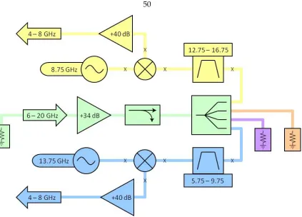
3.4.1 Wideband IF Processor

The IF processor (see Figure 3.15) accomplishes three basic functions: separation into four bands, downconversion to the WASP2 input frequencies, and amplification. Each of the functions is relatively straightforward in principle, but the large bandwidth creates special design concerns. Each WASP2 unit accepts a 3.5-GHz wide input, centered on 6 GHz. The total bandwidth available from the four WASP2 units is 14 GHz, which slightly exceeds the intended IF bandwidth of the receiver. Z-Rex was designed to provide a 12-GHz output from 6 - 18 GHz; however, rather than waste some of the WASP2 bandwidth, we chose to design a downconverter to accept a slightly broader input, thereby providing an easy mechanism for taking advantage of any extra output range from the receiver. The input spectrum is thus divided into four slightly overlapping bands: 5.75 - 9.75 GHz, 9.25 - 13.25 GHz, 12.75 - 16.75 GHz, and 16.25 - 20.25 GHz. Each band is downconverted to a 4 - 8 GHz output. If the WASP2 spectrometers have exactly the quoted 3.5-GHz bandwidth, these ranges will precisely tile the range from 6 - 20 GHz. Any extra input bandwidth offered by the WASP2s allows the spectra to overlap lightly. The four branches are summarized in Table 3.2.

The downconversion also requires appropriate component selection. The choice to ex-tend the frequency coverage to 20 GHz (rather than 18 GHz) requires high-performance components. The 5.75 - 9.75 GHz band provides additional challenges, as the RF input overlaps the desired IF output. Discussions with vendors indicated that a triple-balanced mixer would be appropriate for that branch, as such mixers are particularly good at mini-mizing RF-to-IF leakage. Further investigation revealed that triple-balanced mixers would be needed for all four bands, as the 4 - 8 GHz output is beyond the range of double-balanced mixers designed for similar RF frequencies.

(56)

Figure 3.11: Experimental set up for measuring port-to-port mixer isolation. The DRO (left) was connected to the LO port of the mixer via a 3-dB attenuator. To measure LO-to-RF isolation, the IF port was loaded with a 50-Ωterminator, and the RF port was connected to a spectrum analyzer via a short (∼ 12”)cable with a 10-dB attenuator at the end (blue labels). LO-to-IF isolation was measured by terminating the RF port and connecting the IF port to the spectrum analyzer (red labels). Reference measurements were taken by remov-ing the mixer and measurremov-ing the output of the DRO through the remainremov-ing elements.

Triple-balanced mixers are readily available commercially, but they typically have worse port-to-port isolation than their double-balanced counterparts. Since our design includes LO sources within the input band, isolation is also an important criterion for us. To de-termine whether the mixers would work for our needs, we directly tested the isolation using the experimental setup shown in Figure 3.11. We paired each mixer with all four LO sources to determine its LO-to-RF and LO-to-IF isolation at the frequencies of interest, generating the results given in Table 3.1.

(57)

LO-to-RF Isolation (dB) LO-to-IF Isolation (dB)

DRO Frequency (GHz) DRO Frequency (GHz)

Mixer 8.75 12.25 13.75 17.25 8.75 12.25 13.75 17.25

M3006L 0247A 26.5 18.8 22.9 35.6 23.8 27.3 23.1 30.1

M3006L 0247B 29.2 20.6 25.0 37.0 27.4 21.2 21.3 37.5

M3006L 0247C 22.5 29.0 23.2 28.1 27.5 16.6 15.6 32.8

M3006L 0247D 26.7 21.6 25.6 32.4 31.0 26.9 35.1 30.6

M3006L 0247E 25.3 22.4 27.4 32.5 38.8 20.9 28.2 42.7

M2H-0220LA 27.7 45.1 44.7 30.1 22.3 32.0 29.1 27.3

Table 3.1: Mixer isolation, measured using the setup shown in Figure 3.11. The M3006L 0247X lines represent different units from Advanced Microwave while the final line corre-sponds to Marki Microwave M2H-0220LA.

3.4.1.1 Prototype and Spur Analysis

To determine whether the in-band LO sources would generate spurious spikes in the out-put signal, a two-branch prototype of the IF processor was built, as shown in Figure 3.12. In the prototype, the input signal, shown by the green arrow, was amplified, passed through a coupler, and then split by a four-way power divider. Two of the outputs from the divider were terminated, while the other two outputs fed into 4-GHz-wide bandpass filters. Each of these bands was then downconverted into the 4 - 8 GHz band and amplified. All parts were the same as the ones described in the final IF processor design in Section 3.4.1.3.

These two branches were chosen because they offered particularly strong tests of the mixers’ isolation; the RF input for the 5.75 - 9.75 GHz branch overlapped with the IF out-put, and the 8.75-GHz LO of the other branch fell near the edge of the input bandwidth for the final 4 - 8 GHz amplifier. The best mixers were picked for each branch based on the results found in Table 3.1. The 5.75 - 9.75 GHz branch also allowed us to study the high-frequency behavior of the bandpass filters, which was also a source of concern.

(58)

Figure 3.12: Simple two-branch prototype of the IF processor. X’s indicate 3-dB attenua-tors.

5.75 - 9.75 GHz branch demonstrated the latter behavior, providing a good test of whether this high-frequency leakage would allow unintended interactions between bands.

The entire range of the spectrum analyzer, from 0 - 26.5 GHz, was searched for peaks; particular attention was given to 5 GHz and 22.5 GHz since mixing between the fundamen-tal frequencies of the LO sources would be expected to yield peaks at those frequencies. Since the LOs themselves were the sources of interest, the input to the broadband amplifier was terminated, as was the output of whichever line was not connected to the spectrum analyzer.

For the 5.75 - 9.75 GHz line, peaks were found at 3.75 GHz and 13.75 GHz; no peaks were found at 5 or 22.5 GHz. The 13.75-GHz peak’s power and frequency were consistent with the LO leaking through to the IF. The 3.75-GHz peak could best be explained by the second harmonic of the 8.75-GHz LO mixing with the fundamental of the 13.75-GHz LO (2×8.75−13.75=3.75 GHz).

(59)

(60)

the fundamentals of the LO sources, and the 8.75-GHz peak was consistent with LO-to-IF leakage. The 17.50- and 26.25-GHz lines represented the second and third harmonics of the LO frequency; presumably, they were due to frequency multiplication in the mixer and/or amplifier. To determine which element was causing the multiplication, the amplifier was removed, and the spectrum analyzer was connected to the 3-dB attenuator on the IF port of the mixer. The 17.50-GHz peak dropped by only a few dB, implying that the mixer was at least partially responsible for the frequency doubling. In contrast, the 26.25-GHz peak dropped by ∼ 20 dB, indicating that it was most likely caused by frequency multiplica-tion within the amplifier. This can happen when a particularly strong line saturates the amplifier, forcing it into a nonlinear regime.

Further tests were done to try to rule out other sources of interaction (such as LO fre-quencies leaking through the ground plane or DC wiring), but all tests were consistent with the interpretations given above. In the case of the 3.75-GHz peak, it was possible to trace the hypothesized 17.5-GHz line through much of the system. It was found at the RF port of the mixer on the 12.75 - 16.75 GHz branch, supporting the idea that it was caused by LO-to-RF leakage. The same line could be found at the output of the power splitter sending signals into the 5.75 - 9.75 GHz branch. From there, the signal disappeared below the noise floor of the spectrum analyzer.

Experiments with the prototype system yielded several important insights for moving forward on the final design. It demonstrated that interactions between LOs could generate spurs and that higher-order interactions would need to be considered as well. These in-teractions were not symmetric; the 5-GHz peak could be detected in the 12.75 - 16.75 GHz branch, but not in the 5.75 - 9.75 GHz branch, presumably because the two LO signals encountered different losses in the bandpass filters as they worked through the system. Fi-nally, the frequency multiplication of the 8.75-GHz LO indicated that the output amplifiers could be saturated by strong out-of-band spurs; adding a broadband 4 - 8 GHz bandpass filter would resolve this problem.

(61)

order), and calculates the sum and difference frequencies generated by the two signals. In addition, it calculates the attenuation encountered by each signal as it works its way upstream in one branch and then back down through a different branch using laboratory measurements of the bandpass filters’ performance taken with a 40-GHz network ana-lyzer. Whenever a mixing product is found that falls within the output band of the IF processor, the program reports the frequency of the spur and the expected attenuation of the underlying signal.

The program accurately predicts the spurs that were observed with the prototype, and predicts that the 3.75-GHz spur should be significantly stronger in the 5.75 - 9.75 GHz line, as was seen. It also finds other potential spurs that were not identified with the prototype, but attaches higher attenuation values to them.

In addition to modeling the existing filters, the program also allowed us to study the effects of adding new filters. We