Label-free Detection of Single Molecule Using Microtoroid Optical Resonators

(1)

Label-Free Detection of Single Biological Molecules Using

Microtoroid Optical Resonators

Thesis by

Judith Su

In Partial Fulﬁllment of the Requirements

for the Degree of

Doctor of Philosophy

California Institute of Technology

Pasadena, California

2014

(2)

Judith Su

(3)

(4)

Abstract

Being able to detect a single molecule without the use of labels has been a long standing goal of

bioengineers and physicists. This would simplify applications ranging from single molecular binding

studies to those involving public health and security, improved drug screening, medical diagnostics,

and genome sequencing. One promising technique that has the potential to detect single molecules

is the microtoroid optical resonator. The main obstacle to detecting single molecules, however, is

decreasing the noise level of the measurements such that a single molecule can be distinguished from

background. We have used laser frequency locking in combination with balanced detection and data

processing techniques to reduce the noise level of these devices and report the detection of a wide

range of nanoscale objects ranging from nanoparticles with radii from 100 to 2.5 nm, to exosomes,

ribosomes, and single protein molecules (mouse immunoglobulin G and human interleukin-2). We

further extend the exosome results towards creating a non-invasive tumor biopsy assay. Our results,

covering several orders of magnitude of particle radius (100 nm to 2 nm), agree with the ‘reactive’

model prediction for the frequency shift of the resonator upon particle binding. In addition, we

demonstrate that molecular weight may be estimated from the frequency shift through a simple

formula, thus providing a basis for an “optical mass spectrometer” in solution. We anticipate

that our results will enable many applications, including more sensitive medical diagnostics and

fundamental studies of single receptor-ligand and protein-protein interactions in real time. The

thesis summarizes what we have achieved thus far and shows that the goal of detecting a single

(5)

List of Figures

1.1 Biosensing with a Biacore surface plasmon resonance instrument . . . 3

1.2 The microtoroid as an example of a whispering gallery mode optical resonator. . . 4

1.3 Response trace for a microtoroid WGM resonator. . . 7

1.4 Dose response curves for protein A binding to human Fc fragments. . . 7

2.1 Toroid fabrication ﬂow stream . . . 11

2.2 SEM micrograph of an array of microtoroids. . . 12

2.3 Eﬀect of the ﬂat top laser beam shaper . . . 13

2.4 CO2 laser schematic . . . 13

2.5 CO2 laser setup photographs . . . 14

2.6 Taper puller schematic and photograph . . . 16

2.7 Testing setup schematic . . . 17

2.8 Testing setup pictures . . . 18

2.9 Schematic of microtoroid aligned with optical ﬁber . . . 19

3.1 Overview of a conventional scanning method . . . 21

3.2 Overview of Frequency Locked Optical Whispering Evanescent Resonator (FLOWER). 22 3.3 An overview of the frequency locking method for peak tracking . . . 23

3.4 Block diagram of how a resonance peak is located (path shown in red). . . 24

3.5 Sequence of operations how the quality factor of a microtoroid is measured over time. 25 3.6 Block diagram of toroid control system. . . 27

(9)

3.8 Conceptual basis for how the error signal is generated. . . 29

3.9 Block diagram of PID control. . . 31

3.10 Output of the Mach-Zehnder interferometer . . . 32

3.11 Tracking the resonance peak of the toroid in response to heating. . . 34

3.12 Noise level of system before frequency locking is implemented . . . 35

3.13 Noise level of system after frequency locking is implemented . . . 36

3.14 Noise level of system after frequency locking is implemented . . . 38

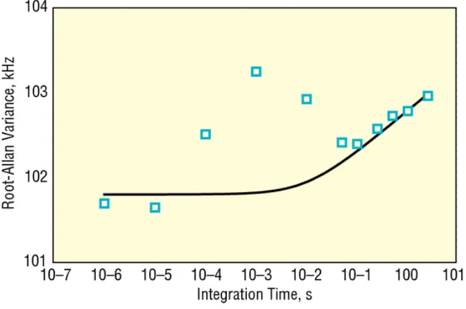
3.15 Laser linewidth as function of integration time . . . 39

3.16 System Bode plot. . . 40

4.1 Data processing overview . . . 42

4.2 Data processing ﬂow chart . . . 43

4.3 Time trace of ﬁltered data set . . . 44

4.4 Filtering a raw data set (blue) in frequency space . . . 45

4.5 The plateau region of a step has a slight slope . . . 46

4.6 Zoomed in comparison between frequency ﬁltering methods . . . 48

4.7 Median ﬁlters of varying window sizes being applied . . . 49

4.8 Data after a median ﬁlter of 1001 has been performed . . . 50

4.9 Total variation denoising algorithm run for a variety of diﬀerentλ. . . . 52

4.10 A zoom-in of the total variation denoising algorithm run for a variety of diﬀerentλ . 53 4.11 Total variation denoising algorithm shown with onlyλof 5×10−4. . . 54

4.12 A comparison of TVD results with median ﬁlter results. . . 54

4.13 Outline of step ﬁtting algorithm . . . 56

4.14 Outline of step ﬁtting algorithm (cont’d) . . . 57

4.15 Step ﬁts and histograms with various ﬁlters applied . . . 59

4.16 Histograms created from data processed just a linear ﬁlter . . . 60

4.17 Histograms created from data processed with a median ﬁlter. . . 61

(10)

4.19 TVD histograms with Gaussian curve overlays. . . 63

4.20 Step number step ﬁt quality curves for linearly, median, and TVD ﬁltered data . . . . 63

4.21 Step duration step ﬁt quality curves for linearly, median, and TVD ﬁltered data . . . 64

4.22 Step amplitude step ﬁt quality curves for linearly, median, and TVD ﬁltered data . . 64

4.23 Step ﬁt quality plot for pure buﬀer. . . 65

4.24 Histograms created for pure buﬀer data. . . 65

4.25 Step-finding algorithm finds no significant steps for a sloped line with random noise. . 66

4.26 Eﬀect of median ﬁlter on time resolution. . . 67

4.27 Sample cell schematic . . . 69

4.28 Bead detection comparison before and after frequency locking. . . 70

4.29 Detection ofr= 100 nm beads in water. . . 71

4.30 Bead detection data . . . 72

4.31 r= 10 nm particle detection data at diﬀerent powers . . . 73

4.32 Summary of bead detection data. . . 74

5.1 Linker schematic . . . 76

5.2 Fluorescent images of linker binding . . . 77

5.3 FITC-Fc binding to the microtoroid’s surface (no linker) . . . 78

5.4 XPS data demonstrating linker binding. . . 79

5.5 Surface microRaman spectroscopy results . . . 80

5.6 Model of ribosome complex from Saccharomyces cerevisiae . . . 81

5.7 Individual ribosome detection . . . 82

5.8 Exosome cartoon . . . 83

5.9 Exosome detection using the microtoroid . . . 85

5.10 Exosome detection for a non-invasive tumor biopsy assay. . . 86

5.11 Step detection of individual exosomes . . . 87

5.12 Compiled exosome detection results from mice with tumors implanted. . . 88

(11)

6.1 Structure of human IL-2 . . . 93

6.2 Structure of an intact IgG2a monoclonal antibody . . . 93

6.3 IL-2 detection data scales with concentration. . . 95

6.4 Time trace for mouse IgG. . . 97

6.5 Summary of particle detection by FLOWER. . . 98

6.6 Individual human interleukin-2 (2 nm radius) detection. . . 98

6.7 IL-2 detection data at three diﬀerent concentrations . . . 99

6.8 Summary of particle detection data. . . 100

6.9 Maximum wavelength shift may be used to predict mass. . . 101

A.1 Schematic of toroidal integration with microﬂuidics . . . 105

A.2 Photographs of a microtoroid and optical ﬁber inside a microﬂuidic device . . . 105

A.3 Creating microtoroids optimized for mode splitting. . . 106

(12)

List of Tables

4.1 Maximum step amplitude histograms . . . 62

5.1 Mouse tumor data: Fit parametera(steady state value, fm) . . . 86

5.2 Mouse tumor data: Fit parameter 1/b(rise time (s)) . . . 87

5.3 Mouse tumor data: Initial slope (ab) . . . 87

5.4 Nanosight data: Total number of particles/mL . . . 91

6.1 IL-2 binding data: Initial slope (fm/s) . . . 96

6.2 IL-2 binding data: Q-value . . . 96

(13)

Chapter 1

Introduction

1.1

Biological and chemical sensing using microtoroid optical

resonators

Highly sensitive biodetection is important for many applications such as high throughput drug

discovery studies, as it can dramatically reduce the amount of analyte needed and speed the assays.

A variety of applications in medical diagnostics (e.g., detecting trace amounts of tumor speciﬁc

antigens to monitor the re-occurrence of cancer) and public health (e.g., detecting bacteria or viruses)

would beneﬁt from improved speed and sensitivity [1]. If the sensitivity can be pushed to the single

molecule level, fundamental studies become more direct and decisive, permitting, for example, studies

of molecular conformations at a single molecule level [2]. Since the early reports in the mid-70’s

[3], label-mediated single-molecule detection has become routine in many laboratories. Certain

biophysical events, such as, the action of molecular motors (myosins and kinesins) are best studied

from a single molecule viewpoint. Basic features, such as the motor’s step size, would be obscured

by the averaging from traditional bulk measurements.

Biosensing techniques can be separated into two categories: those that require labeling of the

target molecule (e.g., by attaching some ﬂuorescent [4], radioactive [5], or enzymatic tag), and those

that are label-free, sensing directly some physical property of the analyte. The majority of single

molecule studies have required labels, using a bead or dye on a molecular motor to follow its motion

(14)

diﬃcult to generate, and for small analytes, might perturb the molecular events under study. One

of the most commonly used label-free tests is, the ELISA, which senses an analyte via its binding

to an antibody. In recent years, there has been a push towards the development of sensitive

label-free techniques, resulting in a range of new ultra-sensitive techniques including optical microcavities

[6, 7], mechanical sensors such as cantilevers [8, 9], and electrical sensors such as nanowires [10]

and ion-sensitive ﬁeld-eﬀect transistors (ISFETs) [11]. The current gold standard for label-free, low

concentration biosensing is the Biacore [12], an instrument ﬁrst commercialized in 1990 that has

since received over 1200 citations, attesting to its utility and popularity. The Biacore’s operation

is based upon surface plasmon resonance [12, 13], sensing the binding of an unlabeled analyte to a

cognate receptor that has been covalently bound to a thin metal surface. The analyte binding is

measured as the deﬂection of a laser bounced oﬀ the metal-solution interface, because the change

in the index of refraction from the analyte alters the manner in which the plasmon waves of the

metal substrate’s surface interact with the evanescent light. While this sensing mechanism is

label-free, the Biacore is not highly sensitive. It requires that enough analyte binds to alter the index of

refraction over the region of the laser illumination. As a result, the typical lower limit of detection

of the Biacore is on the order of nM in∼250µl of solution (Figure 1.1), several orders of magnitude greater than the typical of the single molecule regime (∼attomolar concentrations).

Recently a class of devices known as whispering gallery mode (WGM) optical resonators has

attracted attention due to their potential for ultra-sensitive biological and chemical detection. These

devices are named after the whispering gallery acoustical eﬀect discovered by Lord Rayleigh while

standing under the dome in St. Paul’s cathedral in London. Whispers at one end of the dome could

be heard at the other end due to the sound reﬂecting along the edges of the dome with low loss

[14]. Whispering gallery mode optical resonators operate based on light circulating inside a glass

device. The ﬁgure of merit for these devices is known as the quality factor (Q), deﬁned as the ratio

of the resonant wavelength (λ), to its linewidth (∆λ). Q is proportional to how many times the light

(15)

Figure 1.1: Biosensing with a Biacore surface plasmon resonance instrument.(A) The binding of analytes to covalently attached binding partners (i.e., antibodies or receptors) changes the index of refraction near the metal film and changes the angle of the reflection. As the change in index of refraction requires no exogenous label, and is proportional to the amount of analyte bound, the magnitude and rate of deflection provide a simple means to obtain quantitative data on binding. (B) Biacore response plot (sensorgram) of biotinylated-protein G binding to streptavidin (linked to the sensor chip). A half log dilution series was preformed from micromolar down to attomolar concentrations. The minimum detectable response was 3.16 nM. Traces from smaller concentrations spanning nine orders of magnitude superimpose as the lowest trace and are indistinguishable from noise.

ﬂuid, permitting a Biacore-like sensing of an analyte bound to the surface. Because these devices

are made of glass they can be functionalized to allow for the speciﬁc attachment of “bait” molecules.

When analyte molecules bind to the bait this causes a change in the index of refraction near the

device, which in turn alters the resonance frequency (Figure 1.2). The high Q contributes to the

sensitivity in two ways: ﬁrst, the light circulates in a small mode volume over 250,000 times,

re-interrogating any bound analyte many times; second, the high Q value gives a narrow resonance

peak, whose wavelength can be measured accurately.

The most widely used of these optical resonators for biosensing are the microsphere [15–24],

microring [25–42], and microtoroid [43–48], so named because of their geometries. Due to the heat

reﬂow (melting) treatment designed to remove surface imperfections, microspheres and microtoroids

possess an extremely (atomic scale) smooth surface ﬁnish [44], and thus retain light for longer (on the

order of tens of nanoseconds) periods of time. Microrings retain the lithographic blemishes caused

during manufacturing; however, they can be fabricated in conjunction with a waveguide to input

light (as opposed to microspheres and microtoroids that require critical positioning of a tapered

(16)

Figure 1.2: The microtoroid as an example of a whispering gallery mode optical resonator. (A) A scanning electron micrograph of a microtoroid. (B) A schematic of the evanescent wavefront interacting with molecules near the microtoroid (not to scale) (C) Molecules binding to the toroid’s surface changes the resonant frequency of the device. Whispering gallery mode resonators provide enhanced sensitivity as light interacts with the analyte molecules multiple times.

to perform many experiments simultaneously on a large scale. To date, microspheres have been

shown capable of detecting a single nucleotide polymorphism in a µM of solution [22] as well as a single InfA virus [15] and microrings have been used to simultaneously detect 5 diﬀerent protein

markers with picomolar sensitivity [49].

Compared to microspheres and microrings, microtoroids are likely to have the greatest sensitivity

[44]. Microtoroids have demonstrated 100 times higher quality values in water [50] and have smaller

mode volumes than microspheres, which should increase sensitivity by increasing the number of

times light circulates and by concentrating more light in a smaller volume. In addition, the toroids

have fewer propagation angles than a sphere, and they are easier to mode match to the optical ﬁber

taper, maximizing the size and sharpness of the drop in transmission of the optical ﬁber that appears

at the WGM resonance (Figure 1.2).

Extremely high sensitivity was demonstrated by Lu et al. [50], who used a Mach-Zehnder

inter-ferometer as a means to more accurately measure the laser wavelength, allowing them to subtract

laser frequency jitter noise from the measured toroidal response signal, thus enhancing sensitivity.

(17)

has a mass of 6 ag, and BSA has a mass of 0.1 ag [21]. We note that detection signal strength scales

with particle volume [18].

In a hybrid dual-resonator approach, microspheres have recently been coupled to 70 nm radius

silica core gold nanoshells to boost signal in order to detect single BSA (∼14 nm) molecules [21], however, this approach is limited in that there are only two hotspots per nanoparticle and one

nanoparticle per microsphere limiting the active detection area of the sensor. The advance described

here, Frequency Locked Optical Whispering Evanescent Resonator (FLOWER), would improve the

detection capabilities of optical resonators in general, including hybrid systems.

1.2

The microtoroid as a viable, quantitative biosensor

To compare the microtoroid [44] as a biosensor with the Biacore, we performed parallel analyses of

the same series of analyte solutions (Protein A) and binding partners attached to the sensors (Fc

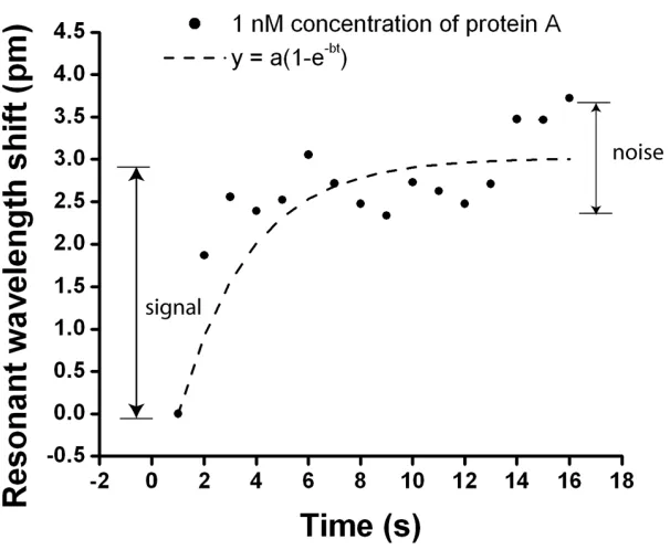
Region of human IgG). An example microtoroid response trace for a 1.0 nM concentration of protein

A shows a measured resonance shift of the toroid with a signal-to-noise ratio (SNR) of >3 in 15 seconds (Figure 1.3), signiﬁcantly faster than the Biacore performance at 3 nM (Figure 1.1B). The

Biacore, and other emerging label-free biodetection techniques such as cantilevers [51], are in general

slower, with steady state response times of up to hours. The fast response times of the microtoroids

oﬀer advantages for applications such as high throughput analyses and medical diagnostics. This

data was taken via the conventional swept-frequency method in which the laser continuously scans

through a range of wavelengths to ﬁnd the resonance wavelength of the microtoroid.

Quantitative parameters such as equilibrium dissociation constants (Kd, the concentration of

analyte that produces a response at half saturation) can be extracted from the microtoroid from

a dose-response curve. For the Biacore, this involves plotting the steady state beam deﬂection for

a series of concentrations; for the microtoroids this involves plotting the steady state resonance

wavelength shift. Figure 1.4 compares the dose-response curves for the Biacore and microtoroid

sensors, using the same Protein A-IgG interaction pair as used in Figure 1.3. Good agreement of the

(18)

the sparse (N = 1) data set. Interestingly, the dose-response curve of the toroid is steeper (Hill

(19)

Figure 1.3: Response trace for a microtoroid WGM resonator. The resonance wavelength shifts within seconds to a new value after a 1 nM solution of protein A is flowed onto a toroid functionalized with the Fc region of human IgG. The response to the flow rate of 50µl/min is fit adequately by a simple exponential (r2 _{= 0.7).}

A

B

(20)

1.3

What is the true limit of detection? The single molecule

controversy

In 2007, a paper was published by in Science [52] claiming to have detected single molecules using the

microtoroid, however, this result was met with considerable skepticism [27, 53–55]. In this report, an

antibody directed against interleukin-2 was non-speciﬁcally bound to the surface of the microtoroid

and a low concentration of interleukin-2 was ﬂowed by. Sudden, step-like changes in resonance

wavelength were taken to be the response of the microtoroid to single molecules. As expected, the

rate of these events linearly scaled with concentration (but the amplitude did not) and followed

Poisson binding statistics in time as would be expected for single molecule detection. In addition,

an experiment was performed in which ﬂuorescently tagged molecules were bound to the microtoroid

so that their unitary photo-bleaching could be used to “count” molecules. Unitary blue shifts in

the resonance wavelength and corresponding increases in the quality factor of the microtoroid were

seen, as anticipated when particles with large absorption cross-sections bleach or un-bind from the

microtoroid.

In support of these experiments, a thermo-optic model was proposed to explain the step-like

shifts from single molecules binding [52]. The thermo-optic theory proposed that the local heating

of the toroid would result from the large circulating power interacting with single molecules bound

to the toroid. The temperature dependence of the index of refraction would thereby amplify any

wavelength shift as single molecules bound to the toroid. The molecular cross-sections used to

calculate the expected shifts from a single molecule, however, were recorded as more than a factor

of a 1000 too large, calling into question the reported match between experiment and theoretical

prediction [54, 56]. As stated in [54]:

(21)

Thus, the model as developed in [52] does not predict the experimentally observed steps, given

the real absorbance cross sections. A correction was later published retracting the model [57]. As a

further point of controversy, the results have yet to be repeated [53, 55].

Linear theory suggests that the shift is dependent purely on index of refraction changes in the

evanescent ﬁeld due to the binding of a molecule, and not on the quality factor of the toroid or

laser power [54]. Arnold, et al., computed the ratio of the contribution from the linear reactive

mechanism to the thermo-optic mechanism for both a sphere and a toroid and found that the

contribution from the thermo-optic mechanism should only be 40% of the linear mechanism, and

not several thousand times larger as was initially predicted [52]. Therefore, we expect the observed

shift to be approximately predicted by the linear mechanism alone by at least within a factor of 2.

This greatly simpliﬁes the model.

Questions have also been raised regarding the high binding rate of molecules to the microtoroid’s

surface. Squires et al., [51] modeled based on pure diﬀusion what the time between binding events

should be and arrived at an estimate of one event every six to seven seconds for a molecule of

diﬀusivityD= 10µm2_{/s and a concentration of 10 fM. Furthermore, Squires et al., calculated that} equilibrium should take around one hour to reach. Recent work by Arnold, et al., has shown that

microspherical optical resonators generate optical trapping forces that cause signiﬁcantly enhanced

(100×) nanoparticle transport velocities [58]. We anticipate this eﬀect to be even greater in our frequency-locked system as we are always on resonance as opposed to sweeping past resonance, thus

increasing the amount of circulating power our devices experience. This signiﬁcantly increases the

expected particle encounter rate. Our rates are consistent with the binding rates from nanowire

experiments which report saturation from the binding of thousands of molecules within seconds at

similar concentrations [10]. We note that the binding rates from our experiments and from nanowire

experiments are dramatically faster than the mass transport predicted by Squires et al. A full

analysis of the mass transport in this system remains unavailable, and the discrepancy between

(22)

Chapter 2

Microtoroid creation and

experimental setup overview

2.1

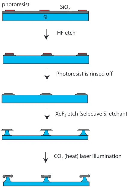
Toroid fabrication

Microtoroids are fabricated using a combination of lithography and etching techniques [44]. An

overview of this process may be seen in Figure 2.1. First, circular pads of photoresist are patterned

on top of a silicon wafer with a 2 micron thick thermal oxide layer. After patterning, the areas

in between the circular pads are etched away using hydroﬂuoric acid, leaving behind a silicon pad

with an SiO2 top. The silicon pad is selectively undercut using XeF2 etching to form a pillar. This

structure is known as a microdisk. To generate an atomically smooth surface ﬁnish, the microdisk is

melted or reﬂowed using a CO2 laser. This process collapses the microdisk into a smooth structure

known as a microtoroid. To further ensure high quality factors, we used intrinsic silicon wafers.

These wafers have been doped with a less than typical amount of Boron. The presence of Boron

lowers the index of refraction of the microtoroid and has been shown as a result to lower the quality

(23)

Si

SiO2

photoresist

HF etch

Photoresist is rinsed off

XeF2 etch (selective Si etchant)

CO2 (heat) laser illumination

(24)

Figure 2.2: SEM micrograph of an array of microtoroids. Toroids are fabricated on a silicon wafer following the procedures of [44]. Toroid fabrication was performed using the cleanroom facilities at the Kavli Nanoscience Institute (KNI), Caltech.

2.2

Modiﬁcation of CO

2

laser reﬂow system

One signiﬁcant challenge in creating microtoroids, is the successful creation of microtoroids with

ultra-high (>108) quality factors. This requires extremely uniform heating of the toroid when it

is in the microdisk stage. To improve our yield of ultra-high-quality microtoroids, we implemented

a ﬂat top laser beam shaper (Edmund Optics) made out of ZnSe that converts the Gaussian laser

beam input from our CO2 laser to a collimated ﬂat output beam. As shown in Figure 2.3, the ﬂat

top laser beam shaper provides more uniform illumination and therefore a more uniform reﬂow of

the microdisk. A schematic of the CO2 laser reﬂow system may be seen in Figure 2.4. Because the

wavelength of the CO2laser light (10.6µm) is invisible to the human eye, the laser was ﬁrst aligned using a Helium Neon laser at 633 nm. Some photographs of the setup are shown in Figure 2.5.

(25)

generator to the CO2 laser.

A

B

Figure 2.3: Uniform illumination of the microdisk allows for a symmetric toroidal structure to be created. To aid in this process, a flat top laser beam shaper was used. The effect of the flat top laser beam shaper may be seen by shooting the CO2 laser beam at a glass coverslip and looking at the shape of the melted glass. As shown in (A), before the addition of the beam shaper the beam spot is non-circular while as shown in (B), after the addition of the beam shaper the beam spot is very circular and uniform.

CO₂ laser

flat top laser beam shaper

ZnSe plano convex lens ZnSe mirror

CCD

sample plane HeNe laser

mirror (flipped down during reflow process)

alignment laser _{beam steering mirrors}

pinhole

ZnSe beam combiner

(26)

CO2 laser

HeNe laser ZnSe mirror

Flat top laser beam shaper pinhole

Plano-convex focusing lens

ZnSe beam combiner

Sample holder HeNe

1

Figure 2.5: CO2 laser reﬂow system photographs. As shown in the photographs, the CO2 laser was hard mounted onto an air ﬂoated optical table for stability. The beam was steered using ZnSe mirrors and aligned through two pinholes. Finally, the beam was focused onto the microdisk sample using a plano-convex ZnSe lens. For visualization purposes a beam combiner which passes light at

10.6µm and reﬂects light at 633 nm was placed before the sample so that the visible light could be

reﬂected through an imaging column and towards a camera.

2.3

Optical ﬁber pulling setup

There are several ways of coupling light into microresonators, including direct illumination, prism

coupling, and tapered optical ﬁber coupling. Of these, we use evanescent coupling from a tapered

optical ﬁber because of its low loss [60–62]. In a typical optical ﬁber, the cladding and large diameter

of the ﬁber prevents evanescent light from leaking out of the ﬁber. In our case, we want the evanescent

mode to leak out from the part of the ﬁber adjacent to the toroid. This can be easily achieved by

removing the cladding from the ﬁber in this region and by pulling on the ﬁber to shrink its diameter

in this region. When the ﬁber’s diameter is on the order of or smaller than the optical wavelength,

a significant amount of optical power is carried in the evanescent field of the fiber. When the toroid

is brought within this evanescent ﬁeld, light naturally couples from the ﬁber to the toroid and back

again. It is important to develop a repeatable method for thinning the ﬁber in a small region, which

(27)

Brieﬂy, a spool of single mode optical ﬁber was purchased from Newport and about a meter was

unwound. One end of the spool was ﬁber coupled into the laser, while a 1 cm portion of cladding

was removed from the middle of the unwound section. Removing the cladding changes the index of

refraction of the optical ﬁber making it multi-mode, so the optical ﬁber is simultaneously thinned

and pulled until it can only support one mode again. The ﬁrst step in this procedure is washing the

portion of the optical ﬁber that has had the cladding removed with isopropanol alcohol and clamped

on either end with magnetic clamps. The assembly was mounted above a hydrogen torch and the

ﬁber was simultaneously heated and pulled in opposite directions at 60µm/min using two stepper motors (Edmund Optics). To make the heating and thus the thickness of the optical ﬁber more

uniform, the hydrogen torch was dithered horizontally (Figure 2.6(a) and Figure 2.6(b)) at 1 Hz.

Pulling was stopped when the ﬁber became single mode (i.e., when the core diameter reduced to a

diameter at which only one mode of light propagation was supported). This was visually estimated

to occur when the laser light through the optical ﬁber stopped blinking and therefore we could

conclude that significant intensity fluctuations had stopped. The end of the optical fiber was then

cleaved and inserted into an auto-balanced photodetector using a bare ﬁber adapter. A typical waist

(28)

stepper motor

stepper motor optical fiber

hydrogen torch (dithered horizontally at 1 Hz)

(a) Optical ﬁber taper puller schematic.

hydrogen torch

motor controller CCD

viewing microscope

stepper motor stepper motor

motor to dither torch

taper holder taper

(b) Optical ﬁber taper puller picture.

Figure 2.6: (a) Schematic of the optical fiber taper puller. To thin the optical fiber sufficiently such that the majority of the light is carried evanescently, the optical fiber is heated using a hydrogen torch and pulled using two stepper motors. To enable more uniform heating of the optical fiber, the hydrogen torch was dithered at a frequency of 1 Hz. (b) Photograph of the optical fiber taper puller. The optical fiber is held in place using a custom machined holder with magnetic clamps. Two stepper motors pull the optical fiber in opposite directions while a hydrogen torch heats the fiber. For visualization purposes, an imaging column with a low (10×) magnification objective and CCD camera is positioned such that a side view of the optical fiber may be seen while pulling occurs.

2.4

Testing setup

Once an optical ﬁber has been pulled, the resonance peak of the microtoroid may be found by

ﬁrst bringing the toroid into close proximity to the optical ﬁber using a three-axis nanopositioner

(Physik Instrumente). The coupling eﬃciency of light into the toroid may be tuned by controlling

the distance between the optical ﬁber and the microtoroid [56]. A schematic of the testing setup

is shown in Figure 2.7. Two imaging columns are placed perpendicular to each other to generate a

top view and a side view image of the microtoroid so that the microtoroid may be visually aligned

(29)

that reﬂects infrared light was placed in front of both imaging light sources. Some photographs of

the setup may be seen in Figure 2.8. A schematic of the toroid positioned in relation to the optical

ﬁber is shown in Figure 2.9.

top illumination

side illumination

nanopositioner

light

ligh

t

CCD

C

CD

50/50 beam splitter

hot mirror

(30)

nanopositioner

3-axis stage

taper holder toroid

fiber spool _{top viewing column}

enclosure to minimize air currents laser

fiber spool

auto-balanced detector

top viewing column

top view side view

(31)

22 mm

1 mm

side view

6.4 mm

optical fiber

top view

inlet syringe

8.4 mm

(32)

Chapter 3

Improving the signal-to-noise ratio

using laser frequency locking

3.1

Introduction

The main hurdle for single molecule detection is improving the signal-to-noise ratio such that the one

molecule can be distinguished from background. Typically with whispering gallery mode resonators,

molecular binding events are detected by continuously scanning the input frequency of a laser using

a function generator and monitoring transmission dips in the optical ﬁber output that occur when

(33)

Oscilloscope Pump (~633 nm)

Histogram of Binding Events Frequency Scanning

Step finding

Figure 3.1: Overview of a conventional scanning method for tracking resonant wavelength shifts using a microtoroid optical resonator. In this system, the wavelength of a tunable laser is continuously scanned through a range of wavelengths using a function generator to locate the resonant wavelength of the microtoroid. The output of the scan is detected using a photodetector and the results are displayed using an oscilloscope.

Once resonance is found, the wavelength trace is recorded and curve ﬁt to ﬁnd the peak. Tracking

the centroid of the peak over time generates a data set to which steps may be ﬁt and a histogram

of binding events may be created. This method takes a long time and has accuracy limited to the

rate (typically 100 Hz for a conventional tunable laser system such as New Focus 6300) and range

at which the laser is being swept.

Our frequency locking approach is an improvement over prior scanning systems that

continu-ally sweep back and forth over a large frequency range (3.1×104 fm, only occasionally matching resonance. In contrast, our work directly tracks the resonant wavelength location within a narrow

and adaptively varied frequency range with a ﬁxed length of 19 fm. Thus we track discrete

ﬂuctu-ations in signal more accurately and quickly, permitting slight and transient events to be detected

(Figure 3.2). Frequency locking feedback control has been used in applications such as in scanning

tunneling microscopy to maintain tip-surface separation [63]; however, to the best of our knowledge

(34)

b a

x +

PID

error signal

laser detector

dither

Time avg microtoroid c

+

x

Wavelength (λ)

T

o

ro

id

re

sp

o

n

se

(d)

We measure the amount the laser shifts to stay on resonance (d)

new location

computer

Figure 3.2: (a) Rendering of a microtoroid coupled to an optical fiber (not to scale). In our system, a frequency-tuned laser beam is evanescently coupled to a microtoroid (∼90 microns in diameter) using an optical fiber (red). At resonance, light (red curved arrow) coming out of the microtoroid destructively interferes with light going straight through the optical fiber (red arrow), causing a dip in the transmission (peak in absorption) vs. light wavelength. (b) Conceptual basis for particle detection. The laser frequency (red solid line) is locked to the resonance frequency of the microtoroid (blue line). As particles bind, the resonant frequency of the microtoroid shifts to a new location (green dotted line). We measure the control signal needed to keep the laser locked to the microtoroids new resonance frequency (red dashed line). (c) Block diagram of the sensing control system. A small high-frequency dither is used to modulate the driving laser frequency. When multiplied by the toroid output and time-averaged, this dither signal generates an error signal whose amplitude is proportional to the difference between the current laser frequency and resonant frequency. This error signal is sent to a PID controller whose output is used to set the laser frequency, thus completing the feedback loop. A computer records the observed frequency shifts.

This approach has two main advantages:

1. Continuously staying on resonance. We are tracking the peak with greater accuracy.

2. Sampling more points per second. We sample at 20 kHz vs. 100 Hz which permits more

averaging. At present, we have achieved millisecond time resolution with the potential for

microsecond time resolution as we are limited only by the speed of our electronics.

3.2

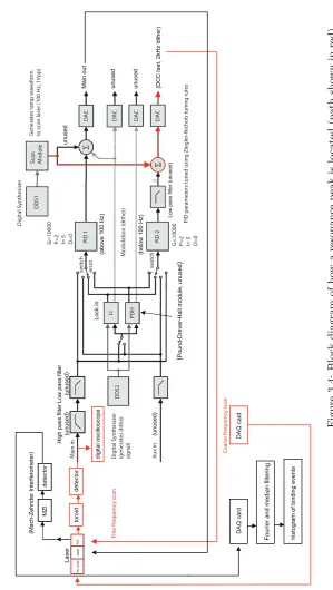
System Overview

Locking the laser frequency to the resonance frequency of the microtoroid is ﬁrst achieved by ﬁnding

the location of the resonance peak by using conventional scanning methods (Figure 3.4). The quality

(35)

Oscilloscope and Balanced Detector Pump (~633 nm)

Histogram of Binding Events Data acquisition card

Feedback controller

Toptica

Computational filtering and step finding Control signal

Figure 3.3: An overview of the frequency locking method for peak tracking. In this system, as op-posed to continuously scanning through a range of wavelengths to locate the resonant wavelength of the microtoroid, a feedback controller continuously tunes the wavelength of the laser to the resonant wavelength of the cavity. By measuring the amount of voltage it takes to keep the wavelength of the laser matched to the resonant wavelength of the cavity, changes in resonant wavelength may be more accurately monitored.

may be determined by curve ﬁtting to a Lorentzian using a custom-written LabVIEW program as

(36)

d io d e H ig h p a s s f ilt e r (unused) L o w p a s s f ilt e r (unused) (D C C I s e t, 2 kH z d it h e r) L o c k i n (u n u s e d ) ( P o u n d -D re v e r-H a ll m o d u le , u n u s e d ) to ro id d e te c to r L o w p a s s f ilt e r (u n u se d ) u n u s e d M Z I (M a c h -Z e h n d e r In te rf e ro m e te r) d e te c to r D A Q c a rd Fouri e r a n d me d ia n f il te ri n g h is to g ra m o f b in d in g e v e n ts (a b o v e 1 0 0 H z ) (b e lo w 1 0 0 H z ) PZ T L a s e r swit ch swit ch er ror Ma in o u t u n u s e d u n u s e d G=10 0 0 0

P=2 I= 5 D=0 _G=10

0

P=2 I= 5 D=0

PID pa ramet ers tun ed usin g Ziegler -N ich ols t un ing rules Dig it a l S yn th esiz er G en er a tes r a mp w a v ef or m to sca n la ser ( 1 0 0 H z, 1 V pp ) Dig it a l S yn th esiz er (gener a tes dith er sig n a l) iz e r G en G en G en G en G en G en G en G en G en to to to sca 0 C oarse fr equenc y scan D A Q c a rd DC mo tor Fine fr equenc y scan d ig it a l o sci llo sco p e M odula tion (dit h er) DDS2

PID 1 PID 2

DDS1

S

can _Module

(37)

Non-linear curve fit to a Lorentzian Max iterations: 10

While Loop

Input signal from A/D card

coefficients matrix Write to spreadsheet

Extract portion of signal

Display of signal and curve fit

Plot of Q value over time

Figure 3.5: Sequence of operations how the quality factor of a microtoroid is measured over time.

After the peak is found, frequency locking is achieved using a lock-in regulator system

(Dig-ilock 110, Toptica Photonics). Brieﬂy, a digital synthesizer generates a dither (sinusoidal external

reference waveform) signal. This dither signal is sent directly to the laser diode which dithers the

frequency over a small range around the resonance peak. This response is detected by a high speed

auto-balanced photodiode (Nirvana, New Focus) and sent to a lock-in error signal generator which

multiplies the modulated signal with the output from the photodiode to create an error signal. An

explanation of why this generates an error signal is given in Section 3.3. The error signal which

repre-sents the diﬀerence between the laser frequency and the cavity resonance, is then minimized by being

sent to two proportional-integral-derivative (PID) feedback controllers. The ﬁrst controller handles

fast (>100 Hz) ﬂuctuations while the second controller handles slow (<100 Hz) ﬂuctuations. These

controllers attempt to match the laser frequency with the cavity frequency by outputting the

appro-priate voltage needed to minimize the error signal. This output voltage is converted to wavelength

(38)

A general overview of the system is presented in Figure 3.6. Although the controller can output a

dither signal up to 10 MHz, in the experiments presented in this thesis, a dither signal of 2 kHz was

used. We note that the dither signal is removed in pre-processing and therefore does not limit the

(39)

d io d e H ig h p a s s f ilt e r (unused) L o w p a s s f ilt e r (unused) (D C C I s e t, 2 kH z d it h e r) L o c k i n (u n u s e d ) ( P o u n d -D re v e r-H a ll m o d u le , u n u s e d ) to ro id d e te c to r L o w p a s s f ilt e r (u n u se d ) u n u s e d M Z I (M a c h -Z e h n d e r In te rf e ro m e te r) d e te c to r D A Q c a rd D ig it a l lo w p a s s f ilt e r H is to g ra m o f b in d in g e v e n ts (a b o v e 1 0 0 H z ) (b e lo w 1 0 0 H z ) PZ T L a s e r swit ch swit ch er ror Ma in o u t u n u s e d u n u s e d G=1 00 00

P=2 I= 5 D=0 _G=1

00

P=2 I= 5 D=0

(40)

3.3

Conceptual Model

An intuitive understanding of how the feedback controller generates an error signal that is sent

to the laser controller may be seen in Figure 3.7. Because the resonance peak (given by L(x) = 1

π

0.5Γ

(x−x0)2+(0.5Γ)2) of the microtoroid is symmetric it is diﬃcult to know on what side of the peak

the laser frequency is located. The derivative of the original signal, however, may be readily used to

locate the center of the peak as it crosses zero at the center and is antisymmetric around the peak.

This makes the derivative a good error signal for the feedback loop as if the laser is to the left of

the peak the error is positive, and if the laser is to the right of the peak, the error is negative. Zero

error is achieved at the top of the peak.

−60 −4 −2 0 2 4 6

0.05 0.1 0.15 0.2 0.25 0.3 0.35

x

L(x)

−6 −4 −2 0 2 4 6

−0.25 −0.2 −0.15 −0.1 −0.05 0 0.05 0.1 0.15 0.2 0.25

L’(x)

x

Figure 3.7: Lorentzian (Γ = 1) and its derivative. The derivative is antisymmetric about the peak

As shown in Figure 3.8, because the toroid response and the dither signal are in phase on the

left side of the peak, the result of the demodulation (multiplying and taking the time average), is

positive. On the right side of the peak, the toroid response and the dither signal are out of phase

(41)

−3

0

−2

−1

0

1

2

3

0.1

0.2

0.3

0.4

x

L(x)

−3

−2

−1

0

1

2

3

−0.2

−0.1

0

0.1

0.2

L’(x)

x

Dither

Toroid response in phase

Toroid response out of phase

error signal negative error signal

positive

Figure 3.8: Conceptual basis for how the error signal is generated. Demodulating (multiplying and taking the time average) the dither signal with the toroid response gives the derivative.

3.4

Symbolic Model

We can show that the error signal is the derivative of the unmodulated toroid response as follows.

Letd(t) = sinω(t) be the dither signal andI =g(λ) be the toroid response to a given wavelength

(42)

v1(t) = βg(λ)≈β

[

g(λ0) + ∂g

∂λ

λ=λ0

(λ−λ0)

]

= β

[

g(αv0) +¯ ∂g ∂λ

λ=αv¯0

(αv0−αv0)¯

]

,

(3.1)

where the central wavelength, λ0, for the Taylor expansion was chosen to be αv0, where ¯¯ v0 is the time average ofv0 over times somewhat longer than the period of the dither signal. The reason for this will become clear shortly. Asv0(t) =d(t) +e(t),we have ¯v0=e(t).

The lock-in ampliﬁer is designed to generate an error signal based on the time average of the

product of the dither signal and the measured photodiode signal:

e(t) = ⟨d(t)·v1(t)⟩

=

⟨

sinω(t)β

(

g(αe(t))) + ∂g

∂λ

λ=αe(t) αsinω

)⟩

=

⟨

βg(α(e(t))) sinωt+αβ ∂g

∂λ

λ=αe(t) sin2ωt

⟩

= 0 +

⟨

αβ ∂g

∂λ

λ=αe(t)

(

1

2−cos 2ωt

)⟩ =1 2αβ ∂g ∂λ

λ=αe(t)

(3.2)

Thus, the error signal generated by the lock-in ampliﬁer is indeed proportional to the derivative of

the unmodulated toroid response,∂g/∂λ.

3.5

PID Control

PID controllers are the most common feedback control system [65]. They are designed for a system

to reach a setpoint as quickly as possible by outputting a control signalu(t) based on the following three component algorithm:

u(t) =kpe(t) +ki ∫ t

0

e(τ)dτ+kd

de

(43)

where,e(t) is an error signal, andkp,ki, andkdare tuning parameters that represent proportional

gain, integral gain, and derivative gain, respectively. This is represented in block diagram form in

Figure 3.9.

PID 1 + 2

e(t)

P

I

D

Σ

PID out

+

Figure 3.9: Block diagram of the PID feedback controller. The error signal from the lock-in regulator is sent to the PID controller. The contributions from the P, the I, and the D, components are multiplied by the error signal and summed to give a signal that causes the controller to reach its set point in a quick and stable way.

Proportional gain produces an output that is proportional to the error, integral gain produces

an output that is proportional to the integral of the error and derivative gain produces an output

that is proportional to the derivative of the error. In this way, proportional gain takes care of the

present error, integral gain takes care of past errors, and derivative gain attempts to predict future

errors through linear extrapolation by calculating a slope.

The values for the PID controllers are set by using a heuristic known as the Ziegler-Nichols

tuning rules that help the system stabilize as quickly as possible. Essentially the overall gain of

the controller is increased until the system oscillates. The gain at which this occurs is denoted as

Ku and the period of oscillation of the system is denoted asTu. The values for proportional gain,

integral time, and derivative time are then given as follows: kp = 0.6Ku, ki= 0.6Ku/(0.5Tu), and

kd= (0.6Ku)(0.125Tu) [65]. The rise and settling times for our system were characterized by sending

(44)

3.6

Converting voltage to wavelength using a Mach-Zehnder

interferometer

The voltage the feedback controller sends to the laser controller to adjust the wavelength of the laser

may be converted to a wavelength using a calibration factor determined from the distances between

fringes of a ﬁber Mach-Zehnder interferometer (MZI). A MZI was created by splitting the output

of the laser into two paths using a 50/50 visible coupler (New Focus). A delay was added in one of

the paths by adding an additional ﬁber that was several meters long. The output was recombined

using another 50/50 coupler and sent to a photodiode whose output was displayed on an oscilloscope

screen (Figure 3.10). As the laser frequency changes as the laser piezo voltage is being swept, the

output of the MZI changes in a fringe sinusoidal pattern. One can compare how much voltage is

put on the piezo with how the laser frequency changes by counting the fringes.

∆λ

(45)

The fringe spacing may be calculated as follows: Let ∆z be the diﬀerence in length between

the two fibers. A peak occurs if ∆z=Nλ_n, whereN is an integer number,nis the fiber refractive index andλis the free space wavelength of the light carried by the optical fiber. Therefore, the free spectral range is:

∆λ = λN−λN+1 = n∆z

N −

n∆z

N+ 1

= n∆z(1

N −

1

N+ 1)

= n∆z( 1

N2_{+ 1})≈

n∆z

N2 (3.4)

We can calculateN based on the approximate wavelength of the laser being used (λN = 635 nm):

N =n∆z

λN

. (3.5)

Therefore,

∆λ = n∆z

(n_λ∆z

N )

2

= λ

2

N

n∆z. (3.6)

From Figure 3.10, the calibration factor _∂V∂λ = _∆∆_Vλ, where V is the voltage applied to the piezo. UsingλN = 635 nm,n= 1.6 (optical ﬁber core) [66], and ∆z = 3 meters, gives a ∆λof 8.3×10−5.

Given that there are 11 peaks in 8×10−5 _{seconds (Figure 3.10), this gives a calibration factor of} 0.031 nm/V.

3.7

Verifying peak tracking

We tested whether or not our system was adequately tracking the toroid resonance by turning on the

(46)

the refractive index of the microtoroid and/or causes thermal expansion, the toroid’s resonance

frequency shifts upon heating from the lamp [67].

Figure 3.11: Tracking the resonance peak of the toroid in response to heating. As the toroid heats and the resonance peak location shifts, the controller outputs voltage to track the peak. Heating was applied using a microscope lamp. The lamp was turned on at 5.8 seconds.

To prevent resonance frequency shifts due to heating from the microscope lamp during

experi-ments, a hot mirror that reﬂects infrared light back to the lamp, was added in the light path between

both lamps and the microtoroid to minimize the heating eﬀects noticed above.

3.8

Determining the noise level of our system

We calculate the noise level of our system before frequency locking was implemented to be ∼ 1 pm (Figure 3.12). This was calculated by taking the standard deviation over 10 seconds of data

after HEPES buﬀer was introduced to the system under stopped ﬂow conditions. Our experimental

system and conditions are described in more detail in 4.2.1. To computationally eliminate thermal

(47)

0 10 20 30 40 50 60 −3

−2 −1 0 1 2 3 4 5 6

Time (s)

Resonan

ce

w

av

elength shift (pm)

data

data after polynomial fit has been subtracted

Figure 3.12: Noise level of system before frequency locking is implemented. The noise level was calculated from the RMS over 10 seconds of buﬀer data to be∼1 pm.

calculating the standard deviation (Figure 3.12, red line). After frequency locking is implemented,

we calculate the noise level of our system to be∼0.07 fm (Figure 3.13). We calculate the standard deviation over 60s in Figure 3.12 and over 10s in Figure 3.13 because in older case, the sampling

frequency was less due to a diﬀerent data acquisition card and so we get better statistics sampling

over a larger time scale. If we calculate the noise level (standard deviation) over 1 ms intervals

which is the approximate time between binding events for our r = 2.5 nm nanoparticle experiments,

this number reduces further to∼9.6×10−4_{fm. This represents an average over 20 data points for} 10,000 intervals. We note that the noise level decreases when averaging over smaller time intervals

as our noise is not white noise. Before this number was calculated, we ﬁrst computationally ﬁlter

(48)

0 2 4 6 8 10 −1

0 1 2 3 4 5 6

Time (s)

Resonan

ce

w

av

elength shift (fm)

data

data after polynomial fit has been subtracted

Figure 3.13: Noise level of system after frequency locking is implemented. The noise level was calculated from the RMS over 10 seconds of buﬀer data to be 0.07 fm. Over 1 ms this number reduces to∼9.6×10−4 _fm.

3.9

Why does frequency locking enable the detection of smaller

particles?

The primary reason that frequency locking enables the detection of smaller particles is because

of its much faster time resolution (0.5 ms) compared to the temporal resolution of a conventional

frequency-sweep method. This faster response time improves the detection method via multiple

mechanisms:

1. Small particles have short residence times, requiring quick response. Because small particles

experience greater Brownian forces, reduced van der Waals adhesive forces, and reduced optical

trapping forces, they do not bind for long periods of time, but instead are rapidly ejected from

toroid’s evanescent ﬁeld due to thermal ﬂuctuations. For example, the r = 2.5 nm beads studied here bind for only 1.5 ms, on average. For a conventional frequency-swept system, it

(49)

2. Rapid response times reduce noise for moderate to long residence times/times between

subse-quent particles by permitting averaging or low-pass ﬁltering of the data. For a step duration of

timeT, the uncertainty in the plateau height is proportional to√τ /T, whereτis the response

time. This reduction of error is analogous to the reduction in standard error of the mean when

making multiple measurements of the same system.

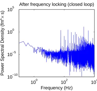
3. The noise in our system is not white. Instead, as shown in the power spectrum resulting from a

measurement of pure buﬀer solution (Figure 3.14), the noise amplitude is signiﬁcantly greater

at frequencies below 10 Hz than it is at frequencies between 10 Hz and 1000 Hz. (Note the spikes

at frequencies greater than 10 Hz represent known narrow-band known noise sources, e.g., 60

Hz electrical noise and its harmonics, which we easily ﬁlter out and do not aﬀect the ultimate

noise level of our measurements.) The higher noise levels below 10 Hz likely stem from physical

eﬀects such as thermal drift, ﬂuid convection, or environmental vibrations. By using a system

that can identify events occurring more rapidly than 10 Hz, the low-frequency noise sources do

not contribute signiﬁcant error to our measurements, whereas they signiﬁcantly impact slower

frequency-swept systems. This reduces the relevant noise ﬂoor in our experiments, enabling

(50)

10

0

10

2

10

4

10

−10

10

−5

10

0

10

5

Frequency (Hz)

Power Spectral Density (fm

2

×

s)

After frequency locking (closed loop)

Figure 3.14: Noise level of system after frequency locking is implemented. The power spectrum of a typical buﬀer data set after the addition of feedback control. The tallest peaks correspond to known noise sources and their multiples.

3.10

Open and Closed Loop Laser Noise Analysis

In this section, we discuss eﬀorts to analyze the noise present from the laser. Note that additional

further post-processing is used to ﬁlter our data and further reduce noise levels.

From speciﬁcations given by the laser manufacturer, Figure 3.15, we estimate our laser frequency

ﬂuctuations to be ∼100 kHz when sampled at a repetition rate of 2 kHz. This corresponds to a noise level of 0.1 femtometers. This number is further reduced by post-processing to remove known

sources of noise and a median ﬁlter. We note that longer PID integration times act as a ﬁlter to

reduce noise, however, if too much of the signal is ﬁltered, then locking cannot occur.

To more precisely analyze the noise present from the laser, one method would be to construct

(51)

ﬂuctu-ations. To reduce intensity noise from the laser, one can monitor the output of the interferometer

using a balanced detector, which subtracts out the noise due to laser intensity ﬂuctuations.

There-fore, the signal from the photodetector will represent the frequency response of our system without

contamination from intensity noise from the laser.

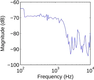
We also provide a Bode plot (Figure 3.16) of our system when the laser is locked to a microtoroid.

This gives the closed loop frequency response of our system. From Figure 3.16, we can see that

our controller responds strongly to laser frequency ﬂuctuations up to repetition rates of ∼ 2 kHz (controller bandwidth), while faster ﬂuctuations cannot be accurately tracked. This shows that our

controller stays locked up to a frequency of 2 kHz.

(52)

10

2

10

3

10

4

−100

−90

−80

−70

−60

Frequency (Hz)

Magnitude (dB)

(53)

Chapter 4

System characterization

4.1

Data processing

4.1.1

Overview

Our data processing occurs in two main steps:

1. ﬁlter the data to reduce noise

2. ﬁnd step (binding) events in our data using a step ﬁnding algorithm

In order to obtain the best approach for our system for our system we compared several methods.

(54)

Remove unwanted frequencies: replace unwanted frequencies with 0 replace unwanted frequencies with nearby surrounding values

mean filter

median filter

total variation denoising

step finding algorithm of Kerssemakers, et al.

generate histogram of binding events Apply non-linear filter:

Find steps:

Process data:

Experimental steps: Specific approaches attempted:

Red box indicates optimal path

Figure 4.1: An overview of our data processing procedure representing all approaches tested. The optimal paths are shown inside the red box.

4.1.2

Filtering

We digitally ﬁlter our data to eliminate known sources of noise. We record the voltage of our

feedback controller outputs at 20,000 Hz using a 24-bit National Instruments data acquisition card

(NI-PCI-4461). The signal that we record is corrupted by the dither signal, which is at a frequency

that we specify and so we may easily ﬁlter out. We accomplish this by taking the Fourier transform

of the data in MATLAB (see Appendix A) and multiplying it with a matrix that is set to 1 for the

values we wish to retain and set to 0 for the values we wish to discard. In this manner, we also ﬁlter

out 60 Hz electronic line noise and all of its subsequent multiples (120, 180, 240, etc.) (Figure 4.2).

We also remove 100 Hz as empirically it was found that the experiments in the lab had 100 Hz noise.

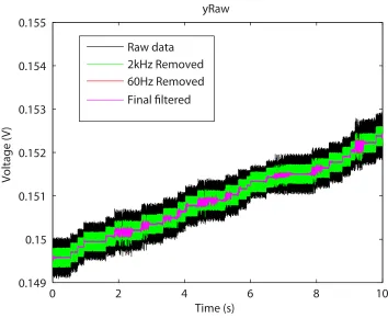
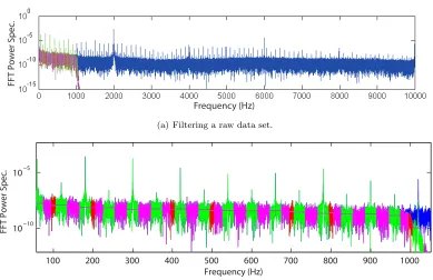
An example of our ﬁltering procedure being performed is shown in Figure 4.3 which represents

data from the selective binding of exosomes (r∼20 nm vesicles) to the microtoroid’s surface. These experiments are discussed in more detail in Section 5.3. We pick exosomes to demonstrate our data

processing technique as they are large biological molecules with clearly observable steps. We show

that the same data processing works for smaller molecules in Section 6. The corresponding time

(55)

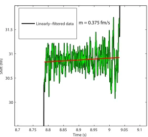
actually have a slight slope (m= 0.38 fm/s) (Figure 4.5(a)) that is the same order of magnitude as

the slope seen in linearly ﬁltered buﬀer data (m = 0.16 fm/s) (Figure 4.5(b)). A slope is present

in the buﬀer (no molecule) data due to index of refraction changes caused by heating due to the

resonant recirculation of light within the microtoroid [67].

raw data

FFT

x

FFT

-1

filtered data

filter

raw freqs

1

0

1

(56)

0

2

4

6

8

10

0.149

0.15

0.151

0.152

0.153

0.154

0.155

yRaw

Time (s)

Voltage (V

)

Raw data

2kHz Removed

60Hz Removed

Final filtered

(57)

Frequency (Hz)

FFT

P

o

w

er Spec

.

(a) Filtering a raw data set.

100 200 300 400 500 600 700 800 900 1000

10−10

10−5

Frequency (Hz)

FFT Power Spec

.

(b) Zoom-in of power spectrum.

(58)

8.7 8.75 8.8 8.85 8.9 8.95 9 9.05 9.1 30

30.5 31 31.5

Time (s)

Shi

ft (fm

)

Linearly−filtered data m = 0.375 fm/s

(a) The plateau region of the particle binding data in Figure 4.3 has a slight slope.

7.5 8 8.5 9 9.5 10

3.5 4 4.5 5 5.5 6 6.5 7

Time (s)

Resonan

ce

w

av

elength shift (fm)

m = 0.164 fm/s

(b) Buﬀer (no molecule) data has a slight slope as well.

(59)

For comparison, we also tried replacing unwanted frequencies with values close to the local

surrounding values as opposed to zero. An example of this ﬁltering method being performed is

shown in Figure 4.4(a). A more clear zoomed in inset of the ﬁlter is shown in Figure 4.4(b).

A comparison between the final filtered data and the filtered data in Figure 4.3 may be seen in

Figure 4.6. As shown in Figure 4.6, replacing unwanted frequencies with zero results in a cleaner

(60)

0.5 0.6 0.7 0.8 0.9 1 0.1493

0.1494 0.1495 0.1496 0.1497 0.1498 0.1499 0.15 0.1501 0.1502

yRaw

Time (s)

Voltage (V

)

0.5 0.6 0.7 0.8 0.9 1 0.1493

0.1494 0.1495 0.1496 0.1497 0.1498 0.1499 0.15 0.1501 0.1502

yRaw

Time (s)

Voltage (V)

a

b

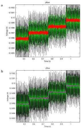
Figure 4.6: Zoomed in comparison between replacing unwanted frequencies with nearby frequencies (a) and replacing unwanted frequencies with zero (b). The green trace shows the data after the 2 kHz dither signal has been removed. Red represents the data after 60 Hz electronic line noise and its multiples has been removed, and magenta shows the ﬁnal ﬁltered data. Replacing unwanted frequencies with 0 results in better a signal-to-noise ratio.

4.1.3

Median ﬁltering

After removing unwanted frequencies, we can further improve the signal-to-noise ratio by applying a

(61)

of the window. This method is often preferred over the moving average as the moving average may

smooth out desired steps. To determine the optimal window size for our data, we experimented with

several diﬀerent window sizes. Figure 4.7 shows the data after applying the zero ﬁlter with median

ﬁlters of varying window sizes applied. From Figure 4.7 we conclude that a window size of 1001

points (total data length is 200,000 points or 10 seconds) is optimal.

0 2 4 6 8 10

−50 −40 −30 −20 −10 0 10 20 30 40 50

y With Median Filters

Time (s)

Shift (fm

)

Linearly−filtered data Median Window 5 Median Window 11 Median Window 101 Median Window 1001

(a) Median ﬁlters of varying window sizes being applied to the data.

5.4 5.6 5.8 6 6.2 6.4 6.6

0 5 10 15 20 25

y With Median Filters

Time (s)

Shift (fm

)

Linearly−filtered data Median Window 5 Median Window 11 Median Window 101 Median Window 1001

(b) A zoom in of median ﬁlters of diﬀerent window sizes being applied

(62)

Figure 4.8 shows an overlay of the linearly ﬁltered data before and after the median ﬁlter with

a window size of 1001 has been performed.

0 1 2 3 4 5 6 7 8 9 10

−50 −40 −30 −20 −10 0 10 20 30 40 50

Linear filtered data (black) and Median filtered data with window size 1001 (red)

Time (s)

Shift (fm)

Figure 4.8: A time trace of the data after a median ﬁlter of 1001 points has been performed (red).

4.1.4

Total variation denoising

We also examined the eﬀects of applying a noise removal technique known as total variation denoising

(TVD) to our data. TVD is a signal processing technique developed by Rudin in 1992 [68] that

has been shown to reduce noise while preserving sharp edges. The algorithm works by ﬁnding an

approximate signal that is close to the original signal but with less variation (noise). TVD has been

reported to be better at detecting step like events than either a mean or median ﬁlter [69].

In more detail, the algorithm minimizes the sum of two terms: (1) a measure of how close the

approximate signal is to the original signal and (2) an expression for the variation. The variation

V(y) of a signal may be deﬁned as:

V(y) =∑

n

(63)

One measure of how close an approximate signal (yn) is with the data trace (xn) is the sum of square

errors between the two:

E(x, y) =1

2

∑

n

(xn−yn)2 (4.2)

The sum of these two may be written as:

E(x, y) +λV(y) (4.3)

where λ is a user-defined parameter known as the regularization parameter that affects that amount of denoising that occurs. Ifλis too small, no denoising will occur, however, ifλis too large, a flat line will result (i.e., variation will be minimized, but the approximation signal will look nothing

like the input signal). The goal of TVD is to ﬁnd aynsuch that Equation 4.3 is minimized. For our

work we use code provided by Max Little [69]. Fig