R E S E A R C H
Open Access
A fourth order accurate approximation of the
first and pure second derivatives of the
Laplace equation on a rectangle
Adiguzel A Dosiyev
*and Hamid MM Sadeghi
*Correspondence:
[email protected] Department of Mathematics, Eastern Mediterranean University, Famagusta, KKTC, Mersin 10, Turkey
Abstract
In this paper, we discuss an approximation of the first and pure second order derivatives for the solution of the Dirichlet problem on a rectangular domain. The boundary values on the sides of the rectangle are supposed to have the sixth derivatives satisfying the Hölder condition. On the vertices, besides the continuity condition, the compatibility conditions, which result from the Laplace equation for the second and fourth derivatives of the boundary values, given on the adjacent sides, are also satisfied. Under these conditions a uniform approximation of order
O(h4) (his the grid size) is obtained for the solution of the Dirichlet problem on a square grid, its first and pure second derivatives, by a simple difference scheme. Numerical experiments are illustrated to support the analysis made.
Keywords: finite difference method; approximation of derivatives; uniform error; Laplace equation
1 Introduction
Since the operation of differentiation is ill conditioned, to find a highly accurate approxi-mation for the derivatives of the solution of a differential equation becomes problematic, especially when the smoothness is restricted.
In [], it was proved that the higher order difference derivatives uniformly converge to the corresponding derivatives of the solution of the Laplace equation in any strictly interior subdomain, with the same order ofhas which the difference solution converges on the given domain. In [], by using the difference solution of the Dirichlet problem for the Laplace equation on a rectangle, the uniform convergence of its first and pure second divided difference over the whole grid domain to the corresponding derivatives of the exact solution with the rateO(h) is proved. In [], the difference schemes on a rectangular
parallelepiped were constructed, where solutions approximate the Dirichlet problem for the Laplace equation and its first and second derivatives. Under the assumptions that the boundary functions belong toC,λ, <λ< , on the faces, are continuous on the edges, and their second-order derivatives satisfy the compatibility condition, the solution to their difference schemes converges uniformly on the grid with the rate ofO(h).
In this paper, we consider the Dirichlet problem for the Laplace equation on a rectangle, when the boundary values belong toC,λ, <λ< , on the sides of the rectangle and as a whole are continuous on the vertices. Also the τ,τ= , , order derivatives satisfy the
compatibility conditions on the vertices which result from the Laplace equation. Under these conditions, we construct the difference problems, the solutions of which converge to the first and pure second derivatives of the exact solution with the orderO(h). Finally,
numerical experiments are given in the last part of the paper to support the theoretical results.
2 The Dirichlet problem on rectangular domains
Let={(x,y) : <x<a, <y<b}be a rectangle,a/bbe rational,γj(γj),j= , , , , be the
sides, including (excluding) the ends, enumerated counterclockwise starting from the left side (γ≡γ,γ≡γ), and letγ =
j=γjbe the boundary of. Denote bysthe arclength,
measured alongγ, and bysjthe value ofsat the beginning ofγj. We say thatf∈Ck,λ(D),
iff haskth derivatives onDsatisfying a Hölder condition with exponentλ∈(, ). We consider the boundary value problem
u= on, u=ϕj(s) onγj,j= , , , , ()
where≡∂/∂x+∂/∂y,ϕ
jare given functions ofs. Assume that
ϕj∈C,λ(γj), <λ< ,j= , , , , ()
ϕj(q)(sj) = (–)qϕj(–q)(sj), q= , , . () Lemma . The solution u of problem()is from C,λ().
The proof of Lemma . follows from Theorem . in [].
Lemma . The inequality is true
max
≤p≤(xsup,y)∈
∂u
∂xp∂y–p
<∞, ()
where u is the solution of problem().
Proof From Lemma . it follows that the functions ∂∂xu and ∂u
∂y are continuous on. We putw=∂∂xu. The functionwis harmonic inand is the solution of the problem
w= on, w= j onγj,j= , , , ,
where
τ= ∂ϕτ
∂y , τ= , ,
ν=∂
ϕν
∂x , ν= , .
From the conditions () and () it follows that
Hence, on the basis of Theorem . in [], we have
Similarly, it is proved that
sup
From ()-(), estimation () follows.
Lemma . Letρ(x,y)be the distance from a current point of the open rectangleto its
where c is a constant independent of the direction of the derivative∂/∂l,u is a solution of problem().
Proof According to Lemma ., we have
max
Since any eighth order derivative can be obtained by two times differentiating some of the derivatives∂/∂xp∂y–p, ≤p≤, on the basis of estimations () and () from [],
From (), inequality () follows.
Leth> , anda/h≥,b/h≥ be integers. We assignh, a square net on, with steph,
Let the operatorBbe defined as follows:
Bu(x,y) =u(x+h,y) +u(x–h,y) +u(x,y+h) +u(x,y–h)/
+u(x+h,y+h) +u(x+h,y–h)
We consider the classical -point finite difference approximation of problem ():
uh=Buh onh, uh=ϕj onγjh∪ ˙γj,j= , , , . ()
By the maximum principle, problem () has a unique solution.
In what follows, and for simplicity, we will denote by c,c,c, . . . constants which are
independent ofhand the nearest factor, and identical notation will be used for various constants.
Lethbe the set of nodes of the gridhthat are at a distancehfromγ, and leth= h\h.
Lemma . The following inequality holds:
max
(x,y)∈(h∪h)|Bu–u| ≤ch
, ()
where u is a solution of problem().
Proof Let (x,y) be a point ofh, and let
R= (x,y) :|x–x|<h,|y–y|<h
()
be an elementary square, some sides of which lie on the boundary of the rectangle. On the vertices ofRand on the mid-points of its sides lie the nodes of which the function
values are used to evaluateBu(x,y).
We represent a solution of problem () in some neighborhood of (x,y)∈h by
Tay-lor’s formula
u(x,y) =p(x,y) +r(x,y), ()
wherep(x,y) is the seventh order Taylor’s polynomial,r(x,y) is the remainder term.
Tak-ing into account that the functionuis harmonic, by exhaustive calculations, we have
Bp(x,y) =u(x,y). ()
Now, we estimaterat the nodes of the operatorB. We take a node (x+h,y+h) which
is one of the eight nodes ofB, and we consider the function
u(s) =u
x+
s
√ ,y+
s
√
, –√h≤s≤√h ()
of one variables. By virtue of Lemma ., we have
ddsu(s)
≤c(√h–s)–, ≤s<√h. ()
We represent function () around the points= by Taylor’s formula
wherep(s)≡p(x+√s,y+√s) is the seventh order Taylor’s polynomial of the variables,
and
r(s)≡r
x+
s
√ ,y+
s
√
, ≤ |s|<√h, ()
is the remainder term.
On the basis of () and the integral form of the remainder term of Taylor’s formula, we have
r(
√
h–ε)≤c !
√
h–ε
(√h–ε–t)(√h–t)–dt≤ch, <ε≤
h
√
. ()
Taking into account the continuity of the functionr(s) on [–
√
h,√h], from () and (), we obtain
r(x+h,y+h)≤ch, ()
wherecis a constant independent of the point taken, (x,y) onh.
Estimation () is obtained analogously for the remaining seven nodes of the operatorB. Since the norm of the operator is equal to in the uniform metric, by using (), we have
Br(x,y)≤ch. ()
Hence, on the basis of (), (), (), and linearity of the operatorB, we obtain
Bu(x,y) –u(x,y)≤ch,
for any (x,y)∈h.
Now, let (x,y) be a point ofh, and let in the Taylor formula () corresponding to this
point, the remainder termr(x,y) be represented in the Lagrange form. ThenBr(x,y)
contains eighth order derivatives of the solution of problem () at some points of the open squareRdefined by (), when (x,y)∈h. The squareRlies at a distance from the
boundaryγ of the rectangle; it is not less thanh. Therefore, on the basis of Lemma ., we obtain
Br(x,y)≤ch, ()
wherecis a constant independent of the point (x,y)∈h. Again, on the basis of (),
(), and () follows estimation () at any point (x,y)∈h. Lemma . is proved.
We present two more lemmas. Consider the following systems:
qh=Bqh+gh onh, qh= onγh, ()
qh=Bqh+gh onh, qh≥ onγh, ()
Lemma . The solutions qhand qhof systems()and()satisfy the inequality
|qh| ≤qh on h
.
The proof of Lemma . follows from the comparison theorem (see Chapter in []).
Lemma . For the solution of the problem
qh=Bqh+h onh, qh= onγh, ()
the following inequality holds:
qh≤
ρdh
onh,
where d=max{a,b},ρ=ρ(x,y)is the distance from the current point(x,y)∈h to the boundary of the rectangle.
Proof We consider the functions
q()h (x,y) = h
ax–x≥, q()
h (x,y) =
h
by–y≥ on,
which are solutions of the equationqh=Bqh+honh. By virtue of Lemma ., we obtain
qh≤min i=,q
(i)
h (x,y)≤
ρdh
onh.
Theorem . Assume that the boundary functionsϕj,j= , , , satisfy conditions()
and().Then
max
h
|uh–u| ≤cρh, ()
where uhis the solution of the finite difference problem(),and u is the exact solution of
problem().
Proof Let
εh=uh–u on h
. ()
It is obvious that
εh=Bεh+ (Bu–u) onh, εh= onγh. ()
By virtue of estimation () for (Bu–u) and by applying Lemma . to the problems () and (), on the basis of Lemma . we obtain
max
h
|εh| ≤cρh. ()
3 Approximation of the first derivative
We denotej=∂∂ux onγj,j= , , , , and consider the boundary value problem:
v= on, v=j onγj,j= , , , , ()
whereuis a solution of the boundary value problem (). We put
whereuhis the solution of the finite difference boundary value problem ().
Lemma . The following inequality is true:
kh(uh) –kh(u)≤ch, k= , , ()
where uhis the solution of problem(),u is the solution of problem().
Proof On the basis of (), (), and Theorem ., we have
Lemma . The following inequality holds
max the fourth order approximation of ∂∂ux, respectively. From the truncation error formulas (see []) it follows that
max
On the basis of Lemma . and estimation () follows (). We consider the finite difference boundary value problem
vh=Bvh onh, vh=jh onγjh,j= , , , , ()
Theorem . The estimation is true
max
(x,y)∈h
vh–
∂u ∂x
≤ch, ()
where u is the solution of problem(),vhis the solution of the finite difference problem().
Proof Let
h=vh–v on h
, ()
wherev=∂u
∂x. From () and (), we have
h=Bh+ (Bv–v) onh, h=kh(uh) –v onγkh,k= , ,
h= onγph,p= , .
()
We represent
h=h+h, ()
where
h=Bh onh, ()
h=kh(uh) –v onγkh,k= , , h= onγph,p= , , ()
h=Bh+ (Bv–v) onh, h= onγjh,j= , , , . ()
By Lemma . and by the maximum principle, for the solution of system (), (), we have
max
(x,y)∈h
h≤max q=,(xmax,y)∈γh
q
qh(uh) –v≤ch. ()
The solutionhof system () is the error of the approximate solution obtained by the finite difference method for problem (), when the boundary values satisfy the conditions
j∈C,λ(γj), <λ< ,j= , , , , ()
j(q)(sj) = (–)qj(–q)(sj), q= , . ()
Since the functionv=∂∂ux is harmonic onwith the boundary functionsj,j= , , , ,
on the basis of (), (), and Remark in [], we have
max
(x,y)∈h
h≤ch. ()
4 Approximation of the pure second derivatives
We denoteω=∂∂xu. The functionωis harmonic on, on the basis of Lemma . is con-tinuous onand is a solution of the following Dirichlet problem:
ω= on, ω=j onγj,j= , , , , ()
where
τ= ∂ϕ
τ
∂x , τ= , , ()
ν= – ∂ϕν
∂y , ν= , . ()
From the continuity of the functionωonand from (), () and (), () it follows that
j∈C,λ(γj), <λ< ,j= , , , , () (q)
j (sj) = (–)qj(–q)(sj), q= , ,j= , , , . ()
Letωhbe a solution of the finite difference problem
ωh=Bωh onh, ωh=j onγjh∪ ˙γj,j= , , , , ()
wherej,j= , , , , are the functions determined by () and ().
Theorem . The following estimation holds:
max
h
|ωh–ω| ≤ch, ()
whereω=∂u
∂x,u is the solution of problem()andωhis the solution of the finite difference
problem().
Proof On the basis of conditions () and (), the exact solution of problem () belongs to the class of functionsC,λ() (see []). Therefore, inequality () follows from the re-sults in [] (see Remark ), as the case of the Dirichlet problem.
5 Numerical example
Let={(x,y) : – <x< , <y< }, and letγ be the boundary of . We consider the following problem:
u= on, u=p(x,y) onγj,j= , , , , ()
where
p(x,y) =x+ycos
arctan
y x
()
Let U be the exact solution and Uh be its approximate values on h
of the Dirich-let problem on the rectangular domain . We denote U–Uhh =max
h|U–Uh|, m
U=
U–U–mh U–U–(m+)
h
.
In Table and in Table , the maximum errors and the convergence order of the approx-imations of the first and pure second derivatives of problem () for different step sizesh are presented.
The results show that the approximate solutions converge asO(h).
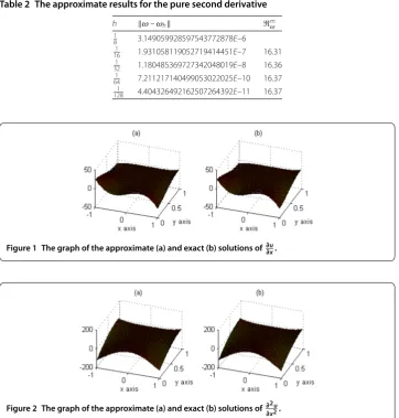
The shapes of ∂∂ux and ∂∂xu and their approximations are demonstrated in Figure and Figure , respectively.
Table 1 The approximate results for the first derivative
h v–vh mv
1
8 2.299996064764325009657E–2 1
16 1.894059104568160525104E–3 12.14 1
32 1.344880793701474553783E–4 14.08 1
64 8.960663249977644986927E–6 15.01 1
128 5.796393863873542692774E–7 15.46
Table 2 The approximate results for the pure second derivative
h ω–ωh mω
1
8 3.149059928597543772878E–6 1
16 1.931058119052719414451E–7 16.31 1
32 1.180485369727342048019E–8 16.36 1
64 7.211217140499053022025E–10 16.37 1
128 4.404326492162507264392E–11 16.37
Figure 1 The graph of the approximate (a) and exact (b) solutions of∂u∂x.
Figure 2 The graph of the approximate (a) and exact (b) solutions of∂2u
6 Conclusion
The obtained results can be used to highly approximate the derivatives for the solution of Laplace’s equation by the finite difference method, in some version of domain decom-position methods, in composite grid methods, and in the combined methods for solving Laplace’s boundary value problems on polygons (see [–]).
Competing interests
The authors declare that they have no competing interests.
Authors’ contributions
All authors contributed equally to the writing of this paper. All authors read and approved the final manuscript.
Received: 4 November 2014 Accepted: 9 February 2015
References
1. Lebedev, VI: Evaluation of the error involved in the grid method for Newmann’s two dimensional problem. Sov. Math. Dokl.1, 703-705 (1960)
2. Volkov, EA: On convergence inc2of a difference solution of the Laplace equation on a rectangle. Russ. J. Numer. Anal. Math. Model.14(3), 291-298 (1999)
3. Volkov, EA: On the grid method for approximating the derivatives of the solution of the Dirichlet problem for the Laplace equation on the rectangular parallelpiped. Russ. J. Numer. Anal. Math. Model.19(3), 269-278 (2004) 4. Volkov, EA: Differentiability properties of solutions of boundary value problems for the Laplace and Poisson
equations on a rectangle. Proc. Steklov Inst. Math.77, 101-126 (1965)
5. Volkov, EA: On differential properties of solutions of the Laplace and Poisson equations on a parallelepiped and efficient error estimates of the method of nets. Proc. Steklov Inst. Math.105, 54-78 (1969)
6. Volkov, EA: On the solution by the grid method of the inner Dirichlet problem for the Laplace equation. Transl. Am. Math. Soc.24, 279-307 (1963)
7. Samarskii, AA: The Theory of Difference Schemes. Marcel Dekker, New York (2001) 8. Burden, RL, Faires, JD: Numerical Analysis. Brooks/Cole, Cengage Learning, Boston (2011)
9. Dosiyev, AA: On the maximum error in the solution of Laplace equation by finite difference method. Int. J. Pure Appl. Math.7(2), 229-241 (2003)
10. Dosiyev, AA: The high accurate block-grid method for solving Laplace’s boundary value problem with singularities. SIAM J. Numer. Anal.42(1), 153-178 (2004)
11. Volkov, EA, Dosiyev, AA: A high accurate composite grid method for solving Laplace’s boundary value problems with singularities. Russ. J. Numer. Anal. Math. Model.22(3), 291-307 (2007)
12. Dosiyev, AA: The block-grid method for the approximation of the pure second order derivatives for the solution of Laplace’s equation on a staircase polygon. J. Comput. Appl. Math.259, 14-23 (2014)