A graph theoretic approach to global input to state stability for coupled control systems

(1)

R E S E A R C H

Open Access

A graph-theoretic approach to global

input-to-state stability for coupled

control systems

Yu Qiao

1*

_{, Yue Huang}

2

_{and Minghao Chen}

3

*_{Correspondence:} [email protected] 1_{School of Mathematics and} Statistics, Shandong University, Weihai, Weihai, 264209, P.R. China Full list of author information is available at the end of the article

Abstract

In this paper, the input-to-state stability for coupled control systems is investigated. A systematic method of constructing a global Lyapunov function for the coupled control systems is provided by combining graph theory and the Lyapunov method. Consequently, some novel global input-to-state stability principles are given. As an application to this result, a coupled Lurie system is also discussed. By constructing an appropriate Lyapunov function, a suﬃcient condition ensuring input-to-state stability of this coupled Lurie system is established. Two examples are provided to

demonstrate the eﬀectiveness of the theoretical results.

Keywords: input-to-state stability; coupled control system; Lyapunov function

1 Introduction

In recent years, coupled control systems (CCSs) have received considerable attention for their interesting characteristics from the mathematical point of view. The main interest has been focused on the investigation of the global dynamics of the systems, with a spe-cial emphasis on the study of stability. Meanwhile, input-to-state stability (ISS) for control systems has been extensively studied due to a wide range of applications in physics, biol-ogy, social science, neural networks, engineering fields, and artificial complex dynamical systems. For example, Sontag and Wang [] showed the importance of the well-known Lyapunov sufficient condition for ISS and provided additional characterizations of the ISS property, including one in terms of nonlinear stability margins. Grüne [] presented a new variant of the ISS property which is based on a one-dimensional dynamical system, showed the relation to the original ISS formulation, and described the characterizations by means of suitable Lyapunov functions. In [], Angeli presented a framework for under-standing such questions fully compatible with the well-known ISS approach and discussed applications of the newly introduced stability notions. In [], Arcak and Teel analyzed ISS for the feedback interconnection of a linear block and a nonlinear element.

As far as we know, there are a lot of papers dealing with the ISS of individual control systems but few papers dealing with the ISS of CCSs. In general, the study of ISS for CCSs is complex, because it is very diﬃcult to straightly construct an appropriate Lyapunov function for CCSs. However, in [], Li and Shuai studied the global-stability problem of

(2)

equilibrium and developed a systematic approach that allows one to construct global Lya-punov functions for large-scale coupled systems from building blocks of individual vertex systems. Later, this technique was appropriately developed and extended to some other coupled systems. In [–] several delayed coupled systems were discussed, and some suf-ﬁcient conditions were obtained. Li et al. in [–] investigated the stochastic stability of coupled systems with both white noise and color noise. Moreover, by using this technique, Su et al. derived suﬃcient conditions ensuring global stability of discrete-time coupled sys-tems [, ], and Zhang et al. extended this technique to multi-dispersal coupled syssys-tems []. Besides, this technique is also applied to many practical applications, such as biolog-ical systems [–], neural networks [, ], and mechanbiolog-ical systems [–]. Hence, the graph theory is a great method in the study of coupled systems.

Motivated by the above discussions, in this paper, we investigate the ISS of CCSs. A sys-tematic method of constructing a global Lyapunov function for the CCSs is provided by combining graph theory and the Lyapunov method. Consequently, some novel global sta-bility principles are given. As an application to this result, a coupled Lurie system is also discussed. By constructing an appropriate Lyapunov function, a suﬃcient condition en-suring the ISS of this coupled Lurie system is established. Finally, two examples and their numerical simulations are provided to demonstrate the eﬀectiveness and correctness of the theoretical results.

The rest of the paper is organized as follows. In Section , some preliminaries and the problem description are presented. In Section , the main theorems and their rigorous proofs are described. Finally, in Section , an application to a coupled Lurie system is given, and the respective simulations are also given to demonstrate the eﬀectiveness of our results.

2 Preliminaries and model formulation

Throughout the paper, unless otherwise speciﬁed, the following notations will be used. As we usually use,Rndenotes then-dimensional Euclidean space. NotationsR₊= [, +∞),

Z+₌_{_{, , . . .}_}_,_L₌_{_{, , . . . ,}_l}_,_n₌l

i=ni, andm= l

i=miforni,mi∈Z+are used. For

anyx∈Rn_,_xT_{is its transpose and}_|_x_|_{is its Euclidean norm. Let}_Rn×n_{denote the set of} n×nreal matrix space. For a matrixP,P≥ (≤) means thatPis positive semi-deﬁnite (negative semi-deﬁnite). The symbolψ◦ψstands for the composition of two functions

ψandψ. The gradient function of a functionf is indicated byf. In anm-dimensional

space, the symbolLm

∞indicates the set of all the functions which are endowed with

essen-tial supremum normu=sup{|u(t)| |t≥} ≤ ∞.

We recall some knowledge of graph theory that will be used in the rest of the paper. Deﬁne a weighted digraphG={V,E,A}, in which setV={v,v, . . . ,vl}denoteslvertices

of the graph, elementeijofEdenotes the arc leading from initial vertexjto terminal vertex i, and the elementaijof a weighted adjacency matrixAdenotes the weight of arceij. We

denoteaij>  if and only if there exists an arc from vertexito vertexjinG, otherwiseaij=

, and we denoteaii=  for alli∈L. Denote the digraph with weight matrixAas (G,A). If a

graphShas the same vertex asG, we call it a subgraph ofG. The weightW(S) of a subgraph

S is the product of the weights on all its arcs. If a connected subgraph has no cycle, it is a tree. We callvithe root of the tree if vertexiof the tree is not a terminal vertex of any

(3)

Laplacian matrix ofGis deﬁned asL= (bij)l×l, wherebij= –aijfori=jandbij=

k=iaik

fori=j.

The following lemma will be used in the proof of our main results.

Lemma ([]) Assume l≥.Then the following identity holds:

l

i,j=

ciaijFij(xi,xj) =

Q∈Q

W(Q)

(s,r)∈E(C_Q)

Frs(xr,xs).

Here Fij(xi,xj)are arbitrary functions for any≤i,j≤l,aijare elements of matrix A,Qis the set of all spanning unicyclic graphs of(G,A),W(Q)is the weight ofQ,and C_Qdenotes the directed cycle ofQ.And ci denotes the cofactor of the ith diagonal element of L, in particular,if(G,A)is strongly connected,then ci> for≤i≤l.

In the remainder of this section, we shall give the model formulation and state some deﬁnitions that will be used in the main results.

Given a digraph (G,A) withlvertices (l≥) andA= (aij)l×l. A coupled control system

can be constructed on (G,A) by assigning each vertex its own dynamics and then coupling these vertex dynamics based on directed arcs in (G,A). The details are as follows. Assume that theith vertex dynamic is described by the control system

˙ xi(t) =fi

xi(t),ui

, t≥,

wherexi∈Rnidenotes the value of vertexi,fi:Rni×Rmi→Rniis continuously

diﬀeren-tiable and satisﬁesfi(, ) = , functionui:R+→Rmidenotes the input of vertexiand it

is measurable and locally essentially bounded. Assume thataij≥ represents the eﬀect

factor from vertexjto vertexiandaij=  iﬀ there exists no arc fromjtoi. Then we use

functionPijto describe the eﬀect that subsystemjhas oniandPij:Rni×Rnj×Rmj→Rni

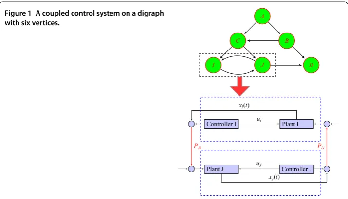
is continuously diﬀerentiable and satisﬁesPij(, , ) = . For example, in a digraph with

six vertices, we show the interaction in vertexjand vertexi(see Figure ).

(4)

Then coupling the vertex systems together, we obtain the following coupled control

sys-To be more precise, we recall some deﬁnitions on the ISS of CCS (). We refer to [, ] for deﬁnitions as follows.

Deﬁnition  A functionγ :R

In the proof of our main results, we need to ﬁnd a global ISS-Lyapunov function for CCS (). For the convenience of the proof, we now deﬁne vertex ISS-Lyapunov functions for CCS ().

Deﬁnition  Set{Vi(xi),i∈L}is called a vertex ISS-Lyapunov function set for CCS () if

everyVi(xi) is smooth and satisﬁes the following conditions:

(5)

3 Main results

In this section, the ISS of CCS () will be investigated. The approaches used in the proof of the main results are motivated by [, ].

Theorem  If CCS()admits a vertex ISS-Lyapunov function set{Vi(xi),i∈L},and

di-in whichciis the cofactor of theith diagonal element of Laplacian matrix of (G,D).

(6)

This implies that

in whichδ>  is a certain constant. For simplicity, we write

(7)

Since the digraph is strongly connected, it implies thatci> , and thenα> ,δ> . Thus

sequently, from condition Q, we can derive

˙

we can obtain from condition Q that

V(x) =

In [], the ISS for individual nonlinear control system was investigated by Sontag and Wang. Some classes of stability, like robust stability and weak robust stability for control systems, were investigated and some suﬃcient conditions were established to guarantee these stabilities. Motivated by [], we have the following results.

Theorem  Let the conditions in Theoremhold.Then: () CCS()is robustly stable.

(8)

() For eachε> ,there existsδ> such that|x(t,x,u)| ≤εfor all inputsu∈Lm∞and initial statesxwith|x| ≤δandu ≤δ.

() There exists aK-functionγ such that,for anyr,ε> ,there isT> so that for every inputu∈Lm_∞,it holds that|x(t,x,u)| ≤ε+γ(u),whenever|x| ≤randt≥T.

() CCS()is weakly robustly stable.

4 An application to a coupled Lurie system

Now in order to illustrate the result of Theorem , let us apply this result to a coupled Lurie system (CLS). The absolute stability problem, formulated by Lurie and coworkers in the s, has been a well-studied and fruitful area of research.

Assume that each vertex dynamic is described by a feedback interconnection of a linear block and a nonlinear element. To be simpliﬁed,xi(t) andyi(t) are denoted byxiandyi, i= , , . . . ,l. When a bounded input is set to every vertex system, it can be described as

˙

xi=Aixi+Bi

–αi(yi) +ui

,

yi=Kixi,

wherexi∈Rni,yi∈Rmi,Ki∈Rmi×ni,Ai∈Rni×niis the personal state alteration matrix for

theith vertex system,Bi∈Rni×miis the feedback and input eﬀect matrix,uidenotes the

input of vertexi, andαi(·) :Rmi→Rmiis a feedback function. LetDj∈Rni×njdescribe the

eﬀect that vertex systemjhas oni. Thus a CLS is obtained as follows:

˙

xi=Aixi+Bi

–αi(yi) +ui

+

l

j=

Djxj,

yi=Kixi.

()

Before the main theorem, let us present some assumptions and two lemmas. The fol-lowing fundamental assumptions for CLS () are given:

A: If(Ai,Ki)is detectable and there exists matrixPi=PTi ≥satisfying AT_iPi+PiAi+l

PT_iPi+DTiDi

≤, K_iT=PiBi. ()

A: Ifϕiis aK∞-function, and for allyi∈Rmi,

|yi|ϕi

|yi|

≤yT_iαi(yi). ()

A: When|yi| ≥μi, whereμi> 

αi(yi)≤yTiαi(yi). ()

The results in this section and their proofs are motivated by [].

Lemma  For CLS(),there exist a constantθi> and aK∞-functionηi(·)satisfying

θiαi(yi)+|yi|

(9)

when|yi| ≥μi,

ηi

|yi|

|yi|+ηiαi(yi)αi(yi)



≤yT_iαi(yi) ()

when|yi| ≤μi.

The proof of Lemma  can be seen in [].

Since it is complex to construct a vertex ISS-Lyapunov function for CLS (), we ﬁrstly construct a section of the vertex ISS-Lyapunov function in the following lemma. And then we give the entire vertex ISS-Lyapunov function for CLS () in the main theorem.

Lemma  Suppose that()satisﬁes assumptionsA-A.Deﬁnite a function

σi(r) =εi r



min

,√

z,πi(z)

dz,

where the constantεi> and theK-functionπi(·)is to be speciﬁed.Let Si(xi) =σi(xTiQixi), in which matrix QT

i =Qi> satisfying

(Ai–JiKi)TQi+Qi(Ai–JiKi) +l

QT_iQi+DTiDi

≤–I, ()

then there exists aK-functionγi(·)satisfying

˙

Si(xi)≤–γi

|xi|

+yT_iαi(yi) +θi|ui|+ l

j=

Fij(xi,xj),

where Fij(xi,xj) =xTjDTjDjxj–xTiDTiDixi. Proof Rewrite CLS () as

˙

xi= (Ai–JiKi)xi+Jiyi+Bi

–αi(yi) +ui

+

l

j=

Djxj, ()

whereJiis chosen so thatAi–JiKiis a Hurwitz matrix. By the construction ofSi(·), it is

easy to see thatSi(·) is positive deﬁnite and radially unbounded. Then we letk>  satisfy

maxBT_iQixi,JiTQixi≤k|xi|

for all ≤i≤l, and note from () that

˙

Si(xi)≤σi

xT_iQixi

xT_iQi (Ai–JiKi)xi+ l

j=

Djxj

+k|xi|αi(yi)+|yi|+|ui|

. ()

Becauseσ_i(z)≤εi/√z, we can ﬁnd a constantci> , independent ofεi, so thatσi(xTiQixi)× k|xi| ≤ciεifor allxi∈Rni. And then we can obtain

˙

Si(xi)≤σi

xT_iQixi

xT_iQi (Ai–JiKi)xi+ l

j=

Djxj

+ciεiαi(yi)+|yi|+|ui|

(10)

(11)

then substituting () and () into () yields

The proof is complete.

(12)

=lPT_iPi+DTjDj

|xi|+ l

j=

DT_jDj|xj|–DTiDi|xi|

=lxT_iPT_iPixi+xTiDTiDixi

+

l

j=

Fij(xi,xj).

Noting thatAT_iPi+PiAi+l(PTiPi+DTiDi)≤, we get

˙

Ri(xi)≤–yTiαi

yi+ yTiui

+

l

j=

Fij(xi,xj).

Considering the two cases|ui| ≤ϕi(|yi|)/ and|ui| ≥ϕi(|yi|)/ and using (), we obtain the

inequality

yT_iui≤|yi||ui| ≤ |yi|ϕi

|yi|+ (ϕi)–

|ui|

|ui| ≤yTiαi(yi) + (ϕi)–

|ui|

|ui|,

which results in

˙

Ri(xi)≤–yiTαi(yi) + ϕi–

|ui|

|ui|+ l

j=

Fij(xi,xj).

From Lemma , we knowS˙i(xi)≤–γi(|xi|) +yTiαi(yi) +θi|ui|+ l

j=Fij(xi,xj). Then we have

Li(xi)≤–γi

|xi|

+βi

|ui|

+

l

j=

Fij(xi,xj)

withβi(|ui|) =δi|ui|+ φi–(|ui|)|ui|. Then we can ﬁndξi>  satisfying

˙

Li(xi)≤–ξi|xi|p+ l

j=

Fij(xi,xj).

So we conclude thatLi(xi) is a vertex ISS-Lyapunov function, then from Theorem , CLS

() is ISS.

Remark  In recent years, Lurie systems have been studied by many researchers [, ]. Particularly, compared with [], the main diﬀerences are as follows.

(i) This paper considers a coupled Lurie system, which is more complicated. (ii) This paper uses graph theory combining with the Lyapunov method to derive the

ISS of the considered system. This technique does not need us solving any linear matrix inequality. Literature [] proposed Lyapunov-Krasovskii functionals which contain an exponential multiplier to solve the stabilization of an indirect control system.

(iii) In [], time delay was considered, which is our further work.

(13)

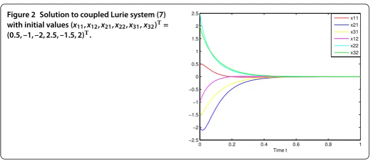
Figure 2 Solution to coupled Lurie system (7) with initial values (x11,x12,x21,x22,x31,x32)T= (0.5, –1, –2, 2.5, –1.5, 2)T_.

Example  Assume that there are three vertices andxi= (xi,xi)T∈R. We now take the

following coeﬃcients for (), and then take some numerical simulation. Here,

Ai=

– 

 –

, Bi=

 

,

D=

 

 

, D=

 

, D=

 

 

.

And let the input functionui= ,αi(yi) =iyi,i= , , . Moreover, we takeϕi(yi) =_iyiand μi=  fori= , , . It is clear that conditions A and A are satisﬁed. If we let

P=

 

 

, P=

 

 

, P=

 

 

,

by calculation, we get that condition A holds. Therefore, by Theorem , we derive that () is ISS. The respective simulation results are shown in Figure , which conforms the eﬀectiveness of the developed results.

Example  We consider the ISS of a system described as follows:

˙

xi=Aixi+Biyi+



j=

Djxj,

˙

yi= –Kixi– yi–φi(yi) –ui+



j=

yj,

i= , , , ()

with the input functionui=Ci(xTi,yi)Tin whichCiis a matrix andxi= (xi,xi)T, function

φi(yi) =yi, and there exist matricesPTi =Pi≥ such that

AT_iPi+PiAi+ 

P_iTPi+DTiDi

≤,

K_iT=PiBi,

(14)

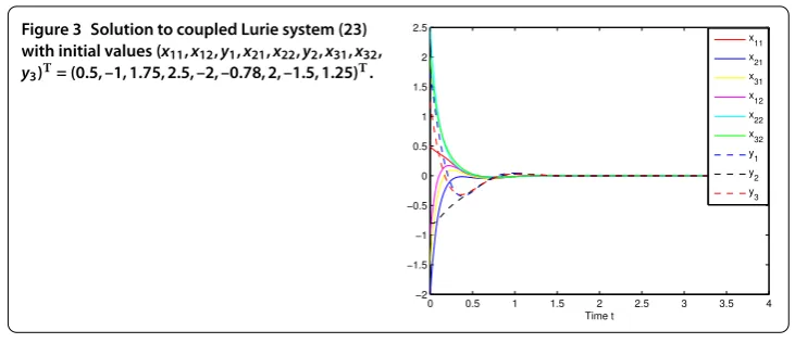
Figure 3 Solution to coupled Lurie system (23) with initial values (x11,x12,y1,x21,x22,y2,x31,x32, y3)T= (0.5, –1, 1.75, 2.5, –2, –0.78, 2, –1.5, 1.25)T.

To apply Theorem , we rewrite () as in (), with

Ai=

Ai Bi

–Ki –

, Bi=

 

, Pi= Pi 

 

, Di= Di 

 

andαi(yi) = yi+φi(yi). Thenαi(yi) satisﬁes conditions A and A. And then, we let the

values ofAi,Bi,Di,Pi,i= , , , be the same as those in Example  and

C=C=C= (  ).

We can see thatAi,Bi,Pi,Disatisfy condition A because of (). So, we conclude that

system () is ISS. Figure  shows that the solution of system () is ISS.

Competing interests

The authors declare that they have no competing interests.

Authors’ contributions

All authors contributed equally to the writing of this paper. All authors read and approved the ﬁnal manuscript.

Author details

1_{School of Mathematics and Statistics, Shandong University, Weihai, Weihai, 264209, P.R. China.}2_{Department of} Mathematics, Harbin Institute of Technology (Weihai), Weihai, 264309, P.R. China.3_{Department of Mathematics, Harbin} Institute of Technology, Harbin, 150001, P.R. China.

Acknowledgements

We would like to thank the editors and the anonymous reviewers for carefully reading the original manuscript and for the constructive comments and suggestions to improve the presentation of this paper.

Publisher’s Note

Springer Nature remains neutral with regard to jurisdictional claims in published maps and institutional aﬃliations.

Received: 23 October 2016 Accepted: 6 March 2017

References

1. Sontag, E, Wang, Y: On characterizations of the input-to-state stability property. Syst. Control Lett.24, 351-359 (1995) 2. Grüne, L: Input-to-state dynamical stability and its Lyapunov function characterization. IEEE Trans. Autom. Control47,

1499-1504 (2002)

3. Angeli, D: A Lyapunov approach to incremental stability properties. IEEE Trans. Autom. Control47, 410-421 (2002) 4. Arcak, M, Teel, A: Input-to-state stability for a class of Lurie systems. Automatica38, 1945-1949 (2002)

5. Li, MY, Shuai, Z: Global-stability problem for coupled systems of diﬀerential equations on networks. J. Diﬀer. Equ.248, 1-20 (2010)

6. Jin, T, Li, W, Feng, J: Outer synchronization of stochastic complex networks with time-varying delay. Adv. Diﬀer. Equ. 2015, 359 (2015)

(15)

8. Li, W, Zhang, X, Zhang, C: A new method for exponential stability of coupled reaction-diﬀusion systems with mixed delays: combining Razumikhin method with graph theory. J. Franklin Inst. Eng. Appl. Math.352, 1169-1191 (2015) 9. Wang, G, Li, W, Feng, J: Stability analysis of stochastic coupled systems on networks without strong connectedness

via hierarchical approach. J. Franklin Inst. Eng. Appl. Math.354, 1138-1159 (2017)

10. Liu, Y, Li, W, Feng, J: Graph-theoretical method to the existence of stationary distribution of stochastic coupled systems. J. Dyn. Diﬀer. Equ. (2017). doi:10.1007/s10884-016-9566-y

11. Zhang, C, Li, W, Wang, K: Graph theory-based approach for stability analysis of stochastic coupled systems with Lévy noise on networks. IEEE Trans. Neural Netw. Learn. Syst.26, 1689-1709 (2015)

12. Li, W, Su, H, Wang, K: Global stability analysis for stochastic coupled systems on networks. Automatica47, 215-220 (2011)

13. Su, H, Li, W, Wang, K: Global stability analysis of discrete-time coupled systems on networks and its applications. Chaos22, 033135 (2012)

14. Su, H, Wang, P, Ding, X: Stability analysis for discrete-time coupled systems with multi-diﬀusion by graph-theoretic approach and its application. Discrete Contin. Dyn. Syst., Ser. B21, 253-269 (2016)

15. Zhang, C, Li, W, Wang, K: Graph-theoretic approach to stability of multi-group models with dispersal. Discrete Contin. Dyn. Syst., Ser. B20, 259-280 (2015)

16. Liu, M, Bai, C: Analysis of a stochastic tri-trophic food-chain model with harvesting. J. Math. Biol.73, 597-625 (2016) 17. Liu, M, Fan, M: Permanence of stochastic Lotka-Volterra systems. J. Nonlinear Sci. (2016).

doi:10.1007/s00332-016-9337-2

18. Liu, M, Fan, M: Stability in distribution of a three-species stochastic cascade predator-prey system with time delays. IMA J. Appl. Math. (2016). doi:10.1093/imamat/hxw057

19. Li, W, Pang, L, Su, H, Wang, K: Global stability for discrete Cohen-Grossberg neural networks with ﬁnite and inﬁnite delays. Appl. Math. Lett.25, 2246-2251 (2012)

20. Zhang, C, Li, W, Su, H, Wang, K: A graph-theoretic approach to boundedness of stochastic Cohen-Grossberg neural networks with Markovian switching. Appl. Math. Comput.219, 9165-9173 (2013)

21. Li, W, Su, H, Wei, D, Wang, K: Global stability of coupled nonlinear systems with Markovian switching. Commun. Nonlinear Sci. Numer. Simul.17, 2609-2616 (2012)

22. Zhang, C, Li, W, Wang, K: A graph-theoretic approach to stability of neutral stochastic coupled oscillators network with time-varying delayed coupling. Appl. Math. Comput.37, 1179-1190 (2014)

23. Zhang, X, Li, W, Wang, K: The existence and global exponential stability of periodic solution for a neutral coupled system on networks with delays. Appl. Math. Comput.264, 208-217 (2015)

24. Su, H, Qu, Y, Gao, S, Song, H, Wang, K: A model of feedback control system on network and its stability analysis. Commun. Nonlinear Sci. Numer. Simul.18, 1822-1831 (2013)