R E S E A R C H
Open Access
Random difference scheme for diffusion
advection model
M.A. Sohaly
1**Correspondence:
1Department of Mathematics,
Faculty of Science, Mansoura University, Mansoura, Egypt
Abstract
Any random model represents an action where uncertainty is present. In this article, we investigate a random process solution of the random convection–diffusion model using the finite difference technique. Additionally, the consistency and stability of the random difference scheme is studied under mean square and mean fourth calculus using the direct expectation way. The effect of the randomness input is discussed in order to obtain a stochastic process solution by applying mean square and mean fourth calculus. Some case studies for different statistical distributions are stable under our conditions.
Keywords: Random diffusion coefficient; Random velocity coefficient; Random difference scheme; Random model; Stability in mean square; Stability in mean fourth
1 Introduction
The purpose of this work is to provide the finite difference scheme from an applied point of view. Much more emphasis is put into solution methods rather than to analysis of the the-oretical properties of the equations; therefore, in this paper we will try to apply the mean square and mean fourth calculus in order to find the stability condition for the random process solution of the following random problem:
⎧ ⎨ ⎩
ut+βux=αuxx, t∈[0,∞), –∞<x<∞,
u(x, 0) =u0(x),
(1)
whereβis a random variable,αis a constant,tis a time variable,xis the space coordinate andut,uxare the partial derivatives with respect totandx, respectively. Also,u0(x) is an
initial data function which is taken to be deterministic.
Many papers have studied stochastic partial differential equations by using the Brownian motion process [1–3] also, with a random potential [3]. In this work we try to develop the convection–diffusion problem from the deterministic case to the random case by dealing with random coefficients. Our model is applied to a membrane containing pores or chan-nels lined with positive fixed charges acting as a barrier between intracellular and extra-cellular compartments filled with electrolyte solutions. In the pollutants, solute transport from a source through a random medium of air or water is characterized by a parabolic stochastic partial differential equation derived on the principle of conservation of mass; it is known as stochastic advection–diffusion equation (SADE). There are many articles
that have studied some stochastic partial differential equations by using finite difference method [4–8]. The motivation in this paper is to prove the consistency and stability by using the relation between the 2-norm and the 4-norm.
The rest of the paper is given as follows: In Sect.2,we describe the random difference scheme method. In Sect. 3, we prove that our difference scheme is consistent in mean square and mean fourth with the advection–diffusion model, Additionally, in Sect.4, we will find the stability condition in mean square and mean fourth for the random difference scheme. In Sect.5, we present some case studies. Finally, in Sect.6, we give a summary of our contribution.
2 The description of the random finite difference technique
Firstly, for applying the finite difference technique for the approximation solutions of our problem (1), we discretize the space and the time by finite increasing sequences as follows: the grid points for the space are to be taken asa=x0<x1<x2<x3<· · ·<xk=b. Also, the
time points are to be taken as 0 =t0<t1<t2<t3<· · ·<tn=∞. Suppose that the grid
cells for the space isx= (xk–xk–1) fork≥1 with time stepst= (tn–tn–1) fort≥1.
Supposeun
k=u(kx,nt) approximates the exact solution for the problem (1) as,u(x,t) at the point (kx,nt). To formulate the difference scheme according to the problem (1), we replace the first and second derivative in (1) by difference formulas as follows:
• The first-order approximation tout is
ut(kx,nt)≈
unk+1–unk
t .
• The first-order approximation touxis
ux(kx,nt)≈u n k+1–unk
x .
• The second-order approximation touxxis
uxx(kx,nt)≈u n
k+1– 2unk+unk–1
(x)2 ;
by substituting in (1), we get the random difference scheme
⎧ ⎪ ⎪ ⎨ ⎪ ⎪ ⎩
un+1
k = (1 +rβx– 2rα)unk+ (rα–rβx)unk+1+rαunk–1,
u0k=u0(kx) =u0(xk),
r= t
(x)2, tn=nt and xk=kx.
(2)
3 Consistency in mean square and mean fourth
For a random finite difference scheme (RFDS)Lnkunk=Vknthat approximates the random partial differential equation (RPDE)Lu=Vto be consistent under the mean square sense at timet= (n+ 1)t, for any smooth functionϕ=ϕ(x,t), we have in mean square
E(Lϕ–G)nk–Lnkϕ(kx,nt) –Gnk 2→0, (3)
Theorem 1 The RFDS(2)defined by(1)is a consistent scheme in mean square area:t→ 0,x→0and(kx,nt)→(x,t).
Proof
L(ϕ)nk=ϕ(kx, (n+ 1)t) –ϕ(kx,nt)
t +β
ϕ((k+ 1)x,nt) –ϕ(kx,nt)
x
–α
(n+1)t
nt
ϕxx(kx,s)ds,
Lnkϕ(kx,nt) = ϕ(kx, (n+ 1)t) –ϕ(kx,nt)
t
+βϕ((k+ 1)x,nt) –ϕ(kx,nt) x
–αϕ((k+ 1)x,nt) – 2ϕ(kx,nt) +ϕ((k– 1)x,nt)
(x)2 .
Then
EL(ϕ)nk–Lnk(ϕ)2=Eαϕ((k+ 1)x,nt) – 2ϕ(kx,nt) +ϕ((k– 1)x,nt)
(x)2
–α
(n+1)t
nt
ϕxx(kx,s)ds
2
.
From the Taylor expansion, the second derivative is
ϕ((k+ 1)x,nt) – 2ϕ(kx,nt) +ϕ((k– 1)x,nt)
(x)2 =
∂2ϕ(kx,nt)
∂x2 +O
(x)2 .
Then we have
EL(ϕ)nk–Lnk(ϕ)2=Eα∂
2ϕ(kx,nt)
∂x2 +O
(x)2 –α
(n+1)t
nt
ϕxx(kx,s)ds
2
.
Ast→0,x→0 and (kx,nt)→(x,t),
E(Lϕ–G)n k–
Ln
kϕ(kx,nt) –Gnk
2
→0.
Thus we have, the RFDS (2) is a mean square consistent asx,t→0 and (kx,nt)→
(x,t).
4 Stability in mean square and mean fourth
The RFDSLn
kunk=Vknthat approximates RPDELu=Vis stable in mean square, if, for the constants> 0,δ> 0, and non-negative constantsη,ξ andu0an initial data, we have
Eun+12≤ηeξtEu02, (4)
for all,t= (n+ 1)t, 0 <x≤, 0 <t≤δ.
Theorem 2 The RFDS(2)defined by(1)under the conditions:
2. βis positive random variable,
3. E[|β|4] <∞(fourth-order random variable), 4. u0is a deterministic initial data,
is to be mean square stable.
Proof Here
unk+1= (1 +rβx– 2rα)unk+ (rα–rβx)unk+1+rαunk–1,
Eun+1
k
2
=E(1 +rβx– 2rα)un
k+ (rα–rβx)unk+1+rαunk–1 2
.
Also since
E|X+Y|2≤E|X|2 +
E|Y|2 2,
we have
Eunk+12≤Eunk+rβ(x)unk– 2rαunk2
+ 2Erαunkunk+1–rβ(x)unkunk+1+ 3r2αβ(x)unkunk+1
–r2β2(x)2unkukn+1– 2r2α2unkunk+1
+ 2Erαunkukn–1+r2αβ(x)unkunk–1– 2r2α2unkunk–1
+ 2Er2α2unk+1unk–1–r2αβ(x)unk+1unk–1
+Erαunk+12+ 2Erαunk+12 1/2Erβ(x)unk+12 1/2
+Erβ(x)unk+12+Erαunk–12.
Since
E|X+Y+Z|≤E|X|+E|Y|+E|Z|,
we have
Eunk+12≤Eukn2+ 2Eunk2 1/2Erβ(x)unk– 2rαunk2 1/2+Erβ(x)unk2
+ 2Erβ(x)unk2 1/2E2rαunk2 1/2+E2rαunk2
+ 2Erαunkukn+1+ 2Erβ(x)uknunk+1+ 6Er2αβ(x)unkunk+1
+ 2Er2β2(x)2unkunk+1+ 4Er2α2unkunk+1
+ 2Erαunkunk–1+ 2Er2αβ(x)unkunk–1+ 4Er2α2unkunk–1
+ 2Er2α2unk+1unk–1+ 2Er2αβ(x)unk+1unk–1+Erαunk+12
+ 2Erαunk+12 1/2Erβ(x)unk+12 1/2
+Erβ(x)unk+12+Erαunk–12.
Since
X2=
Then
sup
k
unk+122≤1 + 8rα+ 16r2α2+ 4r(x)β4+ 4r2(x)2β42+ 16r2α(x)β4
×sup
k
unk24
.. .
≤1 + 8rα+ 16r2α2+ 4r(x)β4+ 4r2(x)2β24+ 16r2α(x)β4 n+1
×sup
k
u0k24.
Take
8rα+ 16r2α2+ 4r(x)β4+ 4r2(x)2β24+ 16r2α(x)β4≤λ2(t).
Then
sup
k
unk+122≤1 +λ2t n+1sup
k
u0k24.
Sinceu0is a deterministic function,
sup
k
unk+122≤1 +λ2t n+1sup
k
u02
andt=n+1t , we have
Eunk+12≤
1 + λ
2t
n+ 1
n+1
Eu02≤eλ2tEu02.
Thus, the RFDS (2) satisfies the stability property in a mean squareη= 1,ξ=λ2.
5 Application
The random Cauchy problem for the convection–diffusion equation can be find in a mem-brane model if the concentrationu(x,t) inside a pore in the membrane is described as the problem in the form
⎧ ⎨ ⎩
ut+βux=αuxx, t≥0,x∈R,
u(x, 0) =e–x2, x∈R,
(5)
wherexis the unbounded space coordinate perpendicular to the membrane surfaces,tis the time,αis the diffusion coefficient is a constant andβis the random variable advection velocity.
Now, we can find the exact and approximation solution for this problem and construct a comparison between the expected values of them as in Tables1–7and Fig.1.
The exact solution
u(x,t) =√ 1 1 + 4αte
Table 1 β∼Binomial(1.0, 0.5),α= 1
k n xk tn E(u(x,t)xk,tn) E|unk|
|E(u(x,t)xk,tn)–E|unk|| E(u(x,t)xk,tn)
1 1 0.5 0.01 0.7747527612 0.7753211115 0.0007335892538 1 2 0.5 0.005 0.7747527612 0.7752913846 0.0006952197230
Table 2 β∼Beta distribution(1.0, 2.0),α= 1
k n xk tn E(u(x,t)xk,tn) E|unk|
|E(u(x,t)xk,tn)–E|unk|| E(u(x,t)xk,tn)
1 1 0.5 0.01 0.7735224945 0.7739513739 0.0005544498099 1 2 0.5 0.005 0.7735224945 0.7739421289 0.0005424979920
Table 3 β∼Binomial(1.0, 0.5),α= 1
k n xk tn E(u(x,t)xk,tn) E|unk|
|E(u(x,t)xk,tn)–E|unk|| E(u(x,t)xk,tn)
1 1 0.5 0.005 0.7768138752 0.7770609473 0.0003180582993 1 2 0.5 0.0025 0.7768138752 0.7770535156 0.0003084914001
Table 4 β∼Beta distribution(1.0, 2.0),α= 1
k n xk tn E(u(x,t)xk,tn) E|unk|
|E(u(x,t)xk,tn)–E|unk|| E(u(x,t)xk,tn)
1 1 0.5 0.005 0.7761821248 0.7763760781 0.0002498811732 1 2 0.5 0.0025 0.7761821248 0.7763737678 0.0002469046811
Table 5 β∼Binomial distribution(1.0, 0.5),α= 1 andx= 0.25
t 0.1 0.05 0.025 0.005 0.0001 0.000001
λ2 64.168761 19.578549 6.6628165 0.83233003 0.01419545 0.00014145
Table 6 β∼Beta distribution(1.0, 2.0),α= 1 andx= 0.25
t 0.1 0.05 0.025 0.005 0.0001 0.000001
λ2 59.941539 18.388637 6.2987860 0.79647193 0.01365934 0.00013613
Table 7 β∼Exponential(0.5),α= 1 andx= 0.25
t 0.1 0.05 0.025 0.005 0.0001 0.000001
λ2 67.646950 20.554410 6.9599389 0.86122520 0.01462376 0.00014571
The numerical solution The random finite difference scheme for this problem takes the form
unk+1= (1 +rβx– 2rα)unk+ (rα–rβx)unk+1+rαunk–1, (7)
u0k=u0(kx) =u0(xk) =e–(kx)
2
, (8)
sincer=(xt)2,tn=ntandxk=kx. Using the RFDS (7) and (8)
u11= (1 +rβx– 2rα)u01+ (rα–rβx)u02+rαu00
u21= (1 +rβx– 2rα)u11+ (rα–rβx)u12+rαu10.
=(1 +rβx– 2rα)2+ 2rα(rα–rβx) + (rα)2e–(x)2
+ 2(rα–rβx)(1 +rβx– 2rα)e–(2x)2
+ (rα–rβx)2e–(3x)2
+ 2rα(1 +rβx– 2rα).
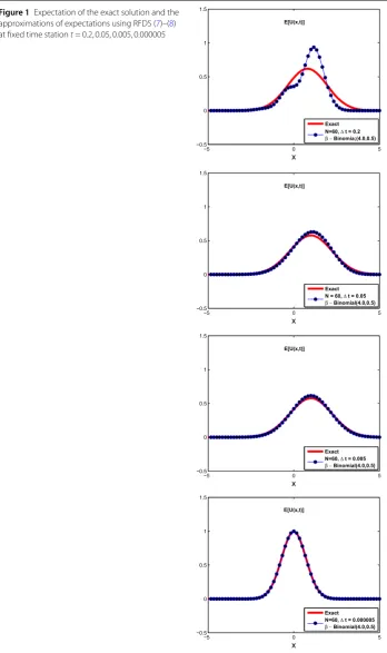
In Fig.1we present a comparison at the time instantt= 0.2, 0.05, 0.005 and 0.000005 (time fixed station) of the expectation of the exact solution s.p. and the approximations of the expectations using the random numerical scheme (7)–(8) with different spatial steps and we note that Fig.1agrees with our calculations.
Figure1indicates that, for fixed expected values of the random variable andxand decreasing the step sizet, we get a more accurate and stable solution to (5).
Also, we can summarize our results from Tables1–4that show the convergence between the first moment of the exact stochastic process solution and the numerical stochastic process approximations.
Additionally, we can confirm the convergence according toλ2as in Tables5–7.
6 Conclusion
We have presented a consistent and stable RFDS that approximates the stochastic solution of the Cauchy advection–diffusion problem with random variable coefficient under mean square and mean fourth calculus.
Acknowledgements
The author is grateful to the anonymous referees for their excellent comments.
Funding
This work was supported by the Mathematics Department—Mansoura University of Egypt.
Competing interests
The author declares that there is no conflict of interests regarding the publication of this article.
Authors’ contributions
The author wrote, read and approved the final manuscript.
Publisher’s Note
Springer Nature remains neutral with regard to jurisdictional claims in published maps and institutional affiliations.
Received: 6 June 2018 Accepted: 31 January 2019 References
1. Øksendal, B.: Stochastic Differential Equations: An Introduction with Applications. Springer, Berlin (2003)
2. Kloeden, P., Platen, E.: Numerical Solution of Stochastic Differential Equations. Applications of Mathematics. Springer, Berlin (1992)
3. Han, H., Huang, Z.: A class of artificial boundary conditions for heat equation in unbounded domains. Comput. Math. Appl.43(6–7), 889–900 (2002).https://doi.org/10.1016/S0898-1221(01)00329-7
4. Wu, X., Sun, Z.Z.: Convergence of difference scheme for heat equation in unbounded domains using artificial boundary conditions. Appl. Numer. Math.50(2), 261–277 (2004).https://doi.org/10.1016/j.apnum.2004.01.001
5. Abdelrahman, M.A.E., Sohaly, M.A.: Solitary waves for the modified Korteweg–de Vries equation in deterministic case and random case. J. Math. Phys.8(1), 214 (2017).https://doi.org/10.4172/2090-0902.1000214
6. El-Tawil, M.A., Sohaly, M.A.: Mean square numerical methods for initial value random differential equations. Open J. Discrete Math.1(2), 66 (2011)
7. El-Tawil, M.A., Sohaly, M.A.: Mean square convergent finite difference scheme for random first order partial differential equations. In: International Conference on Mathematics, Trends and Development ICMTD12, The Egyptian Mathematical Society