Testing for Structural Change

(1)

Testing for Structural Change

Theory, Implementation and Applications

D

ISSERTATION

zur Erlangung des akademischen Grades

eines Doktors der Naturwissenschaften

der Universität Dortmund

Dem Fachbereich Statistik

der Universität Dortmund

vorgelegt von

Achim Zeileis

(2)

Prof. Dr. Walter Krämer (Gutachter) Prof. Dr. Kurt Hornik (Gutachter) Prof. Dr. Götz Trenkler (Gutachter) Dr. Lars Tschiersch (Beisitzer) Tag der mündlichen Prüfung: 14. November 2003

(3)

Danksagung

Nach drei Jahren Arbeit an der Technischen Universität Wien im Rahmen des vom FWF (Fonds zur Förderung der wissenschaftlichen Forschung) geförderten SFB 010 “Adaptive Information Systems and Modelling in Economics and Management Science” habe ich nun die vorliegende Dis-sertation abschließen können. Auch wenn auf dem Umschlag nur mein Name steht, so wäre die Aufnahme, Durchführung und erfolgreiche Beendi-gung ohne die Hilfe und Unterstützung vieler Kollegen und Freunde nicht möglich gewesen.

An erster Stelle gilt mein Dank all denen, die durch gemeinsame Forschung die wissenschaftliche Basis zu dieser Arbeit gelegt haben: Insbesonders möchte ich Kurt Hornik danken, der diese Dissertation betreut hat, mir als wissenschaftlicher Mentor immer zur Seite stand und mir aber auch die Freiheit gelassen hat, meine Forschung nach eigenen Interessen auszurichten. Weiter danke ich Walter Krämer, der mein Interesse für das Themenge-biet dieser Arbeit überhaupt geweckt hat und mich von Beginn meiner Tätigkeit als studentische Hilfskraft an über die Diplomarbeit bis hin zum Abschluß dieser Dissertation unterstützt und mir im Institut für Wirtschafts-und Sozialstatistik an der Universität DortmWirtschafts-und immer eine Anlaufstelle geboten hat. Diese Beziehung von Wien nach Dortmund mit (wissen-schaftlichem) Leben gefüllt hat besonders Christian Kleiber, dem ich für

(4)

sein Engagement und seine in der Regel kritischen aber immer konstruk-tiven Beiträge zu einer sehr angenehmen und produkkonstruk-tiven Forschungsko-operation danke. Bei Friedrich Leisch möchte ich mich dafür bedanken, daß er mir geholfen hat, mich im Alltag des Universitätsgeschäfts zurecht-zufinden. Außerdem bin ich ihm und Kurt Hornik zu Dank verpflichtet, da sie mir nicht nur viel beigebracht haben über wissenschaftliches Ar-beiten im Allgemeinen und über die Umsetzung von statistischen Ideen in informatische Konzepte, sondern mir auch immer eine Plattform zu selb-ständigem Arbeiten geboten haben. Besonders danken möchte ich auch Torsten Hothorn, der in gewisser Weise an der Ausrichtung dieser Arbeit Schuld ist, da ich ohne ihn überhaupt nicht in Wien gelandet wäre. Zu-dem war er auch immer ein guter Diskussionspartner, sowohl für gemein-same wissenschaftliche Projekte als auch für darüber hinausgehende all-gemeinere Fragen.

Für eine angenehme wissenschaftliche Zusammenarbeit sowie streng nicht-wissenschaftliche Aktivitäten abseits des Berufs möchte ich mich bei meinen Wiener Kollegen und Freunden bedanken: Evgenia Dimitriadou, Alexan-dros Karatzoglou und David Meyer haben über die letzten drei Jahre hin-weg unser Büro zu einem Ort gemacht, an dem ich gerne mehr als nur die Arbeitszeit verbracht habe. Auch Bettina Grün, die erst Anfang des Jahres, dazugekommen ist, hat sich sehr gut in diese Atmosphäre einge-fügt und sie bereichert. Ein spezieller Dank geht an Ortrun Veichtlbauer, die nicht nur für eine spannende interdisziplinäre Kooperation verant-wortlich ist, sondern auch mehr als einmal mein seelisches Gleichgewicht zurecht gerückt hat, und ohne dies hätte ich es vielleicht nicht so lang in Wien ausgehalten.

(5)

v Menschen, die mir im Leben außerhalb der Universität Kraft und Rückhalt geben. Deshalb möchte ich all meinen Freunden danken, die mich auch in Zeiten extremer Büroaufenthaltsdauern meinerseits nicht vergessen haben und für mich da waren, um mich an die wichtigeren Dinge im Leben zu erinnern. Das Fundament für all das habe ich aber meiner Familie zu ver-danken, meinen Eltern und meinem Bruder, die mich immer in jeder Hin-sicht unterstützen und ohne die ich nicht da wäre, wo ich heute bin.

(6)

(7)

Abstract

An approach to testing for structural change in parametric models with a special emphasis on (generalized) linear regression models is introduced: First, a generalized framework for testing for parameter instability based on the partial sums of M-estimation equations is presented which allows for testing the stability of parameter coefficients derived from various es-timation techniques like ordinary least squares, maximum likelihood and M-estimation. The core idea of the procedure is to capture the fluctua-tion in the estimating equafluctua-tions and visualize these and asses their sig-nificance. Second, these generalized M-fluctuation tests and virtually all other standard tests for structural change in linear regression models are implemented in a unified framework in the R package strucchange re-flecting the common features of the testing procedures. Third, the useful-ness of the proposed procedures as well as a methodology for recovering the breakpoints of a multiple structural change model are illustrated using several "real world" data sets.

(12)

(13)

Zusammenfassung

Diese Arbeit stellt eine Methode zum Testen auf Strukturbruch bzw. Struk-turveränderung in parametrischen Modellen vor unter besonderer Berück-sichtigung von (verallgemeinerten) linearen Regresionsmodellen: Als er-stes wird eine allgemeine Methode zur Konstruktion von Tests auf Param-eterinstabilität vorgestellt, die auf Partialsummenprozessen von Schätz-gleichungen für M-Schätzer basiert. Diese ermöglichen es, die Stabilität von Parameterschätzungen zu testen, die durch verschiedene Schätztech-niken wie etwa gewöhnliche Kleinste-Quadrate-, Maximum-Likelihood-oder M-Schätzung ermittelt wurden. Die Grundidee des Verfahrens ist es, Prozesse zu berechnen, die die Fluktuation in den zu Grunde liegenden Schätzgleichungen einfängt, diese zu visualisieren und auf signifikante exzessive Fluktuation zu testen, die wiederum auf Parameterinstabiltät schließen ließe.

Als zweites werden diese verallgmeinerten M-Fluktuationstests zusam-men mit nahezu allen anderen Standard-Testverfahren auf Strukturbruch in linearen Regressionsmodellen imR-Paketstrucchange implementiert, das vereinheitlichte Werkzeuge zur Berechnung, Visualisierung und Bes-timmung der Signifikanz der verschiedenen Strukturbruchtests zur Verfü-gung stellt.

Als drittes, wird die Nützlichkeit der behandelten Testverfahren in praxis-3

(14)

nahen Anwendungen illustriert, wo neben den Tests auch Funktionalität zur Schätzung der Anzahl und Zeitpunkte multipler Brüche in linearen Regressionsmodellen vorgestellt wird.

(15)

Chapter 1

Introduction

This monograph is concerned with testing for structural change in para-metric models with a special emphasis on linear regression models: First, the theory for a general class of tests for structural change is established. Second, it is discussed how these and other tests for structural change are implemented in a unified framework reflecting the common properties of the tests in the Rpackage strucchange. Third, the usefulness of the pro-posed procedures in connection with the interface of the implementation is illustrated using applications to several data sets in which the structural changes can be attributed to identifiable historical events.

Before discussing some features and properties of tests for structural change more generally, it should be briefly clarified why we need such tests and implementations and applications for them.

What is a structural change and why should we want to test for it? Struc-tural change is of central interest in many fields of research and data anal-ysis: to learn if, when and how the structure of the data generating mech-anism underlying a set of observations changes. Usually, it is known with

(16)

Time

Annual flow of the river Nile

1880 1900 1920 1940 1960

600

800

1200

Figure 1.1: Annual flows of the river Nile before and after opening of the first Aswan dam

respect to which quantity the structural change might occur, e.g., over time or with the increase of a certain risk factor. One of the simplest examples for such a structural change is a time series whose mean changes at a sin-gle breakpoint. Such a time series is depicted in Figure1.1giving the an-nual discharge of the river Nile at Aswan in 108 m3 before and after the opening of the first Aswan dam in 1898. The plot suggests that the annual flows vary around a constant mean flow in each segment—before 1898 and aftwards—but that there is one break at which the mean flow drops due to the opening of the Aswan dam (in Chapter4it is shown that this is indeed a reasonable model for the data). But to assess whether there is evidence for such a structural change or not, a statistical test is needed: given a model (in the example: constant mean flow) it is tested whether the data support the hypothesis that there is a stable structure against the

(17)

1.1. TESTS FOR STRUCTURAL CHANGE 7 alternative that it changes over time.

Why do we need an implementation of such tests? The obvious first an-swer to this question is, of course, that this is the easiest way to enable potential users to adopt some theoretical results in the analysis of data. Another important issue is the reproducibility of research results: if nu-merical results are given in a scientific article not only the proofs for the theory underlying it should be made available but also the software which produced these results (Leisch 2002). But we would like to stress another point about the implementation of statistical methodology which is often neglected: to a considerable extent software affects how statisticians think about a certain methodology and how they use it in the analysis of data. Therefore, a unified but flexible implementation that reflects the common features of a set of techniques can help practitioners and researchers to un-derstand the underlying theory better and more quickly and to apply the methodology properly and in a more efficient manner.

What are the benefits of applications of the tests? This question is much easier to answer than the previous two. Applications show that the test-ing procedures lead to valuable and interpretable results in the analysis of “real” data. Furthermore, they convey a certain “feeling” for the way the techniques can be used in different situations.

1.1

Tests for Structural Change

Starting from the recursive CUSUM test of Brown, Durbin, and Evans (1975) a large variety of tests for structural change has been suggested in both the econometrics and the statistics literature many of which can be broadly placed into two different classes: generalized fluctuation tests

(18)

(Kuan and Hornik 1995) that do not assume a particular pattern of devi-ation from the hypothesis of parameter constancy and F tests (Andrews 1993;Andrews and Ploberger 1994) that are built for a single shift alterna-tive (of unknown timing).

For a recent review ofFtests for structural change and related techniques seeHansen(2001).

The generalized fluctuation tests fit a parametric model to the data via ordinary least squares (OLS)—or equivalently via maximum likelihood (ML) using a normal approximation—and derive a process which cap-tures the fluctuation of the recursive or OLS residuals (Brown et al. 1975; Ploberger and Krämer 1992; Chu, Hornik, and Kuan 1995a) or the recur-sive or rolling/moving estimates (Ploberger, Krämer, and Kontrus 1989; Chu, Hornik, and Kuan 1995b) and reject if this fluctuation is improba-bly large. In their seminal paper Brown et al. (1975) point out that this framework . . .

“. . . includes formal significance tests but its philosophy is ba-sically that of data analysis as expounded byTukey(1962). Es-sentially, the techniques are designed to bring out departures from constancy in a graphic wayinstead of parametrizing partic-ular types of departure in advance and then developing formal significance tests intended to have high power against these particular alternatives. From this point of view the significance tests suggested should be regarded as yardsticks for the in-terpretation of data rather than leading to hard and fast de-cisions.” (Brown et al. 1975, pp. 149–150)

(19)

1.2. DIAGNOSTIC CHECKING VS. DATA EXPLORATION 9 visualization of fluctuation tests is important, and second, the tests are not only significance tests but also explorative tools.

Instead of capturing the fluctuation in residuals or parameter estimates empirical fluctuation processes can also be based on OLS first order con-ditions or ML scores respectively (Nyblom 1989; Hansen 1992; Hjort and Koning 2002). Although they have not been discussed in the generalized fluctuation test framework (Kuan and Hornik 1995) we show below that they can be seen as an extension of that framework which makes the class of empirical fluctuation processes richer. Furthermore, we show how these ideas can be used in more general situations and employing different esti-mation techniques (not only OLS and ML) under mild assumptions. The resulting class of tests for structural change is based on processes which capture the fluctuation in M-estimating scores.

1.2

Diagnostic Checking vs. Data Exploration

In parametric models structural change is typically described by para-meter instability. If this instability is ignored, parapara-meter estimates are generally not meaningful, inference is severly biased and predictions lose accuracy. AsBreiman(2001) criticizes, parametric data models in general and the linear regression model in particular are used too often without checking the fit of the model to the data: “The linear regression model led to many erroneous conclusions that appeared in journal articles wav-ing the 5% significance level without knowwav-ing whether the model fit the data” (Breiman 2001, p. 203). Furthermore, he argues that it is important to assess the goodness-of-fit of data models not only using omnibus tests but tests designed for a certain direction of the alternative. To avoid using

(20)

non-sense models, a large literature on diagnostic tests and misspecification tests that test the assumptions of the linear regression model emerged in particular in the econometrics community.Krämer and Sonnberger(1986) discuss a collection of tests for diagnostic checking in linear regression re-lationships which are designed for testing the null hypothesis that a stan-dard linear regression model produces an adequate fit for the data against the alternative that one specific assumption is violated, e.g., misspecifica-tion, omitted regressors, functional form, heteroskedasticity or autocorre-lation of the errors, or structural change.

But asBrown et al.(1975) emphasize for the recursive CUSUM test, none of these tests should only be used as pure significance tests but also as ex-plorative tools which can be used to learn about the structure in data. Re-jection of the null hypothesis can not necessarily be regarded as evidence that the particular alternative for which the test is built is true, e.g., struc-tural changes can often also be interpreted as omitted regressors and vice versa, or heteroskedasticity and structural change might be confounded etc. Especially in a structural change framework, it is usually not only of interest to find some model that fits the data (with meaningful para-meter estimates, inference and prediction methods) but also to be able to identify and interpret the structural changes which are of high inter-est for practitioners and researchers. One example for such a situation is the Nile data described above; further examples are discussed through-out the rest of this monograph. Therefore, asZeileis and Hothorn (2002) point out describing the implementation of a collection of diagnostic tests fromKrämer and Sonnberger(1986) in theR packagelmtest, it is always helpful to use diagnostic tests as explorative tools together with diagnostic plots that help to visualize and understand the structure in the data.

(21)

1.3. VISUALIZATION AND SIGNIFICANCE TESTING 11

1.3

Visualization and Significance Testing

AlthoughBrown et al.(1975) stressed that the recursive CUSUM test should bring out departures from parameter instability in a graphic way the vi-sualization of structural change tests was often neglected in the literature although a synthesis of visualization and significance testing offers many advantages. For example,Meyer, Zeileis, and Hornik (2003) discuss how goodness-of-fit testing and visualization of residuals in log-linear mod-els can be combined such that a plot reports unusual observations if and only if the corresponding tests rejects the null hypothesis at some specified level. A similar approach is used below for structural change tests.

More generally, Cleveland (1993) describes the interplay of visualization and probabilistic inference:

“Probabilistic inference is the classical paradigm for data analy-sis in science and technology. [. . . ] Visualization—with its two components, graphing and fitting—is a different paradigm for learning from data. It stresses a penetrating look at the struc-ture of the data. What is learned from the look is guided by knowledge of the subject under study. Sometimes visualization can fully replace the need for probabilistic inference. We visu-alize the data effectively and suddenly, there is what Joseph Berkson called interocular traumatic impact: a conclusion that hits us between the eyes. In other cases, visualization is not enough and probabilistic inference is needed to help calibrate the uncertainty of a less certain issue. When this is so, visual-ization has yet another role to play—checking assumptions.” (Cleveland 1993, pp. 12–14)

(22)

Visualization of structural change tests as introduced in this monograph uses this methodology—fitting of a model to the data and graphing of the fluctuation in residuals, estimates or M-scores—and combines all three purposes: formal significance testing, visualization of the structure of the data and checking the assumption of parameter stability in the underly-ing model. Additionally, the examples discussed throughout this mono-graph illustrate what is called “interocular traumatic impact” above be-cause the plots of fluctuation processes not only visualize the result of the corresponding significance test but also convey rather precise information about the type and number of structural changes.

1.4

Segmentation of Regression Models

Given that there is significant evidence for structural change in some (re-gression) model, a natural approach is to estimate the breakpoints from the data and fit a model to each segment defined by these breakpoints. In several statistical disciplines and communities, methods have been devel-oped that address this problem from different viewpoints. Although the terminology is usually quite different, the corresponding techniques are often strongly related.

In statistical quality control and sequential testing, the detection of such abrupt changes in a sequence of observations has always been an impor-tant topic (see e.g., Siegmund 1985; Basseville and Benveniste 1986; Bas-seville and Nikiforov 1993) which aims at finding out when the underly-ing distribution in this sequence changes as soon as possible and adjust the model correspondingly. In medical research, maximally selected rank statistics are frequently used to estimate cutpoints in some prognostic

(23)

fac-1.5. OVERVIEW 13 tor that splits the sample into two parts and thus serves as a simple binary segmentation rule (Lausen and Schumacher 1992; Hothorn and Lausen 2003). Similar techniques can also be applied recursively with respect to more than one explanatory variable which leads to recursive partitioning and classification and regression trees (Breiman, Friedman, Olshen, and Stone 1984) where usually a constant is fitted to the data in each segment. Instead of segmenting with respect to several variables and fitting simple (constant) models to each segment, another approach is to find change-points with respect to only one variable and fit a more sophisticated model in each segment, e.g., a (generalized) linear regression model (Stasinopou-los and Rigby 1992; Pastor-Barriuso, Guallar, and Coresh 2003). To de-termine the breakpoints in such a model algorithms are needed which minimize the likelihood (Hawkins 2001) or residual sum of squares (Bai and Perron 1998,2003). This is the natural approach in a structural change framework where breaks in a regression model fitted by ML or OLS should be discovered with respect to a unique ordering of the data. If time is the ordering variable this procedure is often called dating of structural changes. We adopt this approach and implement and apply the algorithm ofBai and Perron(2003) in such a way that it reflects the common features of the procedures mentioned above: given evidence for structural breaks, find a segmentation with respect to one ordering variable and then fit a segmented regression model.

1.5

Overview

This monograph presents a theoretically and computationally sound and flexible framework that reflects all the features described above: First,

(24)

it extends the generalized fluctuation test framework (Kuan and Hornik 1995) by introducing fluctuation processes based on M-scores. Second, it describes how (M-)fluctuation tests on the one hand andFtests (Andrews 1993; Andrews and Ploberger 1994) on the other are implemented in a unified way in theRpackagestrucchange. Third, the tests are applied to data sets with a special focus to multiple change models and the recov-ering of the number and location of the breakpoints. More precisely, this monograph is organized as follows: Chapter2 introduces a general class of fluctuation tests for parameter instability which is based on partial sums of M-estimation equations and contains many well-known tests from the generalized fluctuation test framework (Kuan and Hornik 1995) as special cases. Functional central limit theorems which govern the asymptotic be-haviour of the corresponding fluctuation processes under the hypothesis and local alternatives are derived under mild assumptions. A unified ap-proach is outlined to the construction of test statistics and to strategies for combining traditional significance testing with visualization methods for detecting the timing of a potential shift and which parameter is affected by it. Finally, a few applications of the new fluctuation tests are given. The chapter essentially presents the results ofZeileis and Hornik(2003).

Chapter 3 describes the implementation of a large collection of tests for structural change encompassing virtually all commonly used structural change tests in theR packagestrucchange. Usually, standard economet-rics and statistics software packages just implement a few single tests for structural change which do not reflect the common features of the tests and seldom offer automatic visualization of the results. Therefore, the strucchangepackage implements classes of tests (rather than single tests) and unifies the approaches to testing for structural change with tests from

(25)

1.5. OVERVIEW 15 the generalized (M-)fluctuation test framework (Kuan and Hornik 1995; Zeileis and Hornik 2003) and the F test framework (Andrews 1993; An-drews and Ploberger 1994): first a fluctuation process or sequence of F

statistics is computed which then can be plotted together with its bound-aries and finally a significance test can be carried out, including the com-putation of an (approximate) asymptoticpvalue. This connects traditional significance testing with visualization techniques that allow for better un-derstanding of the structure of the data and the decision of the correspond-ing significance test, like motivated above. Furthermore, it is described how incoming data can be monitored online. The chapter mainly gives the results ofZeileis, Leisch, Hornik, and Kleiber(2002).

Chapter 4 applies the introduced methodology for testing for structural change to “real world” data with a special emphasis on multiple structural changes and dating of structural changes in a linear regression setup. In addition to the various testing strategies, a dynamic programming algo-rithm for the estimation of the breakpoints is discussed and implemented in thestrucchangepackage. Using historical data on Nile river discharges, road casualties in Great Britain and oil prices in Germany it is shown that statistically detected changes in the mean of a time series as well as in the coefficients of a linear regression coincide with identifiable historical, political or economic events which might have caused these breaks. The results are essentially those ofZeileis, Kleiber, Krämer, and Hornik(2003).

(26)

(27)

Chapter 2

Generalized M-Fluctuation Tests

for Parameter Instability

2.1

Introduction

The generalized fluctuation test framework (Kuan and Hornik 1995) is one of the important classes of structural change tests as discussed above. Its main idea is to fit a parametric model to the data via OLS—or equiva-lently via maximum likelihood (ML) using a normal approximation—and derive a process which captures the fluctuation in the residuals or para-meter estimates and reject if this fluctuation is improbably large. Using similar principles, tests for parameter instability have been suggested that capture fluctuations in OLS first order conditions or ML scores respec-tively (Nyblom 1989; Hansen 1992; Hjort and Koning 2002). Although these have not been discussed in the generalized fluctuation test frame-work (Kuan and Hornik 1995) we show below that they can be seen as an extension of that framework which makes the class of empirical

(28)

tuation processes richer. In addition, we further unify the fluctuation test framework by showing how under mild assumptions these ideas can be used in more general situations and employing different estimation tech-niques (not only OLS and ML). The resulting class of tests for parameter instability which is based on M-estimation scores contains many of the tests mentioned above as special cases and unifies the approaches to the construction of test statistics. Strategies are outlined for combining tra-ditional significance testing with visualization methods for detecting the timing of a potential structural change and which parameter is affected by it.

All these techniques have in common that it is known with respect to which quantity the instability might occur: e.g., in time series regression it is natural to ask whether the relationship between dependent and ex-planatory variables changes over time. In clinical studies often change-point problems arise where a regression relationship changes with respect to the size of one risk factor etc. The situations described have in common that the observations have some unique ordering with respect to which a structural change occurs but that the (potential) changepoint is unknown. This chapter is organized as follows: in Section2.2we introduce the para-metric model and formulate the null hypothesis before we derive func-tional central limit theorems for partial sum processes of M-scores under the hypothesis of parameter stability and under local alternatives in Sec-tion2.3. The construction of the generalized M-fluctuation tests—from the choice of the estimation technique to the test statistic that captures the fluc-tuation in the M-score processes—is described in Section 2.4. Section2.5 discusses tests based on ML-scores in (generalized) linear models and the usefulness of the proposed tests is illustrated in Section2.6based on data

(29)

2.2. THE MODEL 19 for German M1 money demand, historical demographic time series of ille-gitimate births in in the village of Großarl, Austria, and youth homicides in Boston, USA, in a policy intervention framework.

2.2

The Model

We assumenindependent observations

Yi ∼ F(θi) (i =1, . . . ,n). (2.1)

distributed according to some distributionFwithk-dimensional parameter

θ_i. We also assume that the observations are uniquely ordered by some external variable, usually time. TheYi can possibly be vector valued, ex-tensions to a regression situation whereYi = (yi,xi)>and thexiare some additional covariates are presented later.

We are interested in testing the hypothesis

H0 : θi = θ0 (i =1, . . . ,n) (2.2)

against the alternative that (at least one component of)θ_ivaries over “time”. For this alternative to be sensible the ordering assumption is necessary: If a parameter instability with a single breakpoint, say, occurs with respect to a certain ordering of the variables this single breakpoint interpretation would be lost by re-ordering in such a way that observations from the two regimes are mixed. The assumption of independence is assumed for convenience and will be weakened later.

(30)

2.3

Generalized M-Fluctuation Processes

In this chapter, we suggest a general class of fluctuation processes that can capture instabilities in the parameterθ. In the first two Sections2.3.1and 2.3.2 the fluctuation processes are introduced and their behaviour under the null hypothesis (2.2) is derived. The limiting process is first derived for knownθ₀ and then for the case where it has to be estimated. In Sec-tion 2.3.3, the results are generalized to local alternatives and finally in Section2.3.4some further fluctuation processes are introduced.

2.3.1

Theoretical Fluctuation Processes

Consider some suitably smooth k-dimensional score function ψ(·) (see e.g.,White 1994), independent ofnandi, with

E[ψ(Yi,θi)] = 0 (2.3)

and define the following matrices

A(θ) = E[−ψ0(Y,θ)], (2.4)

B(θ) = COV[ψ(Y,θ)], (2.5)

C(θ) = E[ψ(Y,θ)u(Y,θ)>] (2.6)

whereY ∼F(θ₀),ψ0(·)is the gradient ofψ(·)with respect toθ, andu(·,θ)

is

u(y,θ) = ∂logf(y,θ)

∂θ , (2.7)

and f(·,θ)is the probability density function corresponding toF. Hence,u

is the gradient of the log likelihood with respect toθ, also called Maximum Likelihood (ML) score. The first two matrices A(θ)and B(θ)are standard

(31)

2.3. GENERALIZED M-FLUCTUATION PROCESSES 21 in M-estimation, C(θ) is only needed in Section2.3.3. Note that given ψ

the matrices A(θ)andB(θ)but notC(θ)can be estimated without further knowledge ofFor f respectively as the latter depends on the ML scoreu. Theorem 1 For the cumulative score process given by

Wn(t,θ) = √1 n bntc

∑

i=1 ψ(Yi,θ) (2.8)

and under the assumptions stated above and under H0 the following functional central limit theorem (FCLT) holds:

Wn(·,θ0) d

−→ Z(·),

where Z(·)is a Gaussian process with continuous paths, mean functionE[Z(t)] =

0and covariance functionCOV[Z(t),Z(s)] =min(t,s)·B(θ₀).

Proof:The proof follows by direct application of Donsker’s theorem (Billings-ley 1999).

Corollary 1 If B(θ₀) is non-singular, the following FCLT holds for the decorre-lated fluctuation process

B(θ0)−1/2Wn(·,θ0) d

−→ W(·),

where W(·)is a k-dimensional Wiener process or standard Brownian motion.

2.3.2

Empirical Fluctuation Processes

Usually, in applications the parameterθ0 is not known but has to be

es-timated. A suitable estimator can be based on the functionψ(·): the full sample M-estimator ˆθn is defined by the equation

n

∑

i=1

(32)

Some properties of this M-estimator are well known (see e.g., Stefanski and Boos 2002). Taylor expansion of

Sn(θ) = 1 n n

∑

i=1 ψ(Yi,θ) (2.10) gives 0 = Sn(θˆn) = Sn(θ0) + S0n(θ0)(θˆn−θ0) + Rn. (2.11) Under suitable regularity conditions

−S0_n(θ₀) = 1 n n

∑

i=1 −ψ0(Yi,θ0) p −→ A(θ₀), √ nSn(θ0) d −→ N (0,B(θ₀)), √ nRn p −→ 0.

Therefore, the following holds

√

n(θˆ_n−θ₀) −→d N (0,V(θ₀)), (2.12) where V(θ) = A(θ)−1B(θ){A(θ)−1}>. See Stefanski and Boos (2002) or White (1994) for further details; White (1994, Theorem 6.10, p. 104) also gives a set of suitable regularity conditions. Equivalently to (2.12) we can write

√

n(θˆ_n−θ₀) =· A(θ₀)−1·Wn(1,θ0), (2.13)

where an

·

= bn means that an−bn tends to zero (in probability if an or bn are stochastic).

Theorem 2 Under H0 the following FCLT holds for the empirical cumulative score process with M-estimated parameters

Wn(·, ˆθn)

d

−→ Z0(·),

(33)

2.3. GENERALIZED M-FLUCTUATION PROCESSES 23 Proof: Wn(t, ˆθn) · = √1 n bntc

∑

i=1 ψ(Yi,θ0) + 1 n bntc

∑

i=1 ψ0(Yi,θ0)· √ n(θˆn−θ0) · = Wn(t,θ0)− bntc n A(θ0)·A(θ0) −1_W n(1,θ0) d −→ Z(t)−t·Z(1).

Corollary 2 If B(θ₀) is non-singular, the following FCLT holds for the decorre-lated empirical fluctuation process with M-estimated parameters

ˆ

B−n1/2Wn(·, ˆθn)

d

−→ W0(·),

where W0(·)is a standard k-dimensional Brownian bridge with W0(t) =W(t)− tW(1)andBˆnsome consistent and non-singular covariance matrix estimate, e.g.,

ˆ Bn = 1 n n

∑

i=1 ψ(Yi, ˆθn)ψ(Yi, ˆθn)>. (2.14)

In the following, the empirical fluctuation process is also denoted

efp(t) = Bˆn−1/2Wn(t, ˆθ). (2.15)

2.3.3

Local Alternatives

In parameter instability problems or structural change situations an alter-native of interest is the local alteralter-native

HA : θi = θ0+√1 n g i n , (2.16)

whereg(·)is a function of bounded variation on[0, 1]which describes the pattern of departure from stability of the parameterθ₀(Kuan and Hornik 1995;Hjort and Koning 2002).

(34)

ThenYihas the probability density function f(y,θ_i) =· f(y,θ₀) 1+u(y,θ₀)> √1 n g i n , (2.17) which can be easily derived from first order Taylor expansion of f.

Therefore, under a local alternative like (2.16) the components of the fluc-tuation process (2.8) no longer have zero mean in general but

E[ψ(Yi,θ0)] · = Z ψ(y,θ₀)f(y,θ₀)dy+ (2.18) Z ψ(y,θ₀)u(θ₀)>f(y,θ₀) √1 n g i n dy (2.19) = 0+√1 n C(θ0) g i n . (2.20)

In fact, with the same arguments as in Section 2.3.1and 2.3.2, the whole fluctuation process can be split into one part which is governed by the FCLT from Theorem1and a second part which is determined by the func-tiongfrom (2.16):

Wn(·,θ0) d

−→ ZA(·), (2.21)

whereZA(t) =W(t) +C(θ₀)G(t)and G(·) is the antiderivative ofgwith

G(t) =Rt

0 g(y)dy.

Finally, the following limiting process can be derived for the decorrelated empirical fluctuation process:

ˆ B−n1/2Wn(t, ˆθn) · = Bˆ−n1/2{Wn(t,θ0)−tWn(1,θ0)} (2.22) · = W0(t) +B(θˆ_n)−1/2C(θˆ_n)G0(t), (2.23) withG0(t) =G(t)−tG(1), providedB(·)is consistent underHA.

The results above include the results from Section 2.3.1 and 2.3.2as spe-cial cases because under the null hypothesis of parameter stability (2.2) the function g is identical to zero g ≡ 0. But the results also imply that tests

(35)

2.3. GENERALIZED M-FLUCTUATION PROCESSES 25 based on the empirical fluctuation processes will be consistent against suitable local alternatives of type (2.16).

2.3.4

Other Fluctuation Processes

Instead of capturing the fluctuation in a cumulative sum of scores, a mov-ing or rollmov-ing sum of scores could be used as well. More formally, we also consider processes of type

Mn(t,θ) = √1 n bNntc+bnhc

∑

i=bNntc+1 ψ(Yi,θ), (2.24)

whereNn = (n− bnhc)/(1−h)andhdetermines the bandwidth.

Under H0this process converges to the increments of a Brownian motion

or bridge respectively, depending on whether the valueθ₀is known or has to be estimated. The latter case is stated formally in the following theorem.

Theorem 3 Under H0 the following FCLT holds for the empirical moving score fluctuation process:

ˆ

Bn−1/2Mn(·, ˆθn)

d

−→ M0(·), (2.25)

where M0(t) = W0(t+h)−W0(t)is the process of increments of a Brownian bridge.

Proof:The proof follows by application of Lemma A fromChu et al.(1995a) to the results of Section2.3.2and2.3.1.

(36)

2.4

Generalized M-Fluctuation Tests

2.4.1

Choice of the Scores

ψ

We choose the M-estimation framework for estimation of the parametersθ

as it contains many other estimation techniques as special cases by choos-ing a suitable score functionψ. Other classes of estimators are not strictly special cases but are strongly related to M-estimation and the principles introduced in Section 2.3 can be used to construct fluctuation processes with the same asymptotic properties. A few of these generalizations are outlined in the following.

One of the most common choices for ψis the partial derivative of some objective functionΨ

ψ(y,θ) = ∂Ψ(y,θ)

∂θ , (2.26)

whereΨcould be the residual sum of squares or the Log-Likelihood, yield-ing the OLS or ML estimators ˆθ respectively (the dependence of ˆθ on the number of observations n is ignored in the following). In both cases the cumulative sums of the first order conditionsψlead very naturally to fluc-tuation processes as described in the previous section.

Another estimating approach which is particularly popular in economet-rics is to use a Quasi-Maximum Likelihood (White 1994) in a misspecifi-cation context. This again is similar to M-estimation in robust statistics (Huber 1964, 1972) which also accounts for violation of some of the stan-dard model assumptions.Huber(1964) suggests the function

ψ_H(y,θ) = min(c, max(y−θ,−c)). (2.27) with some constant c for robust estimation of the mean of a symmetric distribution. Note that this function is not smooth but it is almost

(37)

every-2.4. GENERALIZED M-FLUCTUATION TESTS 27 where differentiable (except in±c) and in the definition of the matrixA(θ)

in (2.4) integration and differentiation can be interchanged. Hence, almost identical results for estimation and construction of fluctuation processes can be derived using functions like Huber’sψfrom (2.27).

Another approach is to not fully specify a model via its likelihood but via some estimating equations (Godambe 1960, 1985) which are satisfied by the true model. Similarly, some moment or orthogonality conditions can be exploited to derive estimating functions which again yield parameter estimates. This approach is used in estimation techniques like instrumen-tal variables in linear models (IV, Sargan 1958), the generalized method of moments (GMM,Hansen 1982) for the estimation of economic models or the generalized estimating equations (GEE,Liang and Zeger 1986) for models for longitudinal or time-series data in biostatistics. Further dis-cussion of related estimation approaches can be found in Bera and Bilias (2002). Usually, these are regression models which are not yet covered by the methodology introduced above. However, with some modifications as described in Section2.5fluctuation processes with rather similar prop-erties can be derived.

All these methods have in common that the estimation ofθ is based on some score or estimating functionψor a moment or orthogonality condi-tion similar to (2.9) whose partial sums yield fluctuacondi-tion processes satisfy-ing some FCLT which again can be used to construct tests for parameter instability. The latter step will described in detail in the following section.

(38)

2.4.2

Test Statistics

We derived the empirical fluctuation processes because they can capture departures from the null hypothesis (2.2) of parameter stability. Therefore, visual inspection alone conveys information about whetherH0is violated

or not. But this alone is, of course, not enough and we want to derive tests based on empirical fluctuation processes. One common strategy for this is to consider some scalar functionalλthat can be applied to the fluctuation processes.

Given a finite sample as in model (2.1) an empirical fluctuation process is an n×k matrix (efp_j(i/n))i,j with i = 1, . . . ,n and j = 1, . . . ,k that converges to ak-dimensional limiting process which is continuous in time. To aggregate this empirical process to a scalar test statistic several suitable functionals of the form

λ efp_j i n . (2.28)

are conceivable. The limiting distribution for these test statistics can be de-termined fairly easily, it is just the corresponding (asymptotic) functional applied to the limiting process. Although closed form results for certain functionals of Brownian bridges exist, the critical values are typically best derived by simulation so there are no constraints for the choice ofλ.

λ can usually be split into two components: λ_time which aggregates over time and λcomp which aggregates over the components of ψ. Common

choices forλ_timeare the absolute maximum, the mean or the range (Krämer and Schotman 1992;Kuan and Hornik 1995;Hjort and Koning 2002;Zeileis et al. 2002). Typical functionalsλ_comp include the maximum norm (or L∞

norm, denoted as|| · ||_∞) or the squared Euclidian norm (or L2 norm,

de-noted as|| · ||2

(39)

2.4. GENERALIZED M-FLUCTUATION TESTS 29 As the decorrelated processes are asymptotically independent it seems to be more intuitive to first aggregate over time and then havekindependent univariate test statistics, each associated with one component of the pro-cess which can usually be matched with one component of the parameter vectorθ. If the overall hypothesis is rejected the component(s) ofθ which caused the instability can then be identified.

On the other hand, when there is evidence for a structural change a very natural question is whenit occured. To focus on this question it is obvi-ously better to first aggregate over jand then inspect the resulting univari-ate process for excessive fluctuation which can be also done visually, e.g. by checking whether this process crosses some boundary b(t) = c·d(t). In this case c determines the significance level and d(·) the shape of the boundary and the resulting test statistic is

max i=1,...,n λcomp efp_j(i/n) d(i/n) , (2.29)

i.e., a weighted maximum of the absolute values of the process aggre-gated by λcomp. Natural choices are to weigh all observations equally,

i.e., d(t) = 1, or by the (asymptotic) standard deviation of the fluctua-tion process, i.e.,d(t) = pt(1−t) for the cumulative score process. But other boundaries are also conceivable, seeZeileis(2004) orZeileis, Leisch, Kleiber, and Hornik(2004) for a more detailed discussion.

The only class of test statistics which allows for both identification of the component jas well as the timing i/nof a potential structural instability is when the maximum is used for aggregating over both time and compo-nents, i.e., max i=1,...,n j=max1,...,k efp_j(i/n) d(i/n) (2.30)

(40)

where the efp_j(i/n) which cross some absolute critical value c can be re-garded as violating the hypothesis of stability (Mazanec and Strasser 2000).

2.4.3

Special Cases

The rich class of generalized M-fluctuation tests introduced in this chapter contains various tests for parameter instability or structural change known from the statistics and econometrics literature.

ML scores: Most importantly, the generalized M-fluctuation tests contain the tests of Hjort and Koning(2002) who develop a general class of fluc-tuation processes based on the ML scores from (2.7). These yield the ML estimate ofθ0 and A(θ0) = B(θ0) = C(θ0) = I(θ0) is the usual Fisher

information matrix. Hjort and Koning (2002) illustrate how to construct three types of tests which are all included in the more general framework above. In particular they construct a Cramér-von Mises type test which is the average of the Euclidian norm of the fluctuation process at time t. However, they do not point out that this is the test ofNyblom(1989) which Hansen (1992) generalized to linear regression models. Nyblom (1989) showed that this test is locally most powerful against the alternative that the parameters follow a random walk.

Changes in the mean: In the case that the Yi are (not necessarily normally) distributed with meanµ₀ and varianceσ2 various tests for the constancy of the mean can be shown to be special cases of the approach presented above: if µ₀ is estimated by means of OLS the OLS-based CUSUM test (Ploberger and Krämer 1992) and the recursive estimates test (Ploberger et al. 1989) are both equivalent to the natural test resulting from the ideas described above: derive the partial sum process of the scores from

(41)

Corol-PARAMETER INSTABILITY IN GLMs 31 lary2and reject if the maximum absolute value of the process—which is just the scaled cumultative sum of the OLS residuals—is too large. With boundaries proportional to the standard deviation the resulting test is the alternative OLS-based CUSUM test ofZeileis (2004) and with moving in-stead of cumulative sums as in (2.25) the resulting process is equivalent to the OLS-based MOSUM process (Chu et al. 1995a) and the moving esti-mates process (Chu et al. 1995b). Krämer and Schotman(1992) andKuan and Hornik(1995) also consider tests based on the range instead of max-imum absolute value for the same processes. If robust M-estimation in-stead of OLS is used for estimatingµ₀tests like the (non-recursive) robust CUSUM tests ofSen(1984) orSibbertsen(2000) can be constructed.

The connection between the generalized M-fluctuation tests and the OLS-based CUSUM test and the Nyblom-Hansen test (Cramér-von Mises type test) respectively in a linear regression framework will be described in more detail in the following section.

2.5

Testing for Parameter Instability in

(Gener-alized) Linear Regression Models

The general framework for constructing fluctuation processes and tests based on M-scores presented in the first sections of this chapter is already extremely useful for testing the constancy of model parameters over time; but to explain the generality of the approach without too much technical overhead two assumptions which do not really restrict the generality of the results have been made for convenience. These will be weakened in this Section. First, the observations were assumed to be independent—

(42)

an assumption which is likely to be violated in time series applications but which can usually be overcome easily as shown at the end of this sec-tion. Second, the probability density function f(yi,θi) was assumed to describe the full distribution of theYi—but if the observations can be split into Yi = (yi,xi)> with a response or dependent variable yi and addi-tional regressors or covariates xi the usual approach is to model the con-ditional distribution f(yi | xi,θi) given the xi. The common assumption is that the xi form a weakly dependent process without deterministic or stochastic trends, seeAndrews(1993) for technical details or alsoHansen (1992) or Hjort and Koning (2002). Under such suitable assumptions the same asymptotic distribution can be derived for the processes based on estimates of the regression coefficients which can be obtained by various procedures as discussed in Section2.4.1.

To make the dependence on the covariates obvious the score functionψ

from (2.3) is now written as

ψ(Yi,θi) = ψ(yi,xi,θi). (2.31) Of course, it is still required to have zero expectation (with respect to

f(yi | xi,θi)) which is not difficult to obtain, more crucial is the assumption that the variances stabilize:

1 n n

∑

i=1 COV[ψ(yi,xi,θ0)] = Jn p −→ J, (2.32)

where the matrix J in a regression context corresponds to B(θ) from (2.5) in the no-covariate context. This follows for example from the weak de-pendence assumption stated above.

It is easy to show that functional central limit theorems similar to Theo-rem 1 and 2 hold for the resulting theoretical and empirical fluctuation

(43)

PARAMETER INSTABILITY IN GLMs 33 processes based onψ(yi,xi,θi), in particular the limiting processes are the same with J instead of B(θ₀). In the following, two important classes of regression models—the general linear model (LM) and the generalized lin-ear model (GLM)—are treated in more detail.

2.5.1

The General Linear Regression Model

Consider the general linear regression model

yi = x>i β + ui (i=1, . . . ,n), (2.33) where the disturbances have zero mean and common varianceσ2. The precise formulation of these assumptions is not important as long as they imply the same FCLT—for different sets of assumptions see, e.g.,Hansen (1992), Andrews (1993), Ploberger and Krämer (1992) or Bai (1997a). To simplify notation and to emphasize common properties of the scores in the LM and the GLM the mean of the yiis sometimes denoted byµi =x>_i β. The model parametersθ = (β,σ2)> are usually estimated by OLS or ML (based on a normal model) which is both equivalent to using the following scores (summands of the first order conditions in an OLS framework):

ψ(yi,xi,θ) = ψβ(yi,xi,β),ψσ2(y_i,x_i,β,σ2) > , (2.34) ψβ(yi,xi,β) = xi(yi−xi>β) = xi(yi−µi), (2.35) ψ_σ2(y_i,x_i,β,σ2) = (y_i−x>_i β)2−σ2. (2.36)

These give the usual estimates ˆβand ˆσ2. In a normal model the two es-timates are independent and thus the covariance matrixJn corresponding toψ(·)from (2.34) is block diagonal

Jn = σ2   1 n∑ni=1xix>_i 0 0 2σ2  .

(44)

Therefore, independent test statistics for the constancy ofβandσ respec-tively can be computed and the stability of the parameters can be assessed independently.

Three test statistics will be derived in the following: the Nyblom-Hansen test, the double max test and the OLS-based CUSUM test.

Nyblom-Hansen test: We follow the approach of Hansen (1992) and test both parametersθ = (β,σ2)> simultanously. In his equation (9) he gives the formula for the test statisticLC based on the following empirical fluc-tuation process and covariance estimate

Wn(t, ˆθ) = √1 n bntc

∑

i=1 ψ(yi,xi, ˆθ), (2.37) ˆ J = 1 n n

∑

i=1 ψ(yi,xi, ˆθ)ψ(yi,xi, ˆθ)>. (2.38) The test statisticLC is then given as

LC = 1 n n

∑

i=1 Wn i n, ˆθ > ˆ J−1Wn i n, ˆθ = 1 n n

∑

i=1 efp i n > efp i n = 1 n n

∑

i=1 efp i n 2 2 ,

which can be interpreted easily as described in Section2.4.2. The asymp-totic distribution isR1

0 ||W0||22, whereW0is ak-dimensional Brownian bridge.

Nyblom(1989) first suggested this test in a structural change context and showed that it is locally most powerful for the alternative that the param-eters follow a random walk. Without relating to Nyblom’s earlier work, Hjort and Koning (2002) refer to it as a Cramér-von Mises type test, but they also point out that visual inspection of the processefp(t) might con-vey information about the timing of a potential structural change.

(45)

Al-PARAMETER INSTABILITY IN GLMs 35 though enhancing classical significance testing by visual means is a good idea, this approach has the problem that what is tested and what is vi-sualized differ. From the transformation above it becomes clear that it is much more natural to use a plot of ||efp(t)||2

2 with two horizontal lines,

one for the empirical mean and one for the critical value which visualizes both the significance test and excessive fluctuation (i.e., information about the timing of the shift). An example for this fluctuation process and its visualization is given in Section2.6.1.

Doublemaxtest: As mentioned in Section2.4.2the only test statistic which allows the identification of both the timing of a structural change and the component of the parameter vectorθwhich has changed is

max

j=1,...,k0max≤t≤1|efpj(t)|, (2.39)

which is the same functional for measuring excessive fluctuation as in the recursive estimates test (Ploberger et al. 1989). The limiting distribution is maxj=1,...,k||W_j0(t)||∞. Again, this test can also be performed graphically by plotting each individual process with a horizontal boundary for±the critical value.

OLS-based CUSUM test: As already indicated in the previous section, the OLS-based CUSUM test for a change in the mean (without covariates) can be shown to be a special case of the the generalized M-fluctuation test framework. In the regression setup this means that there is one constant regressor xi ≡ 1 and the varianceσ2 is treated as a nuisance parameter. If we consider the OLS-based CUSUM test for a setup with covariates another interesting interpretation emerges from the M-fluctuation view. If an intercept is included in the regression, the OLS-based CUSUM pro-cess is equivalent to the first component of the non-decorrelated propro-cesses

(46)

Wn(t, ˆθ) from (2.37) standardized by ˆσ2 which is element(1, 1) of the es-timated covariance matrix ˆJ. Thus, whereas the first component of the decorrelated fluctuation process ˆJ−1/2Wn(t, ˆθ)captures instabilities of the intercept the first component of the non-decorrelated fluctuation process

Wn(t, ˆθ) captures instabilities in the (expected) mean E[x]>β. The latter point is proved formally inPloberger and Krämer (1992). This result im-plies that shifts orthogonal to the mean regressor E[x]cannot be detected using fluctuation processes based on residuals as such shifts can be inter-preted to change the variance rather than the (expected) mean. If the mean

L2norm rather than the L∞ norm is used (as in the Nyblom-Hansen test)

to measure excessive fluctuation in the OLS-based CUSUM process the re-sulting test is also trend-resistant, i.e., can deal with trending regressors (Ploberger and Krämer 1996).

2.5.2

The Generalized Linear Regression Model

Now consider the generalized linear model (GLM) like inMcCullagh and Nelder (1989). To fix notation, yi is a response variable distributed in-dependently according to a distribution F(θ,φ) whereθ is the canonical parameter andφis the dispersion parameter common to allyi. The prob-ability density has the form

f(yi |θ,φ) = exp yiθ−q(θ) w(φ) +p(yi,φ) , (2.40)

for some known functions p(·), q(·) and w(·), so that E[yi] = µi = q0(θ) and VAR[yi] = w(φ)q00(θ) = w(φ)V(µi).

The following relationship is assumed for covariates and responses:

(47)

PARAMETER INSTABILITY IN GLMs 37 where h−1(·) is a known link function,βis again the vector of regression coefficients andη_iis the linear predictor.

The regression coefficientsβare usually estimated by ML andφis treated as a nuisance parameter (or is known anyway). The resulting score func-tion forβis

ψ(yi,xi,β) = xi h0(x>i β) V(µi)−1(yi−µi), (2.42) whereh0(·)is the derivative of the inverse link funtion. The corresponding covariance matrixJn is given by

Jn = 1 n n

∑

i=1 h0(x>_i β)2w(φ) V(µ_i)−1xix>i . (2.43) In the following, we give explicit formulae for the empirical fluctuation processes in two important special cases of the GLM: the binomial (logis-tic) regression model and the log-linear poisson model.

Binomial model:Letyibe the proportion of successes frommtrials such that

myi is binomially distributed Bin(µi,m). Then the variance is determined byw(φ) = 1/mandV(µ) =µ(1−µ)and if the canonical logit link is used then h0(x) = exp(x)/(1+exp(x))2. Given the ML estimates ˆβ and the corresponding fitted values ˆµ_i, the covariance matrix for the M-fluctuation process can be estimated by

ˆ J = 1 nm n

∑

i=1 h0(x>_i βˆ)2 ˆ µ_i(1−µˆ_i)xix > i . (2.44)

The empirical fluctuation process is then given by

efp(t) = Jˆ−1/2√1 n bntc

∑

i=1 h0(x>_i βˆ) yi−µˆi ˆ µ_i(1−µˆ_i)xi. (2.45)

Corresponding test statistics could be derived by, e.g., taking again the av-erage Euclidian norm or the double maximum etc. Note that this method-ology can also be applied if m = 1 where at each timei there is only one

(48)

observation of success (yi = 1) or failure (yi = 0). Applications of this process in a binomial model can be found in Section2.6.2and2.6.3.

Poisson model: If theyi are poisson distributed Poi(µi)thenV(µ) =µand

w(φ) = 1. Using the canonical log link yields h0(x) = exp(x) so that the covariance can be estimated by

ˆ J = 1 n n

∑

i=1 ˆ µ_ixixi>. (2.46) The empirical fluctuation process which is also given inHjort and Koning (2002) simplifies to efp(t) = Jˆ−1/2√1 n bntc

∑

i=1 (yi−µˆi)xi (2.47) and test statistics can be computed like above. As pointed out for the OLS-based CUSUM test in Section2.5.1a test for changes in the mean the first component of the non-decorrelated process can also be used alone which has to be standardized by element (1,1) of the covariance matrix. For the poisson model this gives

efp(t) = √1 n n

∑

i=1 yi_√−µˆi ¯ µ , (2.48)

where ¯µis the arithmetic mean of the fitted values ˆµ_i. If the variances are constant, i.e., if there is only a constant regressor xi ≡ 1 this is a CUSUM process based on the Pearson residuals. If not, it is almost a Pearson resid-uals CUSUM process except that the variance is estimated by ¯µrather than

ˆ

µ_i. The latter is not possible if ˆµ_i is not consistent for the asymptotic vari-ance, that is, the variance has to be estimated from a set of observations and the size of this set has to go to infinity withn. This Pearson residual-based CUSUM process is applied to a Poisson model in Section2.6.4. With a simple modification both processes can not only be used in pois-son but also in quasi poispois-son models where overdispersion is allowed.

(49)

PARAMETER INSTABILITY IN GLMs 39 Then, the variance is not required to be equal to the mean but can be VAR[yi] = φµi. Note that in this case the density function is not given by (2.40) with w(φ) = φ. The dispersion parameter is a nuisance para-meter and can be consistently estimated by X2/(n−k), where X2 is the usual Pearson χ2 statistic. To obtain properly standardized fluctuation processes,efp(t) from (2.47) or (2.48) respectively has to be multiplied by 1/pφˆ which can then be used as usual for testing the constancy of the regression coefficientsβ.

2.5.3

Dependent Data

As stated above, the assumption of independent observations is often (but not necessarily) violated, in particular when dealing with time series data. Several approaches are conceivable when the methodology introduced above is to be applied to dependent data.

When using ML estimation techniques the parameters can be estimated from a fully specified likelihood or from a conditional likelihood and the fluctuation processes can be derived accordingly. But in many situations this is not necessary as consistent estimates ˆθ (or ˆβ in regression frame-works) can be obtained from the usual estimating equations (Godambe 1985; Liang and Zeger 1986). But as Lumley and Heagerty (1999) point out, it is crucial for inference in such models to compute consistent esti-mates for the covariance matrix ˆB(or ˆJrespectively in regression models). Lumley and Heagerty(1999) suggest a class of weighted empirical adap-tive variance estimators which are consistent in the presence of correlation in the data. These can be plugged into the fluctuation processes described above which renders the asymptotic theory valid again.

(50)

2.6

Applications

We illustrate a few of the tests discussed above by applying them to the following four models: an error correction model (ECM) for German M1 money demand, a binomial GLM for the fraction of illegitimate births in Großarl and for simulated binary data and a Poisson model for the num-ber of youth homicides in Boston. The three “real world” data sets are included in the package strucchange implemented in the R system for statistical computing which are both presented in much more detail in the following chapter.

2.6.1

German M1 Money Demand

Lütkepohl, Teräsvirta, and Wolters(1999) investigate the stability and lin-earity of a German M1 money demand function and find a stable rela-tionship for the time before the German monetary unification on 1990-06-01 but a clear structural change afterwards. They used seasonally un-adjusted quarterly data from 1961(1) to 1995(4) for the logarithm of real M1 per capita mt, the logarithm of a price index pt, the logarithm of the real per capita gross national product yt and the long-run interest rate

Rt. The data were originally provided by the German central bank and are now available on the World Wide Web in the data archive of the Jour-nal of Applied Econometrics(http://qed.econ.queensu.ca/jae/1999-v14. 5/lutkepohl-terasvirta-wolters/).

Lütkepohl et al. (1999) used smooth transition regression to model the parameter instability; Zeileis et al. (2004) discuss this model in a struc-tural change framework, but only based on OLS residuals and estimates not based on M-scores. We use the adapted model ofZeileis et al. (2004)

(51)

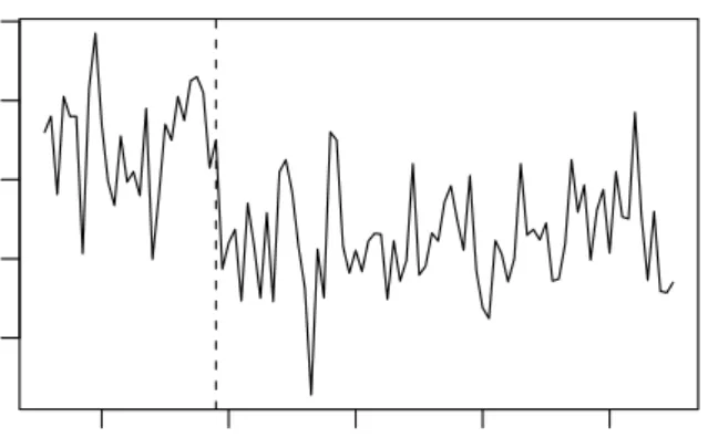
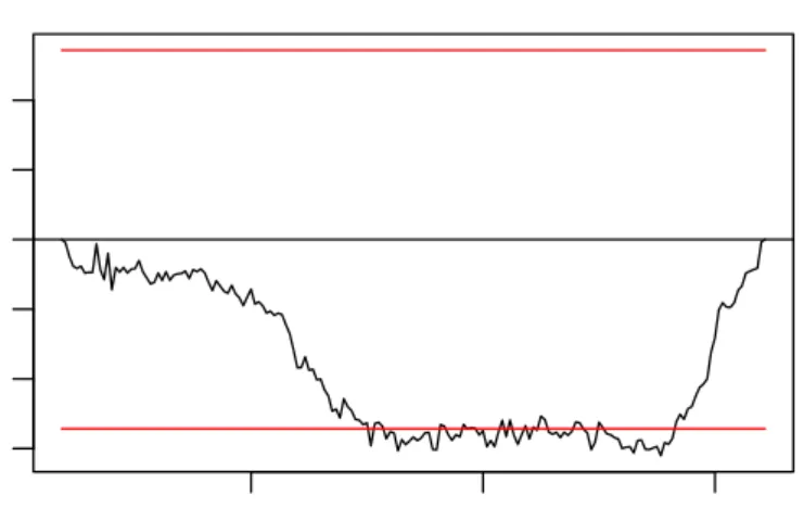
2.6. APPLICATIONS 41 for the German M1 money demand to test the stability of the full sample estimates. Figure2.1shows theL2norm of the score-based fluctuation

pro-cess defined by (2.37) and (2.38) as discussed in Section2.5.1. The dashed horizontal line represents the mean L2 norm||efp(t)||2₂, i.e., the test

statis-tic of the Nyblom-Hansen test, which exceeds its 5% cristatis-tical value (solid line). Additionally to the information that the test finds evidence for struc-tural change in the data, the clear peak in the fluctuation process conveys the information that the break seems to have occured in about 1990, corre-sponding to the German monetary unification (highlighted by the dotted vertical line). The correspondingpvalue is 0.022.

Time

empirical fluctuation process

1960 1970 1980 1990 0 1 2 3 4 5 6 7

Figure 2.1: Score-based fluctuation process (mean L2 norm) for German

(52)

2.6.2

Illegitimate Births in Großarl

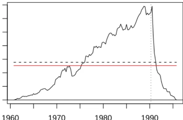
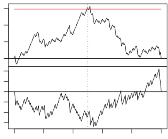
In 18th century Salzburg, Austria, the reproductive behaviour was con-fined to marital unions due to sanctions by the catholic church and the le-gal system. Nevertheless, illegitimate births happened although the catholic church tried to prevent them by moral regulations of increasing sever-ity. Veichtlbauer, Hanser, Zeileis, and Leisch(2002) discuss the impact of these and other policy interventions on the population system in Großarl, a small village in the Austrian Alps in the region of the archbishopric Salzburg. Zeileis and Veichtlbauer (2002) model the structural breaks in the annual fraction of illegitimate births (see Figure2.2) by means of OLS.

Time

Fraction of illegitimate births

1700 1720 1740 1760 1780 1800 0.0 0.1 0.2 0.3 Time

empirical fluctuation process

1700 1720 1740 1760 1780 1800 −1 0 1 2 3

Figure 2.2: Illegitimate births in Großarl and the binomial CUSUM pro-cess

Here, we discuss the number of illegitimate and legitimate births between 1700 and 1800 in a binomial regression framework which is more appro-priate for this kind of data (although the fitted values are equivalent for a regression on a constant). There were about 55 births per year in Großarl

(53)

2.6. APPLICATIONS 43 during the 18th century—about seven of which were illegitimate—with an IQR of (48, 63). During this time the close linkage between religios-ity and moralreligios-ity and between church and state led to a policy of moral suasion and social disciplining, especially concerning forms of sexuality that were not wanted by the catholic church. Moral regulations aimed ex-plicitely at avoiding such unwanted forms of sexuality, e.g., by punishing fornication by stigmatising corrections, corporal punishment, compulsory labour or workhouse-prison. Women sometimes even had to leave the court district afterwards to avoid recidivism. After secularisation such regulations were abolished in the 19th century. To assess whether such in-terventions have any effect on the mean fraction of illegitimate births we employ the CUSUM test based on ML-scores from a binomial model as de-fined in Equation (2.45). The resulting empirical fluctuation process in Fig-ure2.2clearly exceeds its boundary and therefore provides evidence for a decrease in the fraction of illegitimate births suggesting that the moral reg-ulations have been efficient. The peak in the process conveys that there has been at least some structural break at about 1750, but two minor peaks on the left and the right can also be seen in the process. These match very well with the three major moral interventions in 1736, 1753 and 1771 respec-tively (indicated by dotted lines). The correspondingpvalue is<0.0001.

2.6.3

Artificial Binary Data

To show that the approach of M-fluctuation processes is not only applica-ble in situations like above where also OLS estimation techniques could be used despite a binomial GLM being more appriopriate, we analyse an ar-tifical data set of binary observations with covariates. We simulaten =200 observations from a binomial GLM as described in Section2.5.2with the

(54)

canonical logit link. At each time i the response variable is only m = 1 observation of success (yi =1) or failure (yi =0) and the vector of covari-ates isxi = 1,(−1)i

>

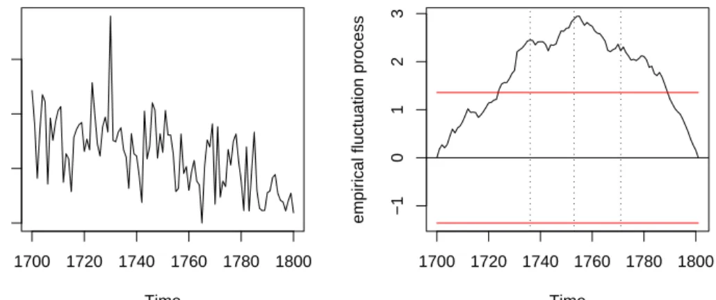
. A single shift model with changepointt =0.5 is used, i.e., 100 observations in each segment, and the vector of regression coefficients in segment 1 isβ_A = (1, 1)>which changes toβB = (0.2, 1)> in segment 2. Thus, the model corresponds to alternating success prob-abilityµ_i = 0.5 and 0.881 in the first segment which drop to alternating success probabilities of 0.31 and 0.769 in the second segment. As only the first regression coefficient but not the remaining one changes this type of alternative is also called partial structural change. Unlike the previous ex-ample, the inspection of the raw time series data in Figure 2.3 does not shed much light on whether or not there has been a change in the param-eters of the underlying model.

● ●● ●●●●●●● ● ● ● ●●● ● ●●●●●●●●●●● ● ●●● ●●● ● ● ●●● ●● ●● ● ●●● ● ●●● ● ● ● ●●● ● ● ● ● ● ●●●●● ● ●●●●●● ●● ● ● ●●●●●●●●●●●●● ● ● ● ●●●●● ● ●● ●● ● ●●● ●●● ● ● ● ● ● ●●● ● ● ● ●●● ● ● ●●● ●●● ● ● ●●● ● ● ● ● ● ●● ●● ● ● ●●● ● ● ●●● ● ●●● ● ●●● ●●● ● ● ●●●●● ● ● ● ● ● ●●● ● ●●● ● ● ● ●●● ● ● ●● ● ● Time y 0.0 0.2 0.4 0.6 0.8 1.0 0 1

Figure 2.3: Artificial binary data

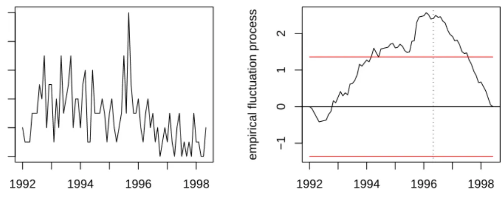
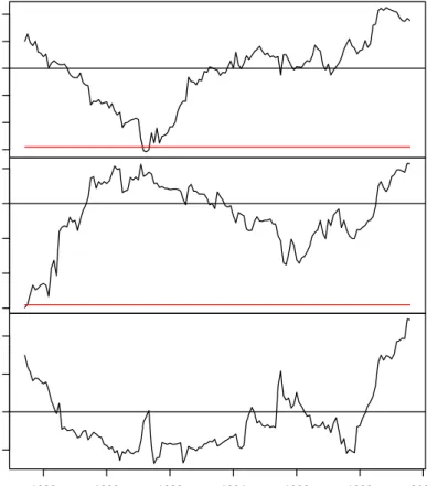
However, if the empricial fluctuation process from Equation (2.45) is de-rived the structural instability can clearly be seen as in Figure2.4. It

(55)

de-2.6. APPLICATIONS 45 picts the 2-dimensional fluctuation process with the boundary and pro-cess for the intercept in the upper panel and the propro-cess for the covariate

(−1)iin the lower panel. This corresponds to using the double max statis-tic from (2.39) which allows for both identification of the instable para-meter and the timing of the shift as discussed in Section2.4.2. As only the first process crosses its boundary the test is able to pick up that the partial break is only associated with the intercept, while the moderate fluctuation of the second process reflects that the corresponding regression coefficient remains constant. The peak in the middle of sample period matches the true breakpoint of t = 0.5 (dotted line) very well. In addition, the fluctu-ation processes in Figure2.4illustrate that although the response variable is just binary the functional limit theorem works very well. The p value

0.0 0.5 1.0 1.5 (Intercept) −0.6 0.0 0.4 x 0.0 0.2 0.4 0.6 0.8 1.0 Time

(56)

corresponding to the double max test is 0.029.

Further discussion of structural changes in historic demographic time se-ries of births and deaths can be found in Veichtlbauer et al. (2002) and Zeileis(2001).

2.6.4

Boston Homicide Data

To address the problem of continuing high homicide rates in Boston, in particular among young people, a policing initiative called the “Boston Gun Project” was launched in early 1995. This project im