c
BAYESIAN EMPIRICAL LIKELIHOOD FOR QUANTILE REGRESSION
BY
YUNWEN YANG
DISSERTATION
Submitted in partial fulfillment of the requirements
for the degree of Doctor of Philosophy in Statistics
in the Graduate College of the
University of Illinois at Urbana-Champaign, 2011
Urbana, Illinois
Doctoral Committee:
Professor Xuming He, Chair
Professor Yuguo Chen
Professor Roger Koenker
Professor Stephen Portnoy
Abstract
Bayesian inference provides a flexible way of combiningg data with prior information. However, quantile regression is not equipped with a parametric likelihood, and therefore, Bayesian inference for quantile regression demands careful investigations. This thesis considers the Bayesian empirical likelihood approach to quantile regression. Taking the empirical likelihood into a Bayesian frame-work, we show that the resultantposterior is asymptotically normal; its mean shrinks towards the true parameter values and its variance approaches that of the maximum empirical likelihood esti-mator. Through empirical likelihood, the proposed method enables us to explore various forms of commonality across quantiles for efficiency gains in the estimation of multiple quantiles. By using an MCMC algorithm in the computation, we avoid the daunting task of directly maximizing empir-ical likelihoods. The finite sample performance of the proposed method is investigated empirempir-ically, where substantial efficiency gains are demonstrated with informative priors on common features across quantile levels.
Acknowledgments
I would never have been able to finish my dissertation without the support of many people. Thus my sincere gratitude goes to my advisor, my committee members, my parents, all my friends, and my companions and superiors for their guidance, support, and patience over the last few years.
I would like to express my deepest gratitude to my advisor, Professor Xuming He, for his excellent guidance, constant encouragement and generous support. Working with Professor He is one of the most important and formative experiences in my life. I feel so lucky to have the opportunity to work with him. I benefit a lot from his patient advising, excellent lectures, frequent meetings and enlightening discussions.
I am also very grateful to my committee members: Professors Yuguo Chen, Roger Koenker, and Stephen Portnoy, who have generously given their time and expertise to better my work. I would like to express my sincere appreciation to them for their insightful suggestions and constant support. I would like to thank Professor Adam T. Martinsek, Dr. Maria Muyot and Professor Annie Qu for the opportunity to work in Illinois Statistics Office. I learned a lot from working with them.
I would also like to thank all the faculties, staff and aluminies in the Statistics Department. Special thanks to Professors Feng Liang and Xiaofeng Shao for their kind suggestions on my work. My thanks must also goes to Professor Ying Wei, Mi-Ok Kim, Huixia Wang, and Dr. Yujun Wu for their kind help on my research and career development.
I am also very grateful to the fellow many graduate students in the Statistics Department, who have shared their memories and experiences. Special thanks to Zhi He, Jing Xia, Yang Feng, Peng Wang, Na Cui, Juan Shen, Yahui Hsu, Ji Yeon Yang, Ji Young Kim, Xingdong Feng and Erin Condon.
Most importantly, I would like to thank my parents for their ultimate love and care during my long years of education. Without your support, I could not be the person as I am today.
Table of Contents
List of Tables . . . vii
Chapter 1 Introduction and Review . . . 1
1.1 Introduction to quantile regression . . . 1
1.2 Review on inference for quantile regression . . . 2
1.3 Introduction to empirical likelihood . . . 5
1.4 Empirical likelihood for quantiles . . . 7
1.5 Empirical likelihood and some other nonparametric inference approaches . . . 9
1.6 Bayesian empirical likelihood for quantile regression (BEL) . . . 11
Chapter 2 Computation . . . 17
2.1 The modified Newton-Raphson algorithm for calculation of empirical likelihood . . . 17
2.2 Bayesian Computation . . . 20
Chapter 3 Properties of the Maximum Empirical Likelihood Estimate (MELE) 22 3.1 Introduction . . . 22
3.2 Properties of the estimating functions in quantile regression . . . 23
3.3 Consistency of the maximum empirical likelihood estimate (MELE) . . . 24
Chapter 4 Asymptotics for the Bayesian Empirical Likelihood . . . 29
4.1 Introduction . . . 29
4.2 Asymptotic property of the posterior distribution . . . 29
4.2.1 Asymptotic property of the posterior distribution with fixed priors . . . 31
4.2.2 Asymptotic property of the posterior distribution with shrinking priors . . . 34
4.3 Discussion . . . 37
4.3.1 Asymptotic theorem with fixed priors: Theorem 4.2.1 . . . 37
4.3.2 Bayesian quantile regression with other working likelihoods . . . 41
Chapter 5 Simulation Studies . . . 45
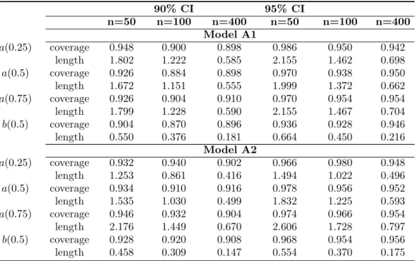
5.1 Coverage properties of the posterior credible intervals . . . 46
5.1.1 Simulation study 1: BEL.s using nearly flat priors . . . 46
5.1.2 Simulation study 2: BEL.s using informative priors . . . 49
5.1.3 Simulation study 3: BEL.c for multiple quantiles estimation . . . 51
5.2 Estimation efficiency of the BEL estimates at quartiles . . . 51
5.2.1 Simulation study 4: estimation efficiency with homoscadestic errors . . . 52
5.2.2 Simulation study 5: estimation efficiency with heteroscadestic errors . . . 54
5.3 Estimation efficiency of the BEL estimates at high quantiles . . . 57
5.3.1 Simulation study 6: models with only one covariate . . . 58
5.3.2 Models with two covariates . . . 60
5.4 Summary on the simulation studies . . . 62
5.5 Discussion . . . 64
Chapter 6 A Real Data Example . . . 69
Chapter 7 Bayesian Quantile Regression with Spatially Correlated Data . . . . 73
7.1 Model introduction . . . 73
7.2 Computation . . . 76
7.3 Asymptotic properties . . . 76
List of Tables
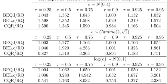
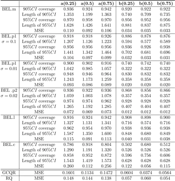
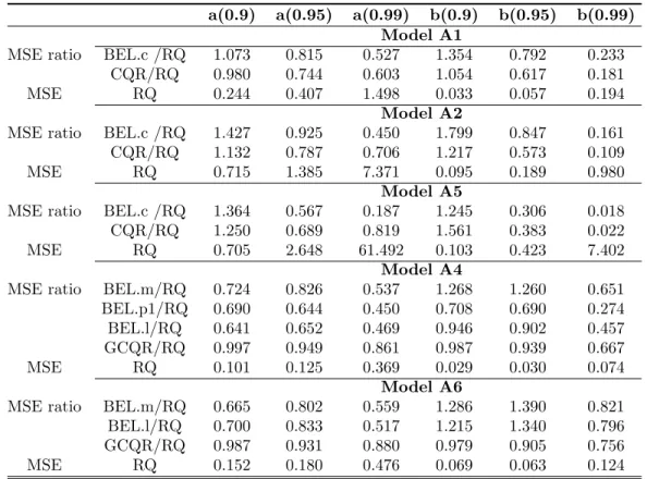
4.1 The table presents the ratio of the asymptotic MSE of the RQ estimators over that of the BEL.l, BEL.c or CQR estimator for Model (4.20) with different error distribu-tions, when jointly estimating quantiles atτ = 0.25,0.5,0.75 andτ= 0.9,0.925,0.95, respectively. . . 41 5.1 Comparison of 95% posterior intervals of the median regression parameters from three
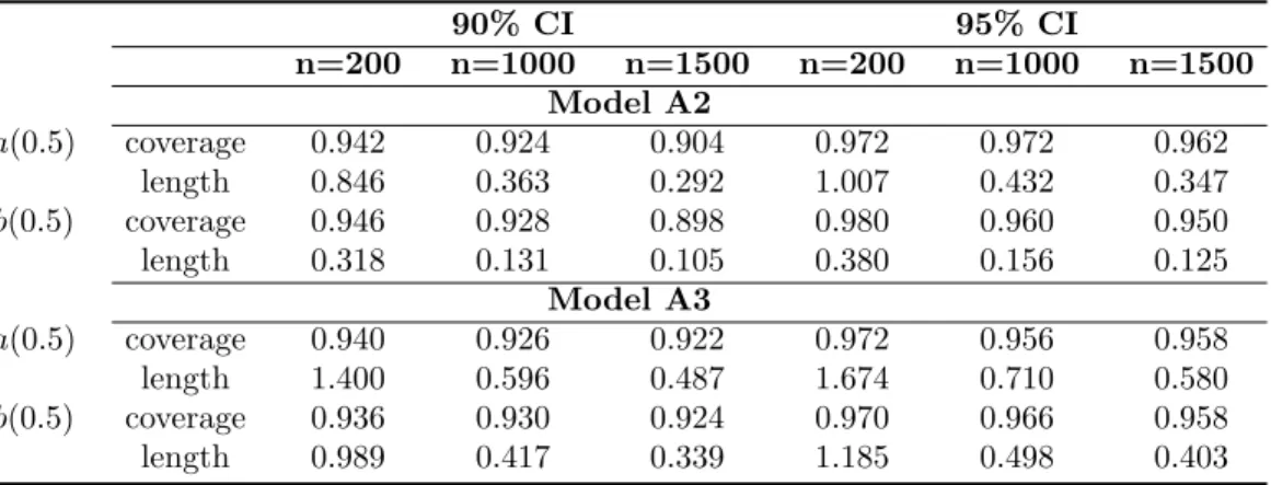
methods for Model A1: (1) BEL.s, (2) BTL based on the true likelihood, and (3) BDL based on a working Laplace likelihood. The coverage probability and lengths of the posterior intervals are computed over 1000 data sets of sample sizesn= 100,400,and 1600. . . 48 5.2 Coverage properties of BEL.s based on Models A2 and A3 . . . 48 5.3 Coverage properties of 95% CI with various priors for BEL.s in Models A2 and A3 . 49 5.4 The table presents the coverage probabilities and lengths of the posterior intervals
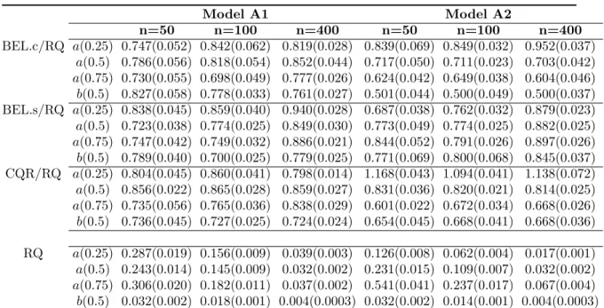
obtained from BEL.c for Models A1 and A2 . . . 52 5.5 The table presents the MSE ratios of BEL.c, BEL.s and CQR estimates over RQ
estimates for Models A1 and A2, respectively. The MSE of RQ estimates are listed in the bottom part the table. . . 53 5.6 The table presents the performance of the BEL estimates using different priors. For
BEL.p1 and BEL.p2, different values ofσare considered. . . 56 5.7 MSE Table based on Models A1, A2, A5, A4 and A6 with sample size 100 . . . 59 5.8 The table gives then×M SE0sof several estimators for the adjusted intercepts and
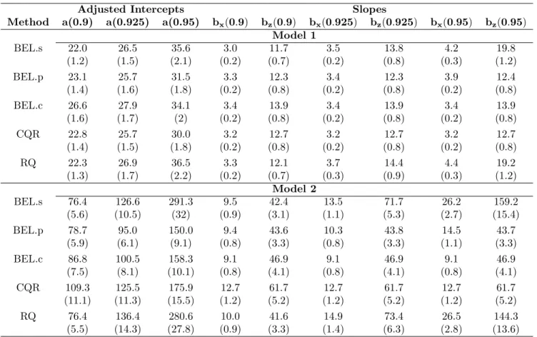
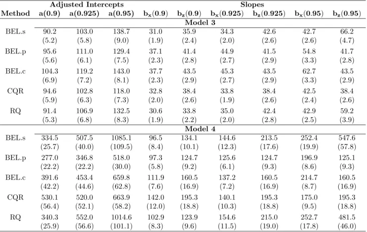
slope parameters at three quantile levelsτ = 0.9,0.925,0.95 for Models B1 and B2, where n= 100, and the M SE is averaged over 500 samples from each model. The numbers in the brackets are the estimated standard errors. . . 62 5.9 Simulation results for Models B3 and B4; see the caption of Table 5.8 for more details. 63 5.10 The MSE Table of BEL.s, BEL.m and RQ estimates at τ = 1/3 and 2/3 for sample
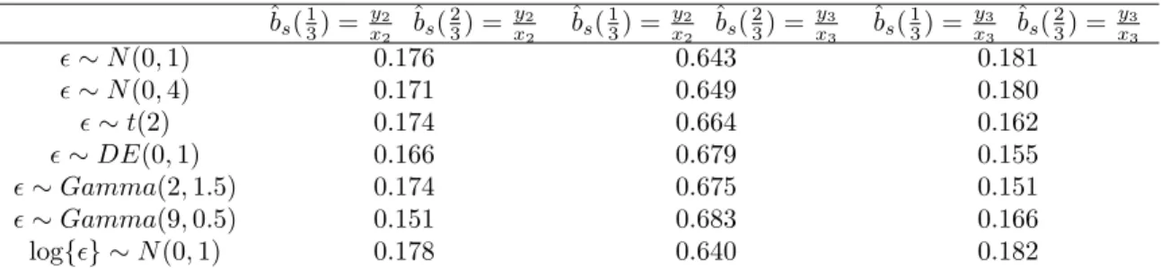
sizen= 4. The numbers in brackets are the standard error of the corresponding MSE. 68 5.11 The table presents the proportions of the BEL.s estimates among the cases of ˆbs(1/3) =
ˆbs(2/3) =y2/x2, ˆbs(1/3) =y2/x2,ˆbs(2/3) =y3/x3, and ˆbs(1/3) = ˆbs(2/3) =y3/x3. . 68 6.1 The table presents the normalized differences calculated by (6.2). The row names
provide the method used for model fitting. In the column names, the Whole Period indicates all the data in the testing period are used; Lower RTEM indicates the testing data with RTEM below its median; Wet Days indicates the testing data with RAIN equals to 1. . . 72 6.2 The table represents the mean absolute difference between the τ-th quantile
pre-dictions from downscaling and the fitted regression quantiles on the testing data at
Chapter 1
Introduction and Review
1.1
Introduction to quantile regression
Quantile regression is gradually developing into a systematic methodology for estimation of condi-tional quantile functions. Instead of focusing on the condicondi-tional mean based on the least squares regression, quantile regression could provide more comprehensive information on how the covariates influence the entire distribution of the response variables. Quantile regression is widely recognized for its superior properties, including robustness and the distribution-free property. Moreover, the modern linear programming techniques make the computation of quantile regression very efficient.
Koenker and Bassett (1978) specify the τ-th conditional quantile function as
Qτ(Y|X) =X>β(τ), (1.1)
which assumes that theτ-th quantile of the responseydepends linearly on the covariatesXwithout specifying the relations of the linear coefficients β(τ) acrossτ. The infinite dimensional β(τ) over
τ ∈(0,1) makes quantile regression essentially a nonparametric approach. The whole set {β(τ) :
0 < τ <1} describes the entire distribution of the response Y given the covariatesX. Motivated
by the finding of theτ-th sample quantile through
minξ∈R
n
X
i=1
ρτ(Yi−ξ), (1.2)
whereρτ(µ) =µ(τ−1{µ<0}), we estimateβ(τ) by ˆβn(τ), which solves
minβ∈Rp
n
X
i=1
ρτ(Yi−Xi>β). (1.3)
As discussed in Koenker (2005), ˆβn(τ), which are often called asregression quantiles, can be
can be explained as follows: in the finding of some particular sample quantile, every observation plays the role of order statistics and constitutes extreme points of the linear constraint set in the terminology of linear programming. Similarly, in solving for regression quantiles, points (x, y) play the role of order statistics and act as extreme points of the polyhedral constraint set. If we perturb the order statistics above (or below) some quantile in a way that they remain above (or below) the quantile, the position of that quantile is unchanged. Therefore, quantile regression preserves an important robustness property of the ordinary sample quantiles.
In regression, we often use two types of linear models:
Yi=Xi>β+ei, (1.4)
and
Yi=Xi>β+ (Xi>γ)ei, (1.5)
where the ei’s are i.i.d from distribution Fe, andXi includes the intercept. Model (1.4) is often
called a homoscedastic model, and Model (1.5) is a special heteroscedastic model, often called the linear location-scale model. For both Models (1.4) and (1.5), we can easily derive the corresponding implied relations ofβ(τ) defined in (1.1). In Model (1.4),
β(τ) = (Fe−1(τ), βs).
whereβs is the slope coefficient in (1.1). Clearly, in Model (1.4), the slope coefficients are the same
acrossτ. In Model (1.5),
β(τ) =β+γFe−1(τ).
Clearly,β(τ) vary withτ for non-zeroγ.
1.2
Review on inference for quantile regression
Through the discussion in Section 1.1, we see that Model (1.1) in quantile regression includes some common statistical models. By linear programming techniques, we can efficiently solve for ˆβn(τ).
In this section, we will review the approaches to inference for quantile regression.
Bassett (1978) give the finite-sample density of the regression quantile estimator ˆβn(τ) under the
i.i.d error distribution assumption. However, due to the high computational burden, the finite-sample density is formidable to be used in inference. As for the least squares estimation, we often rely on the asymptotic approximations of the distribution of ˆβn(τ). Koenker and Bassett (1978)
give the joint asymptotic distribution of the regression quantiles ˆζn = ( ˆβn(τ1)>, ...,βˆn(τm)>)> under
i.i.d errors, taking the form as: √ n( ˆζn−ζ) = √ n βˆn(τj)−β(τj) m j=1 d →N(0,Ω⊗Q−01), (1.6)
as n → ∞, where Ω is an m×m matrix with (ωij) = (τi∧τj−τiτj)/f(F−1(τi))f(F−1(τj)),Q0
is the limit ofn−1P
xix>i . This asymptotic result affords the scope for the Wald-type inference in
quantile regression. In the non-i.i.derror settings, the estimate ˆβn(τ) also has the asymptotic normal
property taking a more complicated form. One application of the asymptotic normality result is testing the equality of slope parameters across quantiles, which is considered in Koenker and Bassett (1982b). However, the utilization of the asymptotic results requires estimating the sparsity function evaluated at the quantile of interest, i.e.,{f(F−1(τ))}−1. Estimating {f(F−1(τ))}−1 is essentially
a smoothing problem, which is difficult when the observations around the quantile are sparse. Another approach of inference in quantile regression is rank-based. The Wilcoxon (1945) test for the univariate sample is well known for its better asymptotic relative efficiency to thet-test in a wide range of non-Gaussian error models. Besides, the Wilcoxon test statistic and its limiting behavior are independent of the data generating distribution F under the null hypothesis of no difference between two populations. The generalized rank test based on regression rank scores, proposed in Gutenbrunner and Jureˇckov´a (1992) inherits these properties, as discussed in Koenker (1996). The confidence intervals constructed based on regression rank scores do not need to be symmetric and can be better suited to the skewness of the data. Meanwhile, they enjoy the scale invariance of the test statistics and circumvent the problem of sparsity function estimation. However, the rank-based method is computationally expensive with respect to the calculation of confidence regions, and practically feasible for only one dimensional parameter at a time. Besides, it is still unclear how to estimate the variance covariance matrix for the estimated ˆβn(τ) by the rank-score method.
As an analog to the likelihood ratio tests, we can consider a quantile likelihood ratio test, as shown in Koenker and Bassett (1982b). The quantile likelihood ratio test borrows likelihood from the Laplace density. To work in non-i.i.d error settings, the termsρτ(Yi−Xi>b) in the objective
function need to be properly weighted to achieve the limitingχ2distribution for the test statistics. In Koenker and Portnoy (1987), a uniform, Bahadur type asymptotic representation of regression quantiles is established. In Portnoy and Koenker (1989) further propose a fully adaptive L-estimator for the slope parameter of a linear model. The estimator achieves substantial efficiency gain in a wide variety of error settings. However, the estimator is restricted to homoscadestic errors situation and depends on an efficient density estimation, which is non-trivial in practice.
The bootstrap and other sampling schemes can be used for inference in quantile regression. Efron (1982) suggests bootstrapping the residuals for a nonlinear median regression problem. De Angelis and Young (1993) further show that sampling residuals from a smoothed version of its distribution instead of its empirical distribution will reduce the bootstrap approximation error fromO(n−1/4) to
O(n−2/5). However, resampling residuals cannot be applied to non-i.i.d error settings. The (x, y) paired bootstrap provides a simple and effective alternative for independent but not identically dis-tributed error settings. Similar to bootstrapping residuals, there are also several proposals for paired bootstrap through smoothing. Horowitz (1992) proposes smoothing the quantile regression objec-tive function to gain refinements in the asymptotic accuracy of rejection probabilities based on the bootstrap critical values in the Wald-type tests. This method needs estimation of the sparsity and requires selection of a bandwidth in smoothing the objective function, although it is demonstrated through simulations in Horowitz (1992) that the results are not very sensitive to bandwidth choices. Although paired bootstrap is reliable, it is time consuming for large data sets. Kocherginsky et al. (2005) propose a Markov chain marginal bootstrap (MCMB) method to construct confidence in-tervals for quantile regression. The MCMB method also avoids the estimation of the error density. Compared to the paired bootstrap and the rank score test, the MCMB method is more practically feasible to handle high dimensional parameters and large data sets. Another option for refinements of the paired bootstrap is subsampling. The results in Buchinsky (1995) suggest that subsampling in bootstrap can produce more accurate confidence levels than the usual bootstrap. The subsampling technique has two advantages: first, it saves computational cost, especially when the sample size is very large; second, it works like smoothing the empirical distribution function. Some data-driven rules for choosing the subsampling size are suggested in Bickel and Sakov (2008).
1.3
Introduction to empirical likelihood
Likelihood methods are often used to find efficient estimators, and to construct tests with good power properties. A problem with parametric likelihood methods is that we might not know which parametric family to use. Model misspecification can cause likelihood-based methods to be biased or inefficient. Nonparametric inferences are therefore preferred when we want to avoid the specification of a parametric family for the data.
The name empirical likelihood is used because the empirical distribution of the data plays a central role in the methodology. Before the introduction of empirical likelihood, we first review two concepts as in Owen (2001): the empirical cumulative distribution function and the nonparametric likelihood. Let X1, X2, ..., Xn be an independent random sample from some common distribution
functionF0. The empirical cumulative distribution function (ECDF) ofX1, X2, ..., Xn is defined as
Fn(x) = 1 n n X i=1 1{Xi≤x}, (1.7)
where 1{X≤x} is the indicator function of the set {X ≤x}. Given X1, X2, ..., Xn ∈ Ras an
inde-pendent random sample from some common distribution functionF0, the nonparametric likelihood
of the CDFF is L(F) = n Y i=1 (F(Xi)−F(Xi−)). (1.8)
It is first noticed by Kiefer and Wolfowitz (1956) that ECDF is a nonparametric maximum likelihood estimate. Following the idea of basing tests of hypothesis and confidence regions on the likelihood ratio as in parametric inference, we may also use ratios of the nonparametric likelihood to perform hypothesis testing and confidence intervals. The earliest known use of empirical likelihood ratio functions is in Thomas and Grunkemeier (1975) for constructing confidence intervals for the survival function based on censored data. For a distribution F, R(F) = L(F)/L(Fn) is defined as the
nonparametric likelihood ratio, whereFnis the ECDF. Suppose that we are interested in a parameter
θ that satisfies Em(X, θ) = 0 for some estimating function m(X, θ), the profile likelihood ratio function is defined as:
R(θ) = sup
R(F)EFm(X, θ) = 0, F ∈ F ,
whereFis some pre-specified set of distribution functions onR. Similar to the parametric likelihood ratio test, the empirical likelihood ratio test rejects the hypothesis θ =θ0 when R(θ0) is smaller
regions is straightforward. However, to make the methodology feasible in practice, we need to clarify the domain ofF and the choice of r0. As presented in Owen (2001), F could be further narrowed
down to the discrete distribution functions that assign weights to the observationsXis. Therefore,
the profile empirical likelihood ratio function can be reformulated as
R(θ) = maxn n Y i=1 nωi n X i=1 ωim(Xi, θ) = 0, ωi≥0, n X i=1 ωi= 1 o .
The above reformulation makes the calculation ofR(θ) feasible for any givenθ. We defer the detailed discussion on the computation ofR(θ) to Chapter 2.
The remaining issue is how to decide the threshold valuer0. Owen (1988) provides the univariate
empirical likelihood theorem (ELT), which shows that−2 logR(µ0) has a limiting distribution of the
chi-square distribution with 1 degree of freedom under the null hypothesisθ=µ0. Noticing that the
chi-square limit is also what we typically find for the parametric likelihood ratio test with only one parameter, this univariate ELT is often viewed as a nonparametric analogue of the Wilk’s theorem, which is first proposed in Wilks (1938). Owen (1990, 1991) extend the conclusion in the univariate ELT to statistics that can be written as smooth functions of means or that are defined through estimating equations. The above ELT theorems can also be used to construct confidence regions for the parameters of interest. Owen (1988) shows that the coverage error of the two-sided confidence intervals based on ELT is O(n−1), which is typically true for the coverage error in parametric likelihood intervals. Moreover, it has been observed that the true coverage of the confidence interval by ELT is usually below the nominal level for finite samples.
Another important issue is the power and efficiency of the empirical likelihood inference. Lazar and Mykland (1998) compare the asymptotic power of the empirical likelihood and the parametric likelihood, and show that the power of the empirical likelihood based tests matches that of the parametric likelihood to the second order, if the empirical likelihood uses the same likelihood-based estimating equation. The third order properties of the power expansion of empirical likelihood tests could be better or poorer than the parametric likelihood tests. Moreover, it is well known that a Barlett correction can be used to reduce the coverage errors of the two-sided confidence intervals based on parametric likelihoods from O(n−1) toO(n−2), as shown in DiCiccio et al. (1991) based on Hall and La Scala (1990). DiCiccio et al. (1991) show that the empirical likelihood inference for smooth function of means is also Barlett correctable. Zhang (1996) shows that the Barlett correction for the univariate mean can be applied for univariate parameters defined through one dimensional
estimating equations.
In the parametric likelihood inference, we know that the maximum likelihood estimator ˆθM LE
en-joys some nice properties. For example,−2 logL(ˆθM LE) has a chi-square limiting distribution under
the assumption that the likelihood is correct. Qin and Lawless (1994) explore the analogous prop-erties for the maximum empirical likelihood estimator (MELE). They show that−2 logR(ˆθM ELE)
has the chi-square limiting distribution, and that the MELE estimator is asymptotically efficient in the sense that it has the same asymptotic variance as the optimal estimator obtained from the class of estimating equations as linear combinations of the moment constraints used in the empirical likelihood inference.
The empirical likelihood methods inherit many of the same asymptotic properties as those from the parametric likelihood. The combination of the flexibility of the nonparametric methods and the reliability and effectiveness of the likelihood approach makes the empirical likelihood methods appealing options in nonparametric inferences. The empirical likelihood methods have been applied to various statistical models, like partial linear models in Yang et al. (2009) and Liang et al. (2009), longitudinal data in You et al. (2006) and Wang et al. (2010), and heteroscedastic accelerated failure time model in Zhou et al. (2011).
1.4
Empirical likelihood for quantiles
Empirical likelihood methods can be used to estimate quantiles. Generally for 0< τ <1, theτ-th quantileQτ of some distributionF is the solution of
E 1{X≤Qτ}−τ
= 0.
GivenX1, X2, ..., Xn ∈ Ras an independent random sample from some common distribution
func-tionF0, for X(1)< q < X(n)and 0< p <1, letZi(p, q) = 1Xi≤q−p. Then we have the empirical
likelihood ratio defined as
R(p, q) = maxn n Y i=1 nωi n X i=1 wiZi(p, q) = 0, ωi≥0, n X i=1 ωi = 1 o . (1.9)
Unlike the empirical likelihood ratio of sample mean, which has no analytical expression, (1.9) has a simple analytic form:
where ˆp= ˆp(q) =]{Xi≤q}/n, i.e. the proportion of samples that are smaller or equal thanq. By
the ELT theorem of Owen (1991), −2 logR(p, q) has the limiting distribution χ2(1); and thus we
can construct confidence intervals forQτ. However, because of the non-smoothness ofZi(p, q) as a
function ofq, the coverage error of the confidence intervals forQτ is of orderO(n−1/2) rather than
O(n−1).
In the literature, some research has been aimed at reducing the coverage error of the confidence intervals for Qτ. Noticing that the reason for the low error rate O(n−1/2) is the involvement of
the indicator function 1{Xi≤q}, Chen and Hall (1993) introduce a kernel smoothing technique to
smooth 1{Xi≤q} first and then construct the confidence regions from empirical likelihood based on
the smoothed estimating equations. The coverage error can be reduced toO(n−1) by smoothing, and further toO(n−2) by Barlett correction. Like other kernel smoothing problems, there also arise issues on the choices of the bandwidth h to achieve the coverage error of O(n−1) size. Chen and
Hall (1993) show that to achieve the coverage error of O(n−1), the bandwidth hneeds to satisfy
conditions thath=o(n−1/2) and nh/log(n)→ ∞; to achieve the coverage error of almostO(n−2)
under the Barlett correction, hhas to satisfy conditions that h=O(n−3/4) and nh/log(n)→ ∞.
These theoretical results provide some idea about the choices ofh, however,they provide a range for
h, which is too vague to offer good practical guidance. There is no optimal choice ofhprovided in the literature, although it is indicated through simulation studies that the coverage error could be reduced by many reasonable choices ofh.
The empirical likelihood methods can also be used to estimate parameters β(τ) in the quantile regression models (1.1) and construct the confidence regions for these parameters. Motivated by the subgradient condition in quantile regression, the estimates of the regression quantilesβ(τ) satisfies an estimating equation with
m(Y, X, β(τ)) = 1{Y≤X>β(τ)}−τX. (1.10)
Whang (2006) extends the idea of Chen and Hall (1993) to use the kernel smoothing technique on the indicator function 1{Y≤X>β(τ)}in (1.10), and therefore achieves some higher order properties of
O(n−1) and evenO(n−2) after Barlett correction. Similar to the empirical likelihood inference on univariate quantiles, the choices of the bandwidthh in the kernel smoothing have been suggested ambiguously.
conditional empirical likelihood by Kitamura et al. (2004). The conditional empirical likelihood calculates locally the empirical likelihood for every observation Xi by borrowing information from
the neighboring observations. The basic idea is to maximize some kernel weighted product of weights on the samples in a neighborhood ofXi under the moment restrictions:
E 1{Y≤X>β(τ)}−τ|X= 0, (1.11)
where the conditional expectation is approximated by smoothing overx. The relationship between the conditional empirical likelihood and the empirical likelihood is analogous to that of the weighted quantile regression of Newey and Powell (1990) and the quantile regression of Koenker and Bassett (1978). From the computational viewpoint, the local empirical likelihood of every proposed β(τ) conditional on some Xi has an analytic expression, because conditioning on Xi, the estimating
equation in (1.11) is essentially the same as (1.9). However, the local empirical likelihood needs to be calculated for every Xi and the proposed analytical expression in Kitamura et al. (2004)
works only for univariate quantiles. Otsu (2008) further proposes some smoothed counterpart of the conditional empirical likelihood with quantile regression. By smoothing the indicator function 1{Y≤X>β(τ)} in (1.11), the smoothed conditional empirical likelihood method in Otsu (2008) allows
some standard Newton-type optimization algorithm to search for the maximum empirical likelihood estimate, although the Newton-type algorithm can not be guaranteed for convergence.
1.5
Empirical likelihood and some other nonparametric
inference approaches
Besides the empirical likelihood methods (EL), there are some other nonparametric inferential ap-proaches whose statistical models are also defined through moment restrictions. They include the two-step efficient generalized methods of moments (GMM) estimator of Hansen (1982), and the exponential tilting (ET) estimator of Kitamura and Stutzer (1997). As shown in Smith (1997), EL and ET share some common structures, belonging to the family of generalized empirical likelihood (GEL) estimators. All of these estimators (GMM, EL and ET) share the same asymptotic distri-butions but differ in higher order asymptotic properties. Newey and Smith (2004) conclude that EL has two theoretical advantages: first, compared to GMM, the (asymptotic) bias of EL does not grow with the number of moment restrictions; Second, after bias correction, the EL is higher order
efficient compared to other bias corrected estimators.
Among the GEL estimators, EL and ET are two important members. Both of them can be inter-preted as the minimum empirical discrepancy (MED) estimators, as in Cressie and Read (1984),Cor-coran (1998): ˆ θ= argminθ∈Θn−1 n X i=1 h(ˆωi(θ)) ,
where ˆωi(θ) is the solution to
min{ωi,1≤i≤n}n −1 n X i=1 h(ωi),
subject to the moment and normalization constraints:
n X i=1 ωim(xi, θ) = 0, n X i=1 ωi= 1.
The discrepancy is h(ω) =−log(nω) used in EL and h(ω) =nωlog(nω) in ET. Clearly, EL is to maximize a quantity analogous to the likelihood, while ET is to maximize an entropy-like quantity. It has been shown that the MELE and METE, the estimator maximizing EL and ET, respectively, are asymptotically equivalent to the first order. However, Baggerly (1998) shows that EL is the only one among the MED estimators that allows a Barlett correction. As shown in Smith (1997), EL enjoys higher-order asymptotic properties than ET and GMM when the model is correctly specified. Schennach (2007) shows that when the model is misspecified, i.e., the moment restrictions are misspecified, the asymptotic variance of MELE may become undefined if the functions defining the the moment conditions are unbounded, but METE can avoid such problem under some regularity conditions. Schennach (2007) further introduces a new estimator based on the exponentially tilted empirical likelihood (ETEL), which is some combination of EL and ET. The ETEL estimator has been shown to enjoy the same higher order properties as EL, and maintain a well-defined asymptotic variance when the model is misspecified.
The bootstrap is also a widely used nonparametric inference approach. Compared to empirical likelihood, bootstrap methods enjoy smaller computational cost . However, as pointed out in Owen (2001):
The main advantage of empirical likelihood, relative to bootstrap, stems from its use of a likelihood
function. Not only does empirical likelihood provide data-determined shapes for confidence regions, it
can also easily incorporate known constraints on parameters, and adjust for biased sampling schemes.
Unlike the bootstrap, empirical likelihood can be Barlett corrected, improving the accuracy of
infer-ence. Likelihoods also make it easier to combine data from multiple sources, with possibly different
sampling schemes.
Despite the differences discussed above, it is worth noting that these nonparametric inference approaches can be combined effectively to further improve the estimation efficiency or reduce the error in hypothesis testing based on only one approach. Bootstrap methods are often used to decide the critical value in hypothesis testing based on EL, ET or GMM. Besides, the implied weights in EL or ET can also be used as the resampling probabilities in bootstrap. One example to illustrate the cooperation of GMM, bootstrap and EL can be found in in Brown and Newey (2002), which proposes a novel method of bootstrapping for GMM by resampling from the empirical likelihood distribution to improve the asymptotic approximation for GMM in finite samples.
1.6
Bayesian empirical likelihood for quantile regression
(BEL)
Although there is already intensive development of quantile regression in various areas, see Koenker (2005), there is still room for improvement. Theτ-specific models in (1.1) allow for great flexibility, asβ(τ) for upper or lower quantiles can be distinct from central trends, but the quantile estimates are highly variable in data-sparse areas. Taking advantage of some commonality across quantile coefficientsβ(τ) acrossτ can provide a desirable balance in the bias-variance tradeoff. In our work, we consider using prior information onβ(τ) across severalτ values. For example, a common slope assumption for τ near 1 can improve the efficiency of high quantile estimation. Other forms of informative priors on β(τ) may achieve a similar goal. Bayesian methods are a natural way of combining data with prior information. The main difficulty to put the Bayesian method to work for quantile regression is that the model onQτ(Y|X) for one or moreτ values does not specify a
parametric likelihood, which is needed in the Bayesian framework.
In our work, we focus on the empirical likelihood (EL), introduced by Owen (1988), to incorporate quantile regression into a Bayesian framework. We begin with notations and definitions of the underlying models and moment restrictions. Let D = {(Xi, Yi), i = 1, ..., n} be a random sample
from the following quantile regression model
Qτ(Y|X) =X>β0(τ), (1.12)
whereX ∈Rp+1is composed of an intercept term andpcovariates. We assume that the distribution
of thepcovariates,GX, has a bounded supportχ. If the design points are non-stochastic, the basic
conclusions we obtain in our work hold under appropriate conditions on the design sequence, but we focus on the case of random designs for simplicity. The unknown functionβ0(τ), if specified over all
τ∈(0,1), describes the entire conditional distribution ofY givenX, which is denoted asFX in the
rest of the thesis. We consider the problem of estimatingkquantiles atτ1< τ2< ... < τk, and let
ζ0= (β0(τ1), ..., β0(τk)) be the true parameter of interest inRk(p+1). To estimateζ0, we usek(p+ 1)
dimensional estimating functionsm(X, Y, ζ), whereζ= (β(τ1), ..., β(τk)) and the components ofm
are mdk+j(X, Y, ζ) =ψτd+1 Y −X >β(τ d+1)Xj, (1.13) ford= 0,1, ..., k−1,j= 0,1, ..., p, with ψτ(u) = n 1{u<0}−τ u6= 0 0 u= 0
being the quantile score function.
For any proposedζ, its profile empirical likelihood ratio is given by
R(ζ) = maxn n Y i=1 (nωi) n X i=1 ωim(Xi, Yi, ζ) = 0, ωi≥0, n X i=1 ωi= 1 o . (1.14)
With a prior specificationp0(ζ) on the parameterζ, we can formally have the posterior density
p ζ|D
∝p0(ζ)× R(ζ). (1.15)
We callp ζ|D
the posterior distribution from the BEL approach. This can be viewed as a misnomer, chosen for the sake of convenience, because it is not really a posterior in the strict sense. Lazar (2003) proposed a procedure to check whether the empirical likelihood is valid for posterior inference based on the criteria provided in Monahan and Boos (1992). In this paper, we focus on the asymptotic
properties of the posterior distribution (1.15), and establish its frequentist validity by first-order asymptotics.
Clearly, the empirical likelihood framework allows the joint estimation of multiple quantiles. By using the common parameters inζ over differentτ, we calculate the empirical likelihood with more moment equations than the number of parameters. For example, if we believe the model is homoscedastic, we will takeβs(τ1) =βs(τ2) =...=βs(τk), whereβs(τ) denotes theβ(τ) excluding
the intercept. Moreover, we can assumeβs(τ) =βs(τ0) +r(τ−τ0) for some preassumedτ0, which
indicates the slope parameters βs(τ) linearly vary over τ. By doing so, we actually reduce the
dimensionality of the parametersβ(τ). As shown in Qin and Lawless (1994) for smooth estimating functions, the maximum empirical likelihood estimator attains the optimal asymptotic efficiency subject to those moment conditions. We expect the same for quantile estimating functions.
Compared to the EL esimator, our proposed BEL approach has its own merits in applications where informative priors onβ(τ) might be more appropriate than strict functional relationship on some of the parameters. For example, we may believe that the slopes β(τ1) are roughly the same
asβ(τ2). Imposing strict equality to reduce the number of unknown parameters inζmight be hard
to justify, but an informative prior on the difference of the two neighboringβ(τ) can help regulate quantile estimation.
Besides the fact that an informative prior might help improve the estimation efficiency, the Bayesian empirical likelihood method also helps the search of the maximum empirical likelihood estimates by using nearly flat priors. The optimization of empirical likelihood over high dimensional parameters is usually painful. Instead of directly maximizing the empirical likelihood over β(τ), a Bayesian computation algorithm can make the search more effective.
The challenges of the Bayesian empirical likelihood for quantile regression come in two forms. First, the empirical likelihood itself is computationally expensive. Therefore, an efficient algorithms to solve for empirical likelihood at a particular β(τ) is needed to make the Bayesian computation feasible. The computational issue will be discussed in more detail in Chapter 2. Second, the existing work on the theoretical properties about empirical likelihood is mainly for smooth moment restrictions and therefore cannot be evoked for the quantile regression settings directly due to the involvement of the indicator function in (1.10). The work in Lazar (2003) is chiefly based on smooth estimating equations, especially for the mean case. Lazar (2003) also provides mostly heuristic arguments for the asymptotic properties of the resultant posterior quantities. The lack of smoothness in the quantile based moment restrictions does not allow Taylor expansion, and thus we need to use
the empirical process theory to show the theoretical properties of the posterior quantities produced by the Bayesian empirical likelihood for quantile regression.
The empirical likelihood is not a likelihood in the usual sense, so the validity of the resultant pos-terior does not follow from the Bayes formula. Lazar (2003) discussed the validity of inference for the Bayesian empirical likelihood (BEL) approach based on earlier work of Monahan and Boos (1992). Schennach (2005) and Lancaster and Jun (2010) considered Bayesian exponentially tilted empirical likelihood (ETEL), which can be viewed as a nonparametric Bayesian procedure with noninforma-tive priors on the space of distributions. Lancaster and Jun (2010) further considered Bayesian ETEL in quantile regression. For the inference of population means, Fang and Mukerjee (2006) investigated the asymptotic validity and accuracy of the Bayesian credible regions, and furthermore, Chang and Mukerjee (2008) showed that EL admits posterior based inference with the frequentist asymptotic validity, but many of its variants do not enjoy this property. To establish the asymptotic validity of the BEL for quantile regression, we need to work with the quantile estimating equations that involve discontinuous functions, so direct local expansions used in the EL literature cannot be used. Chernozhukov and Hong (2003) discuss on the asymptotic properties of the quasi-posterior distributions defined as transformations of general (nonlikelihood-based) statistical criterion func-tions, including empirical likelihood. In our work, we also establish the asymptotic distributions of the posterior from the BEL approach for quantile regression. Different from Chernozhukov and Hong (2003), we are particularly interested in the interaction of informative priors and empirical likelihood on the asymptotic distribution of the posterior, which enables us to evaluate efficiency gains from informative priors. Although finite-sample validity of the BEL posterior inference cannot be expected in our setting, we continue to use the term “posterior” throughout the article.
In the literature of quantile regression, there are some valuable attempts to estimate multiple quantiles jointly. Zou and Yuan (2008) propose a new quantile regression methodcomposite quantile regression(CQR) to estimate multiple quantiles jointly. Because the CQR method is developed to improve the estimation efficiency over the least squares in model selection, it is constructed under thei.i.d error assumption with common slopes across different quantiles. Thus, the CQR has only one slope parameter for all the quantiles considered, and the estimation efficiency of that common slope parameter takes the form of a combination of individual quantile regression estimates. This combination may obtain higher efficiency at some quantiles, usually the more extreme quantiles, while sacrificing efficiency at some other quantiles, usually quantiles near the median. Additionally, the CQR combines the objective functions of different quantiles by assigning equal weights to each
quantile. Other choices of weights may result in more efficient estimators. Koenker (1984) considers a more general case when unequal weights are allowed. The Bayesian empirical likelihood for quantile regression avoids the choice of weights on different quantiles. As shown in Qin and Lawless (1994), the empirical likelihood method combines information from the estimating equations in an optimal way, which indicates that the Bayesian empirical likelihood method would automatically pick up the optimal weights in combining the estimation equations for different quantiles.
The development of generalized method of moments (GMM) provides another option to esti-mate multiple quantiles jointly. Hansen (1982) constructs a comprehensive framework for GMM and develops the asymptotic theorys for the GMM estimator. The GMM estimators, the maximum empirical likelihood estimator (MELE), and some other EL-type estimators generally have the same asymptotic distributions, but possibly different higher order asymptotic properties, see Newey and Smith (2004) and Schennach (2007). As discussed in Newey and Smith (2004), the empirical like-lihood approach has advantages over the GMM estimators. Unlike GMM, the (asymptotic) bias of the MELE does not grow with the number of moment restrictions. Furthermore, the efficiency of the GMM estimator relies on a covariance matrix estimate for the estimating equations, which could be ill-conditioned in the problem of estimating multiple quantiles. Yin (2009) proposes a Bayesian version of GMM, taking the exponential form of the negative weighted GMM quadratic objective function divided by two as the working likelihood in Bayesian inference. Bayesian GMM is able to account for the underlying correlation among the data by using a correlation matrix in estimation. Actually Bayesian GMM has similarities with Bayesian empirical likelihood methods. They both avoid the full parametric likelihood formulations of the data and only require moment conditions. By taking advantage of the Bayesian computation, both methods circumvent the numerical opti-mization difficulties in GMM and in the maximum empirical likelihood estimation. However, both Bayesian GMM and Bayesian empirical likelihood methods lack an exact Bayesian interpretation in finite samples, so large-sample properties need to be studied.
In our work, we develop the Bayesian empirical likelihood method for quantile regression. We use a modified Newton-Raphson type algorithm to efficiently calculate empirical likelihood, and establish the theoretical properties of the resultant posterior quantities. In simulation studies, we apply the method to different settings with various priors, to see how well the Bayesian empirical likelihood method compares with some standard approaches when informative priors are used. We show that significant efficiency gains can be expected by making use of common features across
approach can be used as a useful statistical downscaling method for the projection of high quantiles of temperatures from large scale climate models to a local scale. As a future extension, we extend the BEL approach in spatially correlated data.
Chapter 2
Computation
In this chapter, we discuss on the computational issues of the BEL approach. In our BEL ap-proach, we employ empirical likelihood as a working likelihood for quantile regression. With a prior specification p0(ζ) on the parameter ζ, we can formally have the posterior density (1.15). Using
(1.15), we can calculate the empirical likelihood value up to some normalizing constant. Therefore, the Metropolis-Hastings algorithm, as given in Hastings (1970), is feasible for sampling from the posterior.
This chapter is organized as follows. In Section 2.1, we will describe an efficient modified Newton-Raphson algorithm to calculate the empirical likelihood value for a givenζ. In Section 2.2, we will discuss on the utilization of the Metroplis-Hasting algorithm in the Bayesian computation.
2.1
The modified Newton-Raphson algorithm for
calculation of empirical likelihood
By using the Metroplis-Hasting algorithm, in every step when we propose a new value forζ. its em-pirical likelihood value has to be evaluated. Therefore, an efficienct algorithm to calculate emem-pirical likelihood value for a givenζ is critical in the computation. In this section, we will describe how to use a modified Newton-Raphson algorithm to calculate the empirical likelihood efficiently.
For any proposedζ, its profile empirical likelihood ratio is given by
R(ζ) = maxn n Y i=1 (nωi) n X i=1 ωim(Xi, Yi, ζ) = 0, ωi≥0, n X i=1 ωi= 1 o .
Assuming 0 is in the convex hull ofm(Xi, Yi, ζ), then by the usual Lagrange multiplier method as
has the following solution R(ζ) = n Y i=1 nωi, whereωi= 1 n 1 1 +λ>m(X i, Yi, ζ) .
Under the condition that the Hessian matrixHθ(λ) =P n i=1
m(Xi,Yi,ζ)m(Xi,Yi,ζ)>
(1+λ>m(X
i,Yi,ζ))2 is positive definite
over the convex set
D=λ: 1 +λ>m(Xi, Yi, ζ)>0,1≤i≤n ,
the multiplierλ=λ(ζ)∈Rk(p+1) exists and is uniquely determined by
g(λ, ζ) = n X i=1 m(Xi, Yi, ζ) 1 +λ>m(X i, Yi, ζ) = 0.
For general estimating functions m(X, Y, ζ), usually there is no analytical solution of λ to
g(λ, ζ) = 0, and therefore, there is no analytical expression of R(ζ) as a function of ζ. One ex-ception is m(X, ζ) = 1X≤ζ −τ. This analytical expression reduces the cost of calculating the
empirical likelihood estimate for theτ-th conditional quantile regression at eachτ ∈(0,1), see Otsu (2008). For estimating functions m(X, Y, ζ) with no analytical solution ofλ(ζ), a seemingly direct way is to solve for λ through g(λ, ζ) = 0 first and then get the corresponding R(ζ). Obviously, solving forλ(ζ) directly throughg(λ, ζ) = 0 might be computationally expensive. By Owen (1990), an alternative efficient way to solve forλ(ζ) is to maximize the concave function
˜ l(λ) = n X i=1 log(1 +λtm(Xi, Yi, ζ))
over the convex set D. Naturally, the unique solution of λ is expected to be found through some modified version of the Newton-Raphson algorithm efficiently. Chen et al. (2002) provide a modified Newton-Raphson algorithm to obtain range restricted weights for regression estimators for survey sampling, in which the estimating functionm(X, θ) =X−θ. Wu (2004) further discusses how to utilize this algorithm in non-stratified sampling and even stratified sampling with suitable formu-lations of the algorithm. Noticing that this algorithm is similar to the modified Newton’s method described in Polyak (1987), and some mild conditions are needed to guarantee the convergence of the optimization process. Chen et al. (2002) give a detailed discussion on those conditions and show they are satisfied when m(X, θ) = X −θ. Because these conditions are on the behavior of the objective function ˜l(λ), we could naturally extend this modified Newton-Raphson algorithm to the
general estimating functionm, regardless of the smoothness ofm(X, θ). In general,the corresponding constraints onm(Xi, θ) are:
M1 The vector 0k(p+1)∈Rk(p+1)is within the convex hull ofm(Xi, Yi, ζ),i= 1, ..., n.
M2 The matrixPn
i=1m(Xi, Yi, ζ)m(Xi, Yi, ζ)
> is positive definite.
The above two constraints could easily be satisfied for ζ near ζ0. Moreover, the condition M1
implies that the solution ofλexists forg(λ, ζ) = 0. When there is no solution for some proposedζ, it is reasonable to regard empirical likelihood atζas 0, which implies thatζis not within the feasible space of parameters. Under the above two constraints, the modified Newton-Raphson algorithm for generalm(X, ζ) listed below will find the optimalλmaximizing the objective function ˜l(λ):
Step 0: initialize λ0 = 0, k = 0, γ0 = 0, N = 500 as the maximum number of iterations and
= 10−8. The maximum iterationN andare used in the stopping rule.
Step 1: Calculate ∆(λ) ={ ∂ ∂λg(λ)} −1g(λ) = ( − n X i=1 m(Xi, Yi, ζ)m(Xi, Yiζ)> (1 +λ>m(X i, Yi, ζ))2 )−1 n X i=1 m(Xi, Yi, ζ) 1 +λ>m(X i, Yi, ζ) ,
Ifk∆(λk)k< εork > N, stop the algorithm and reportλk; otherwise go to step 2.
Step 2: Calculateδk =γk∆(λk). If 1 + (λk−δk)>m(Xi, Yi, ζ)≤0 for somei, or ˜l(λk−δk)<˜l(λk),
letγk =γk/2 and repeat Step 2.
Step 3: Setλk+1=λk−δk,k=k+ 1, andγk+1= (k+ 1)−1/2. Go to Step 1.
For the above modified Newton-Raphson algorithm, we make the followin remarks.
Remark 1: As mentioned in Wu (2004),Step 2ensures thatλis still within the convex setDand the objective function ˜l(λ) is moving towards its maximum point.
Remark 2: As suggested in Owen (1990), instead of making a preliminary check of whether 0 is within the convex hull ofm(Xi, Yi, ζ),1≤i≤n,which actually indicates whether the empirical
likelihood value exists for the proposedζ, we could do this check duringStep 1by checking whether 1 +λ>m(Xi, Yi, ζ) for 1 ≤i ≤ n. If 1 +λ>m(Xi, Yi, ζ) > 0 for all 1 ≤ i ≤ n, we will stop the
algorithm because the proposed ζ is not feasible or the corresponding ˜l(λ) = −∞. This revision makes the above algorithm more efficient.
Remark 3: When the dimension of the estimating functions is large, the stopping criteria of
= 10−8 and N = 500 may not be large enough to get sufficiently accurate empirical likelihood
calculated, especially forζnear the boundary.
Remark 4: The convergence theorem as in Chen et al. (2002) only ensures that the above algorithm performs well with infinite precision after infinitely many iterations. While in practice, we have to agree on finite approximations. That is why we use a stopping criterion with finite steps and small enough . From our limited experience, the algorithm encounters difficulty whenζ approaches the boundary. As mentioned in Owen (1990), a natural and reasonable goal for computation is that the algorithm is able to calculate log empirical likelihood ratio accurately enough for ζ within a confidence region with the coverage level well beyond what is expected in practice. Hence, we could either choose some properor the maximum number of iterationsN, or narrow the feasible region by excludingζ whoseλ(ζ) is too large, because largeλ(ζ) implies thatζ is near the boundary.
2.2
Bayesian Computation
The formulation of the posterior in (1.15) allows the utilization of the standard Metroplis-Hasting algorithm, as proposed in Hastings (1970), in the Bayesian computation. Assume using a normal distribution as the proposal distribution. The probability of moving fromζto ζ∗ is
α= min
1, R(ζ)×p0(ζ)
R(ζ∗)×p
0(ζ∗)
. (2.1)
We may use the average of the resultant Markov chain onζto be an estimate ofζ, when the posterior looks close to normal; otherwise, we suggest using the mode of the posterior, which maximizes (1.15). By choosing a proper prior, the posterior in (1.15) is proper. Therefore, by checking the detailed balance equation and Theorem 4.2 in Gilks et al. (1996), it is easy to show that the distribution of the MCMC sampler utilizing the moving probability in (2.1) converges to the posterior in (1.15). Similarly as the results provided in Chernozhukov and Hong (2003), the BEL estimates are as efficient as the extremum estimates. Moreover, the inference procedures based on the quantiles of the resultant posterior distribution produce asymptotically valid confidence intervals, which will be shown in Chapter 4.
In practice, we can always choose the initial value of the Markov chain as the usual quantile regression estimates. The Markov chain from the BEL usually approaches to its limit fast enough for moderate problems, i.e. problems with enough data around the quantiles of interest. However, we need to be more careful when we are interested in quantiles at tails, especially when multiple quantiles are jointly estimated. Usually a preliminary chain is needed to choose a proper proposal
distribution. A long enough burning period and a longer chain are also needed to gurranttee the chain has mixed.
Finding the maximum empirical likelihood estimator is a daunting task computationally, because the objective function is generally multi-modal. When the prior densityp0(ζ) is nearly flat, our BEL
approach employing the Metroplis-Hasting algorithm can be viewed as an alternative way to search for the maximum empirical likelihood estimator. Besides, our results in Chapter 4 suggests that the resultant posterior chain is valid for inference in the frequentist sense.
Chapter 3
Properties of the Maximum
Empirical Likelihood Estimate
(MELE)
3.1
Introduction
LetD={(Xi, Yi), i= 1, ..., n}be a random sample from the following quantile regression model
Qτ(Y|X) =X>β0(τ), (3.1)
whereX ∈Rp+1is composed of an intercept term andpcovariates. We assume that the distribution
of thepcovariates,GX, has a bounded supportX. If the design points are non-stochastic, the basic
conclusions we obtain in this paper hold under appropriate conditions on the design sequence, but we focus on the case of random designs for simplicity. The unknown functionβ0(τ), if specified over
allτ∈(0,1), describes the entire conditional distribution ofY givenX, which is denoted asFX in
the rest of the thesis. We consider the problem of estimatingkquantiles atτ1< τ2< ... < τk, and let
ζ0= (β0(τ1), ..., β0(τk)) be the true parameter of interest inRk(p+1). To estimateζ0, we usek(p+ 1)
dimensional estimating functionsm(X, Y, ζ), whereζ= (β(τ1), ..., β(τk)) and the components ofm
are mdk+j(X, Y, ζ) =ψτd+1 Y −X >β(τ d+1) Xj, (3.2) ford= 0,1, ..., k−1,j= 0,1, ..., p, with ψτ(u) = n 1{u<0}−τ u6= 0 0 u= 0
being the quantile score function, where 1{A}is an indicator function on the setA. For any proposed
ζ, its profiled empirical likelihood ratio is defined as:
R(ζ) = maxn n Y i=1 nωi n X i=1 ωim(Xi, Yi, ζ) = 0, ωi≥0, n X i=1 ωi= 1 o ,
and we let
ˆ
ζ= argmaxR(ζ).
In this chapter, we will show that the MELE ˆζ is a consistent estimate ofζ0. At the first glance,
it seems the consistency of the MELE is irrelevant to our proposed BEL estimate. But we want to investigate the properties the MELE first based on the following considerations. First, the asymptotic properties of the posterior quantity we derived in our BEL approach is related to the MELE; secondly, in the empirical likelihood literature, the consistency properties of the MELE is derived mainly for problems with smooth estimating equations.
3.2
Properties of the estimating functions in quantile
regression
Prior to showing the consistency of the MELE ˆζ, we discuss the properties of the estimating functions
m(X, Y, ζ). Because of the involvement of the indicator functions, m(X, Y, ζ) are not a smooth
functions of ζ. Under some mild conditions on GX and FX, E
m(X, Y, ζ) can be sufficiently
smooth. Hence, we make two mild assumptions as follows:
Assumption 3.2.1. The distribution functionGX has bounded supportX.
Assumption 3.2.2. The conditional distribution FX(t|x) is twice continuously differentiable in t
for allx∈ X.
Under the above two assumptions, we have the following lemma.
Lemma 3.2.1. Under Assumptions 3.2.1and 3.2.2, we have the following results.
(L1) E{m(X, Y, ζ)} and E
m(X, Y, ζ)m(X, Y, ζ)> are twice continuously differentiable with re-spect toζ.
(L2) There exists ak(p+1)dimensional compact neighborhoodCaround0, in whichE
m(X, Y, ζ)/{1+
ξ>m(X, Y, ζ)}
is twice continuously differentiable inζ andξ∈ C.
Proof. : To show(L1), note that for eachd= 0, ..., k−1 andj= 0, ..., p, there is
E{mdk+j(X, Y, β(τ))} = E(1{Y≤X>β(τ d+1)}−τd+1)xj = EX h xj EY|X 1{Y≤X>β(τ d+1)}−τd+1 i = EX h xj FX X>β(τd+1) −τd+1 i ,
Under Assumptions 3.2.1 and 3.2.2,E{m(X, Y, ζ)}is twice continuously differentiable. Consider the casesi≤l for the second moments. By the definition of regression quantiles, X>β(τ
i)≤X>β(τl), and therefore, E mik+j(X, Y, ζ)mlk+m(X, Y, ζ) = EX h xjxm EY|X(1{Y≤X>β(τ i+1)}−τi+1)(1{Y≤X>β(τl+1)}−τl+1) i = EX h xjxmFX(X>β(τi+1))−τl+1FX(X>β(τi+1)) −τi+1FX(X>β(τl+1)) +τi+1τl+1 i ,
which is twice continuously differentiable inζ.
Similarly, (L2) follows from:
E mdk+j(X, Y, ζ) 1 +ξ>m(X, Y, ζ) = EX h X 0≤s≤d (1−τd+1)xj 1 +ξ>m∗ s FX(X>β(τs+1))−FX(X>β(τs)) − X d<s≤k τd+1Xj 1 +ξ>m∗ s FX(X>β(τs+1))−FX(X>β(τs)) i , where we assume τ0 = 0, τk+1 = 1, m∗0 = (1 −τ1)X>, ...,(1−τk)X> > , and m∗ s = − τ1X>, ...,−τsX>,(1−τs+1)X>, ...,(1−τk)X> >
for s = 1, ..., k. Because m∗s is bounded, 1 +
ξ>m∗s could be bounded away from 0 for ξ in a sufficiently small compact neighborhoodC. Then
E
mdk+j(X, Y, ζk)/{1 +ξ>m(X, Y, ζ)}
is also twice continuously differentiable inζandξ.
3.3
Consistency of the maximum empirical likelihood
estimate (MELE)
To show the consistency of the MELE ˆζ, we need more assumptions:
Assumption 3.3.1. The conditional density function FX0 (t) =fX(t)>0 forX in a neighborhood
ofFX−1(τd)for eachd= 1,· · ·, k.
Under Assumption 3.3.1, the equation E
m(X, Y, ζ) = 0 has the unique solution ζ0. Recall
that ˆ ζ= argmax ( n Y ωi(ζ) :ωi(ζ)≥0, n X ωi(ζ) = 1 ) ,
subject to the constraint:
n
X
i=1
ωi(ζ)m(Xi, Yi, ζ) = 0.
By the standard Lagrange multiplier method, the optimalωi(ζ) givenζis
ωi(ζ) = h n 1 +λn(ζ)>m(Xi, Yi, ζ) i−1 ,
where the Lagrange multiplierλn(ζ) satisfies the following equation:
X
16i6n
m(Xi, Yi, ζ)
1 +λn(ζ)>m(Xi, Yi, ζ)
= 0. (3.3)
The above optimization problems could be viewed as
ˆ ζ= argmaxΓn(ζ) , where Γn(ζ) =−n−1 n X i=1 log 1 +λn(ζ)>m(Xi, Yi, ζ) , (3.4)
andλ(ζ) satisfies (3.3). We define the expected value of Γn(ζ) as
Γ(ζ) =−E log(1 +ξ(ζ)>m(X, Y, ζ) , (3.5) whereξ(ζ) satisfies En m(X, Y, ζ) 1 +ξ(ζ)>m(X, Y, ζ) o = 0.
ByLemma 3.2.1and the implicit function theorem,ξ(ζ) uniquely exists in the neighborhoodCof 0. To show that ˆζ is a consistent estimate ofζ0, it is sufficient to check the conditions of Theorem
5.7 of van der Vaart (1998). That is, we shall check the following two conditions:
sup ζ |Γn(ζ)−Γ(ζ)| p →0, (3.6) and sup |ζ−ζ0|> Γ(ζ)<Γ(ζ0). (3.7)
for anyζ within the compact neighborhoodCζ ofζ0and >0.
Proof. : It is easy to seeξ(ζ0) = 0 because E{m(X, Y, ζ0)}= 0, and then Γ(ζ0) = 0. By the Taylor expansion, we have Γ(ζ) =−ξ(ζ)>E m(X, Y, ζ) 1 +ξ(ζ)>m(X, Y, ζ) −1 2E ( ξ(ζ)>m(X, Y, ζ)2 1 +α(ζ)>m(X, Y, ζ)2 ) ,
for someα(ζ) on the line segment between 0 andξ(ζ). On the right hand side of the above equation, the first term equals 0, and the second term with the negative sign included is strictly negative, and thus Γ(ζ)<0 for ζ6=ζ0. So within the compact neighborhood Cζ ofζ0, we have
sup ||ζ−ζ0||>ε
Γ(ζ)<Γ(ζ0).
To check condition (3.6), we first expand Γn(ζ)−Γ(ζ) as
Γn(ζ)−Γ(ζ) =Q1+Q2, (3.8) where Q1=−n−1 X 1≤i≤n h log 1 +λn(ζ)>m(Xi, Yi, ζ) i +Ehlog 1 +λn(ζ)>m(Xi, Yi, ζ) i , Q2=−E h log1 +λn(ζ)>m(Xi, Yi, ζ) i +Ehlog1 +ξ(ζ)>m(Xi, Yi, ζ) i .
To show the uniform convergences of each of the two parts in (3.8), we shall prove that the corresponding classes of functions are P-Glivenko-Cantelli (P-G-C) classes. The main results taken from Kosorok (2008), that will often be used in the proof of P-G-C are listed below:
Definition of VC-Class of Kosorok (2008). For an arbitrary collection {x1, x2, ..., xn} of points
in a set χ and a collection M of subsets of χ. We say that M picks out a certain subset A of {x1, x2, ..., xn}ifA=C∩ {x1, x2, ..., xn}for someC∈ M. We say thatMshatters{x1, x2, ..., xn}
if all of the 2n possible subsets of {x
1, x2, ..., xn} are picked out by the sets in M. We define the
VC-index V(M) of the class M as the smallest n for which no set of size n {x1, x2, ..., xn} ⊂ χ
is shattered by M. If no such b ≥ 1 exists, then V(M) = ∞. We say that M is a VC-class if
V(M)<∞.
χ×Rgiven by{(x, t) :t < f(x)} is the subgraph off. A collectionF of measurable real functions
on the sample spaceχis a VC-subgraph class of VC-class(for short), if the collection of all subgraphs of functions inF forms a VC-class of sets (as sets inχ×R). V(F) is defined to be the VC-index of
the set of subgraphs ofF.
Theorem 8.14 of Kosorok (2008). Let F be a P-measurable class of measurable functions with envelopeF andLr(P) denote the collection of functionsg:χ→Rsuch that
||g||r,P ≡[
Z
|g(x)|rdP(x)]1/r<∞.
If the uniform covering number
sup
Q
N(kFkQ,1,F, L1(Q))<∞
for every > 0, whereN(kFkQ,1,F, L1(Q)) is the minimum number of kFkQ,1-balls in L1(Q)
needed to coverF, and the supremum is taken over all finite probability measureQwithkFkQ,1>0,
andP∗F =R
χF(x)P(dx)<∞, then F is P-G-C.
Theorem 9.3 of Kosorok (2008). There exists a universal constant K < ∞ such that, for any VC-class of measurable functionsF with integrable envelopeF, anyr≥1, any probability measure
QwithkFkQ,r>0, and any 0< <1,
N(kFkQ,r,F, Lr(Q))≤KV(F)(4e)V(F)(2/)r(V(F)−1)<∞.
Theorem 9.26of Kosorok (2008). Suppose thatF1,F2, ...,Fk are P-G-C classes of functions with
max1≤i≤kkPkF <∞, and thatφ: Rk 7→Ris continuous. Then the classH=φ(F1, ...,Fk) is P-G-C
provided it has an integrable envelope.
In the remaining part of this section, we will use the above results to build up some P-G-C classes.
Lemma 3.3.2. The class of constant functions: C0={λ, λ∈ C}is P-G-C, whereCis some compact
set in R.
Proof. : According to Theorem 8.14 of Kosorok (2008) and the fact that C0 is a collection of
bounded functions, we only need to show thatC0is VC-class. The P-measurability will be guaranteed
by the measurability and boundedness of the constant functions inC0. The collection of all subgraphs
it is impossible that S0 would include (x2, y2) while excluding (x1, y1). Therefore, based on the
Definition of VC-subgraph Class, we haveV C(C0) = 2.
Lemma 3.3.3. For bounded X, the class of functions:
F1= n m(X, Y, ζ) 1 +λ> nm(X, Y, ζ) , ζ ∈Rk(p+1), λ n∈ C o andF2= n log{1 +ξ>m(X, Y, ζ)}:ζ∈Rk(p+1), ξ∈ C o are P-G-C.
Proof. : From Lemma 9.12 and Lemma 9.8 of Kosorok (2008), we know that the class of indicator functions G0 ={1{Y≤X>β}, β ∈Rp+1}is a VC-class. From (vi) and (vii) in Lemma 9.9 of Kosorok
(2008), the sets of estimating functions
Gd={(1{Y6X>β(τ
d)}−τi)xj, β(τd)∈R
p+1,0≤j≤p},
1 ≤d ≤k, are VC-class. Because X is bounded, Gd is P-G-C class by Theorem 8.14 of Kosorok
(2008). Then by Theorem 9.26 of Kosorok (2008), it allows thatF1andF2 are P-G-C.
Lemma 3.3.4. Under Assumptions 3.2.1and 3.2.2, we have
sup
ζ
|Γn(ζ)−Γ(ζ)| p
→0,
Proof. : We will check the uniform convergence ofQ1andQ2in (3.8). BecauseF2, in whichξis not
related to (X, Y), is P-G-C, the uniform convergence implied by P-G-C guarantees the convergence of
Q1. ForQ2, because log1 +ξ(ζ)>m(Xi, Yi, ζ) is bounded, by the dominate convergence theorem,
we only need to showλn(ζ) p
→ξ(ζ). Becauseλn(ζ) is actually a Z-estimator, the approximate zero
of a data-dependent function ofξ(ζ) as defined in Section 2.2.5 in Kosorok (2008), then by Theorem 2.10 of Kosorok (2008) and by the fact thatF1is P-G-C, we have λn(ζ)
p
→ξ(ζ). Based onLemma 3.3.4andLemma 3.3.1, we have the following result:
Chapter 4
Asymptotics for the Bayesian
Empirical Likelihood
4.1
Introduction
In the traditional Bayesian inference, we usually use some pre-specified parametric likelihood as the means of updating our prior knowledge on the parameters. Intensive work has been done on the asymptotic properties of the posterior distribution with parametric likelihood, see Diaconis and Freedman (1986) and Ghosal et al. (1995). Lazar (2003) pioneers work on Bayesian empirical likelihood, in which the empirical likelihood is used as the likelihood part in the Bayesian inference. In Lazar (2003), a heuristic proof is given to show that the posterior distribution using empirical likelihood is asymptotically normal. However, the arguments rely on the fact that the empirical likelihood with parameters of interest defined via smooth estimating functions are also smooth, and that the Taylor expansion can be used to expand empirical likelihood around its MELE ofθ up to the quadratic term. However, such expansions do not work for quantile regression estimation due to the fact that the estimating functionsm(X, Y, ζ) defined in (1.13) are not smooth. In this chapter, we will show that the posterior distribution of Bayesian empirical likelihood with quantile regression is asymptotically normal.
4.2
Asymptotic property of the posterior distribution
By definition, we have
log EL(ζ) =nΓn(ζ)−nlog(n), (4.1)
where EL(ζ) is the empirical likelihood value ofζ and Γn(ζ) is defined in (3.4). To expand Γn(ζ)
up to the quadratic term, another assumption has to be made to do so:
Assumption 4.2.1. E
m(X, Y, ζ0)m(X, Y, ζ0)> is positive definite.
be used in our proof.
Lemma A.6: Under conditions as listed in (C1)−(C6) below, we have
Γn(ν) =− 1 2(ν−ν0) t V12tV− 1 11 V12(ν−ν0) +n−1/2(ν−ν0)tV12tV− 1 11 Mn −1 2n −1Mt nV− 1 11 Mn+op(n−1) (4.2)
uniformly inν, forν−ν0=O(n−1/2), and
˜ ν−ν0=n−1/2(V12tV− 1 11 V12)−1V12tV− 1 11 Mn+op(n−1/2) (4.3)
where ˜ν is the MELE of ν,Mn=n−1/2P n i=1m(Xi, µ0, ν0), V11= E mj(X, µ0, ν0)mk(X, µ0, ν0) j,k=1,...,p+q V12= − ∂ ∂νk E mj(X, µ0, ν) |ν=ν0 k=1,...,q;j=1,...,p+q
In Lemma A.6, ν is some nuisance parameter to be profiled over and m(X, µ, ν) are the es-timating functions with respect toµ andν. The conditions under whichLemma A.6is true are listed as follows:
(C1): Thep+qdimensional functionsmj(x, µ0, ν)(j= 1, ..., p) are uniformly bounded inRd×Rq; the
functionsE mj(X, µ0, ν)mk(X, µ0, ν) (j, k= 1, ..., p+q),∂ν∂ kE mj(X, µ0, ν) and ∂ 2 ∂νkνlE mj(X, µ0, ν)
(k, l= 1, ..., q;j= 1, ..., p+q) are continuous inνin a neighborhood ofν0; the functionE
m(X, µ0, ν)/
1+
ξtm(X, µ0, ν) has continuous partial derivatives with respect to the components ofν and ξ in a
neighborhood ofν0 and 0, respectively.
(C2): The matrix V11is positive definite.
(C3): ˜ν converges in probability toν0. (C4): n−1Pn i=1 mj(Xi, µ0, ν)−E{mj(X, µ0, ν)} =Op(n−1/2), uniformly inνin ao(1)-neighborhood ofν0 (j= 1, ..., p+q). (C5): n−1Pn i=1 mj(Xi, µ0, ν)mk(Xi, µ0, ν)−E{mj(X, µ0, ν)mk(X, µ0, ν)}=op(1), uniformly in ν in ao(1)-neighborhood ofν0(j= 1, ..., p+q). (C6): n−1Pn i=1 mj(Xi, µ0, ν)−E{mj(X, µ0, ν)}−mj(Xi, µ0, ν0)+E{mj(X, µ0, ν0)} =op(n−1/2), uniformly inν forν−ν0=Op(n−1/2) (j= 1, ..., p+q).
Noticing that (C1) only requires the smoothness of the expectation of functions ofm(X, µ, ν), we are able to handle non-smooth estimating equations in the quantile regression models. Conditions
(C4)−(C6) represent standard uniform consistency and modulus of continuity results, which can be proved to be true whenm(X, µ, ν) is smooth and satisfy a Lipschitz condition. To use the expansion (4.2) inLemma A.6of Molanes-L´opez et al. (2009) in our problem, we need to check (C1)−(C6) are satisfied. The parameter ζ in our problem corresponds to the nuisance parameter ν used in