Working Paper/Document de travail
2009-20
The Equity Premium and the Volatility
Spread: The Role of Risk-Neutral Skewness
by Bruno Feunou, Jean-Sébastien Fontaine, and
Roméo Tedongap
Bank of Canada Working Paper 2009-20
June 2009
The Equity Premium and the Volatility
Spread: The Role of Risk-Neutral Skewness
by
Bruno Feunou,1 Jean-Sébastien Fontaine,2 and Roméo Tedongap3
1Duke University
2Financial Markets Department
Bank of Canada
Ottawa, Ontario, Canada K1A 0G9 [email protected]
3Stockholm School of Economics
Bank of Canada working papers are theoretical or empirical works-in-progress on subjects in economics and finance. The views expressed in this paper are those of the authors.
Acknowledgements
A previous version of this paper was titled “The Implied Volatility and Skewness Surface”. We thank Peter Christoffersen, Redouane Elkamhi, René Garcia, Scott Hendry, Teodora Paligorova and Jun Yang for comments and discussions. We also thank seminar participants at the Bank of Canada and the Financial Econometrics Lunch Group (Duke University).
Abstract
We introduce the Homoscedastic Gamma [HG] model where the distribution of returns is characterized by its mean, variance and an independent skewness parameter under both measures. The model predicts that the spread between historical and risk-neutral volatilities is a function of the risk premium and of skewness. In fact, the equity premium is twice the ratio of the volatility spread to skewness. We measure skewness from option prices and test these predictions. We find that conditioning on skewness increases the predictive power of the volatility spread and that coefficient estimates accord with theory. In short, the data do not reject the model’s implications for the equity premium. We also check the model’s implications for option pricing and show that the information content of skewness leads to improved in-sample and out-of-sample pricing performances as well as improved hedging performances. Our results imply that expanding around the Gaussian density is restrictive and does not offer sufficient flexibility to match the skewness and kurtosis implicit in option data. Finally, we document the term structure of option-implied volatility, skewness and kurtosis and find that time-dependence in returns has a greater impact on skewness.
JEL classification:G12, G13
Bank classification:Financialmarkets
Résumé
Les auteurs présentent le modèle « homoscédastique gamma », ou modèle HG, où la distribution des rendements est caractérisée par sa moyenne, sa variance et un paramètre d’asymétrie. Dans le modèle HG, l’écart entre les volatilités observée et neutre à l’égard du risque est fonction de la prime de risque et du degré d’asymétrie : la prime de risque appliquée aux actions est en fait le double du ratio de l’écart de volatilité à la mesure de l’asymétrie. Les auteurs mesurent l’asymétrie à partir de prix d’options et testent la validité des prédictions de leur modèle. Ils constatent que la prise en compte de l’asymétrie a pour effet d’accroître le pouvoir prédictif de l’écart de volatilité et que les estimations des coefficients sont conformes à ce que prévoit la théorie. En bref, les données ne permettent pas de rejeter les conclusions du modèle concernant la prime relative aux actions. Les auteurs étudient aussi les implications du modèle du point de vue de l’évaluation des options. Ils montrent que le contenu informatif de la mesure de l’asymétrie permet d’améliorer la capacité de prévision du modèle, tant sur échantillon que hors échantillon, ainsi que sa performance en matière de couverture. Les résultats indiquent que le recours à une expansion au voisinage de la densité gaussienne est contraignant et n’offre pas suffisamment de souplesse pour reproduire les degrés d’asymétrie et d’aplatissement qui ressortent du prix des options. Enfin, au terme d’une analyse de la structure d’échéance de la volatilité implicite, de l’asymétrie et de
l’aplatissement, les auteurs concluent que la dépendance temporelle des rendements influe davantage sur l’asymétrie.
Classification JEL : G12, G13
I
Introduction
We propose the Homoscedastic Gamma model [HG] in which the innovations of market returns are parameterized by their mean, variance and skewness. The skewness parameter can be chosen independently and we nest the Black-Scholes-Merton [BSM] case if skewness is zero. We follow Christoffersen et al. (2007) and provide a Stochastic Discount Factor [SDF] under which stock returns are HG under both the historical and risk-neutral probability measures. This model delivers a sharp prediction about the relationship between the risk
premium, volatility and skewness : the equity premium is equal to twice the ratio of the
volatility spread to skewness.
The HG model preserves the BSM model parsimony and closed-form option prices. Thus, we measure skewness from option prices. Using these estimates, we perform regressions of SP500 excess returns on the ratio of the volatility spread to skewness. We find that coefficients have the correct sign and magnitude, and that conditioning on skewness improves the predictive power of the volatility spread. In short, the data does not reject the model’s restrictions on the equity premium. Reversing the relationship, and interpreting the volatility spread as the returns on a specific portfolio of options, we show that a version of the CAPM conditional on skewness “explains” the returns on the the volatility spread portfolio. This offers a solution to the question posed in Carr and Wu (2008) regarding which factor may explain the variance premium.
The volatility spread has been linked to variance risk (Bakshi and Kapadia (2003), Boller-slev et al. (2008), Carr and Wu (2008)) or to a left-skewed and fat-tailed historical
distribu-tion (Bakshi and Madan (2006), Polimenis (2006)).1 An important implication of this new
stylized fact is that an understanding of the volatility spread, and its relationship with the compensation for risk, demands an understanding of risk-neutral skewness. Intuitively, both the price of risk and the volatility spread are functions of risk-neutral skewness. In particu-lar, this should help discriminate across competing theories of the observed volatility spread. While different channels have been proposed to explain the volatility spread, they do not have the same predictions for risk-neutral skewness. Clearly, understanding the source of risk-neutral skewness is a key research objective.
As a further check of the HG model, we test its pricing implications for option contracts written on the SP500 index. We consider the simple HG model and variants analogous to the practitioner’s version of the BSM model [P-BSM and P-HG]. We interpret these
1Bakshi and Madan conclude that historical skewness do not play an important role in the determination
explicitly as expansions around the Gaussian and the HG distributions, respectively. Over-all, HG-based models significantly improve in-sample, out-of-sample performance relative to Gaussian-based models with no increase in the number of parameters. They also increase hedging performance at horizons up to 4 weeks.
The results imply that expanding around the Gaussian density is restrictive and does not offer sufficient flexibility to match the skewness and kurtosis implicit in the data. Another way to view these results is to consider the results of Bates (2005) and Alexander and Nogueira (2005). Essentially, for any contingent claim that is homogenous of degree one, option partial derivatives with respect to the underlying can be computed, model-free, by taking partial derivatives of option prices with respect to strike prices. In practice, however, a parametric model is fitted to observed prices from which derivatives can be imputed. The relative hedging performances of the P-BSM and of the P-HG model imply that the latter offer a better fit of the option price curve across the strike continuum, and a better fit of the true underlying option sensitivities. Still, the improvements come with no increase in implementation costs.
Next, we introduce the implied volatility and skewnesssurface, an extension of the implied
volatility curve. Beyond its simplicity and ease of computation, the BSM’s implied volatility [IV] curves deliver a transparent comparison of options through time and across strike prices. For traders, this curve is relatively insensitive to variations in the intrinsic value of the options and, thus, in the level of the (volatile) underlying. Rather, it is a measure of an option’s time value and provides a direct indication of relative values across strike prices or through time. For researchers, implied volatility curves are viewed as key empirical facts to be matched by options models. Repeating the inversion of the IV curve across values of skewness delivers the implied volatility and skewness surface. The volatility-skewness relationship appears smooth in practice: negative (positive) skewness increases (decreases) the implied volatility of out-of-the-money [OTM] calls and decreases (increases) the implied volatility of in-the-money [ITM] calls. We draw two important conclusions. First, the HG model can restore the symmetry of the observed IV curve. Second, the level of the IV curve also depends on skewness.
Finally, we study the term structure of implied volatility, skewness and excess kurtosis. The HG model requires less data than a non-parametric approach and delivers estimates of risk-neutral volatility and risk-neutral skewness at longer horizons than a non-parametric
approach. The evidence suggests that skewness decays at a rate slower than 1/√T while
kurtosis decays at a rate faster than 1/T. In other words, the time-dependence structure of
knowledge, this differential impact of time-dependence on skewness and kurtosis has never been documented.
Related Literature
The stylized observations that IV curves typically display a smile, a skewed smile or a smirk has been interpreted as evidence of skewness and kurtosis in the underlying risk-neutral distribution of stock price (e.g. Rubinstein and Jackwerth (1998) ). In practice, the importance of skewness for pricing stock index options has been highlighted in the empirical works of Bakshi et al. (1997), Bates (2000) and Christoffersen et al. (2006). However, it is generally difficult to invert option prices and obtain estimates of implied volatility or implied skewness. In most cases, volatility and skewness are not independent or, else, option prices are not available in closed-form, rendering inversion computationally expensive. Then, although the increased sophistication allows for a better fit of observed IV curves, our understanding of skewness remains incomplete. In particular, the linkages between skewness, implicit from option prices, the risk premium, measured from equity returns, and the volatility spread remains elusive. The i.i.d. case is simplistic but allows us to maintain parsimony and analytical tractability.
Option pricing based on a Gram-Charlier expansion also offers direct parametrization of skewness and kurtosis (Jarrow and Rudd (1982), Corrado and Su (1996), Potters et al. (1998)). However, approximation of the underlying risk-neutral density often turns negative implying that estimated values of cumulants do not belong to a true distribution. Jondeau and Rockinger (2001) offer a natural remedy and impose a positivity constraint on the esti-mated density. This is not innocuous. The range of admissible skewness values is restrictive
for option pricing applications.2 Finally, models based on Gram-Charlier do not provide a
change of measure linking the historical and risk-neutral measure.3
Bakshi and Madan (2000) provide a non-parametric measure of skewness (and other higher-order moments) implicit from option prices. This was exploited by Bakshi et al. (2003), who focus on measures of skewness in the cross-section and on its link with the index skewness. Also, Dennis and Mayhew (2000) consider determinants of the cross-section of skewness and Rompolis and Tzavalis (2008) attribute the bias in volatility regressions to the risk-neutral skewness. Christoffersen et al. (2008) explores the information content of option
2Jondeau and Rockinger (2001) establish that their restriction imply that skewness takes values within
(−1.0493,1.0493). León et al. (2006) establishes the impact of this restriction for option pricing.
3Note also that closed-form option prices typically result from a first-order approximation. This may
not be relevant in practice for option pricing but the impact of this approximation on estimates of implied skewness has not been discussed.
data for future stock betas. However, the pricing or hedging implication of skewness for
option prices cannot be handled within this model-free framework.4
The rest of the paper is organized as follow. Section II introduces the Homoscedastic Gamma model [HG] as well as the SDF, and contains the main asset pricing implications. In particular, it contains the mapping between parameters under each measure and derives the option pricing function. Section III presents the data. Section IV perform the regression-based test of the model’s implications for the equity premium and the volatility spread, and discusses the results in the context of equilibrium model. We introduce a practitioner’s analog in Section VI and compare in-sample, out-of-sample and hedging performances of HG and BSM-based models in Section VII. Section V explores the empirical properties of the implied volatility and skewness surface while Section VIII provides estimates of the term structure of volatility, skewness and kurtosis. Section IX concludes.
II
The Homoscedastic Gamma Model
This section introduces the Homoscedastic Gamma model for stock returns. The model possesses three crucial properties that makes it a natural choice for our purposes. First, skewness is parameterized directly and is independent of the mean and variance. Second, its density and characteristic function are known in closed-form. Finally, the distribution of returns remains HG for all investment horizons. Also, we show that the return process is HG under both the historical and the risk-neutral probability measures whenever the SDF is exponential in aggregate wealth. This delivers an explicit mapping between moments under each measures. Finally, we obtain closed-form price for European options of any maturity as a function of volatility and skewness. We can then efficiently invert option prices to obtain implied volatility and skewness surfaces. Indeed, when setting skewness to zero our model simplifies to the BSM and we recover the usual BSM implied volatility curve.
A Returns Under the Risk-Neutral Measure
We assume that stock prices, St, follow a discrete-time process whereas the logarithm of
the gross returns, Rt, over an interval of time ∆, say, follows
Rt+∆ ≡ ln (St+∆/St) = µ∗ ∆ + √ σ∗2∆ε∗ t+∆ (1) ε∗ t+∆ ∼ SG(α∗(∆)),
4Note, also, that this approach requires approximations of integrals over the moneyness domain. Although
Dennis and Mayhew (2000) consider the impact of sampling error under the null of the BSM model, the accuracy of skewness estimates are unknown in the presence of measurement errors or in a non-gaussian setup.
under the risk-neutral measure where µ∗ and σ∗2 are the risk-neutral drift and variance,
respectively. Return innovations,ε∗
t+∆, follow a Standardized Gamma [SG] distribution with
zero mean, unit variance and skewness α∗. The SG distribution is defined in terms of the
Gamma distribution, Γ(k, θ), as X ∼SG(α)⇔ 2 α(X+ 2 α)∼Γ µ 4 α2,1 ¶ , (2)
where the scale parameter is fixed to θ = 1. Given that the Gamma definition has mean
kθ, variance kθ2 and skewness 2/√k, it follows that one-period returns in the HG model
have mean µ∗∆, variance σ∗2∆ and skewness α∗(∆). We express skewness as function of
∆ to reflect the choice of the interval’s length. A key simplifying assumption is that the
conditional distribution of returns is not-varying. Still, the model could be thought as
holding conditionally, with parametersµt, σt and αt indexed by time.
This simple homoscedastic model is stable under temporal aggregation. That is, if returns over two successive intervals follow a SDG distribution then returns over the sum of the intervals also follow a SDG distribution. This is a key property to obtain closed-form option prices for all maturities. Consider (log) stock returns over an arbitrary investment horizon
H, that is the return from holding that stock over the period from t until t+H. Define
M ≡ H
∆ as the number of time steps over this horizon. It is then easy to see that
Rt,M ≡
PM
j=1Rt+j∆ = ln(St+∆M/St)
=µ∗M ∆ +σ∗√∆M ε∗
t,M
where the return innovation, ε∗
t,M, is given by5 ε∗ t,M ≡ M X j=1 ε∗ t+j∆ √ M ∼SDG(α ∗(∆)/√M).
B Returns Under The Historical Measure
We provide a change of measure for which the historical distribution of stock returns also belongs to the HG family. The result holds when the SDF is exponential-affine in aggregate wealth returns, which is the case in economies with power utility. Under this assumption, we obtain transparent interpretations of risk-neutral moments in terms of the historical moments and of the compensation for risk. In the HG case, the risk-neutral volatility is greater than
the historical volatility when the equity premium is positive and skewness is negative. Also, the volatility spread increases with the equity premium and whenever returns become more left-skewed. When skewness is zero, and returns are Gaussian, only the mean is shifted and the variance is the same under both measures.
First, assume that aggregate returns follow a HG distribution under the historical measure
Rt+∆ ≡ln (St+∆/St) = µ∆ +
√ σ2∆ ε
t+∆, (3)
where εt+∆ ∼SDG(α(∆)). Next, define the SDF as
Mt= exp (−ν(∆)εt+ Ψ (ν(∆))), (4)
for some ν and where Ψ is the logarithm of the conditional moment generating function
of √σ2∆ ε
t+∆. Then, this SDF defines an Equivalent Martingale Measure (EMM), under
which the discounted stock price is a martingale, for a unique ν, as stated in the following
proposition.
Proposition 1. If stock returns follow Equation 3 and if the Stochastic Discount Factor belongs to the class defined by Equation 4 for some ν, then, this SDF defines an Equivalent Martingale Measure for discounted stock prices if and only if
ν(∆) =− 2 α(∆)√σ2∆+ g(∆) g(∆)−1, (5) where g(∆) = exp à −(µ−r)∆ 4 α(∆) 2+α(∆) √ σ2∆ 2 ! , .
See the Appendix for all proofs. This is a direct application of results from Christoffersen
et al. (2007). Note that the price of risk, ν(∆), converges to the usual result, (µ−r)/σ2,
when skewness tends to zero. Also, this result does not imply that the EMM is itself unique but that only one solution exists within the class defined by Equation 4.
The following Proposition establishes that stock returns are HG under both measures and characterizes the link between parameters of returns dynamics under each measure.
Proposition 2. If stock returns under the risk-neutral measure follow Equation 3 and if the Stochastic Discount Factor is as in Equation 4 forν given in Proposition 1 then stock returns are given by Equation 2 and 3 under the risk-neutral and the historical measure, respectively,
with ε∗
t =εt−EtQ−1[εt] and where parameters under both measures are linked as
σ∗(∆) = g(β(∆))−1 β(∆)g(β(∆)) µ∗(∆) = µ+ 2 σ∗−σ α∗(∆)√∆ α∗(∆) = α(∆) where we use β(∆) = α(∆)√∆
2 to simplify the notation. Note that we have σ∗ → σ and
µ∗ →µ+1
2σ2 whenα−α∗ →0.
Due to risk-aversion and non-normality in returns, the risk-neutral volatility differs from its historical counterpart at any horizon. The volatility spread depends on the degree of
returns asymmetry, α(∆) and the degree of risk aversion through the risk-premium,(µ−r),
implicit in g(·). Whenever skewness is negative and the equity premium is positive, the
risk-neutral volatility is greater than the historical volatility (i.e. σ∗ > σ). These results
are consistent with Bakshi and Madan (2006) and Polimenis (2006). Finally, because of the
specific choice of SDF, the risk neutral skewness is the same as the historical skewness.6
To see the relationship betweenν and skewness, consider a first-order expansion of
Equa-tion 5 around α(∆) = 0. For small deviations around the symmetric case we have
ν(∆)≈ µ−r σ2 + 1 2 + (µ−r)2+σ4 12 σ3 β(∆), (6)
Note that ν(∆) tends toward the usual result, µ−r
σ2 , when skewness approaches zero. Then,
as expected,ν can be interpreted as the price of risk. Moreover, it is a function of the equity
risk premium, of the volatility and of skewness.
Another way to see the link between the equity premium and the volatility spread is to note that ln (St+∆/St) =µ∆ + 2 σ∗−σ α∗√∆ + √ σ∗2∆ε∗ t+∆,
where the middle term converges to zero as skewness approaches zero.7 Taking expectations
and re-arranging reveals the following important restriction between the equity premium,
6One can show that an SDF exists such that the returns distribution belongs to the HG family under
both measures with both the variance and the skewness parameter shifted. However, this SDF is not in
general within the exponential-affine class and the link between moments is not transparent.
the volatility spread and the risk-neutral skewness,
EtP[ln (St+∆/St)]−EtQ[ln (St+∆/St)] =−2σ
∗−σ
α∗√∆. (7)
Therefore, regressions of excess returns on the ratio of the volatility spread to skewness should be more information than the spread itself. Moreover, the constant is zero and the predicted value for the coefficients is -2. This provides a simple test of the importance of skewness. In the HG model the volatility spread is solely due to the presence of skewness and not to volatility being priced. Since the volatility spread increases when skewness is more negative, the equity premium increases when returns become more left-skewed. We test these implications explicitly below.
C Option Prices
We are now ready to provide a closed-form solution for European style contingent claims
on a stock. A no-arbitrage price,Ct(K, H), of a European call option with strike priceK and
maturity H, can be obtained from the discounted risk-neutral expectation of the terminal
payoff. That is,
Ct(K, H) =EtQ[exp(−rH) max (St+H −K,0)].
As usual, the solution is function of the other model parameters: the risk-free rate,r, the
risk-neutral volatility,σ∗(∆), and the scaled skewnessβ(∆). Moreover, the solution depends
on the direction of asymmetry. Specifically, the case with no skewness corresponds to the BSM formula while we have the following proposition otherwise.
Proposition 3. If the logarithm of gross stock returns follows a Homoscedastic Gamma process under the risk-neutral measure, as in Equation 2, then the price of a European call option is
Ct(K, H) = StC1,t−e(−rH)KC2,t, (8)
where, if the skewness is negative (i.e. α(∆)<0),
C1,t = P µ H β(∆)2, d1(∆) ¶ (9) C2,t = P µ H β(∆)2, d2(∆) ¶ , (10)
and, if the skewness is positive, (i.e. α(∆)>0), C1,t = Q µ H β(∆)2, d1(∆) ¶ (11) C2,t = Q µ H β(∆)2, d2(∆) ¶ , (12)
The functions P(a, z) and Q(a, z) are the regularized gamma functions8 defined by
P(a, z) = γ(a, z) Γ(a)
Q(a, z) = Γ(a, z) Γ(a) ,
respectively, with γ(a, z) and Γ(a, z) the upper and the lower incomplete gamma functions9
and where d1 and d2 are defined as
d2(∆) = ln(K/St)− ³ rf + ln(1−β(∆)σ ∗(∆)) β(∆)2 ´ H β(∆)σ∗(∆) , d1(∆) = d2(∆)(1−β(∆)σ∗(∆)).
III
Data
This section introduces the data and presents some summary statistics. We use prices of call options on the S&P500 index observed on each Wednesday in the period from 1996 to 2004. Using Wednesday observations is common practice in the literature (e.g. Dumas et al. (1998)) to limit the impact of holidays and day-of-the-week effects. Consequently, the return horizon in Equation 2 is set to one week in the following. We exclude observations with less than 2 weeks to maturity, no bid available or with zero transaction volume. We also filter observations for violation of upper and lower pricing bounds on call prices.
Next, we introduce a second sample that group option prices at the monthly frequency. This reduces the noise in the estimates of volatility and skewness we use in excess returns regressions. Another benefit of this approach is that it ensures enough observations to estimate our model in each maturity group. This allows us to draw the implied volatility
8We use the standard notation for the regularized gamma functions,P(a, z)andQ(a, z), possibly at the
cost of some confusion with the usual notations for the historical and risk-neutral probability measuresP
andQ.
9Note that we have P(a, z) +Q(a, z) = 1, which is a convenient property when computing derivatives
and skewness surface in different maturity groups and, as well, to obtain a term structure of skewness and volatility. To group observations, we use settlement dates rather than calendar months. Since each contract settles on the third Friday of a month, we group all
observations intervening between two successive settlement dates.10 All weekly observations
occurring within such a sub-period can be unambiguously attributed to one maturity group.11
Note that settlement dates follow a regular pattern though time: contracts are available for 3 successive months and then for the next 3 months in the March, June, September, December cycle. This leads to maturity groups with 1, 2 or 3 months remaining to settlement and then
between 3 and 6, between 6 and 9, and between 9 and 12 months remaining to settlement,12
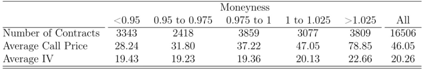
Table I displays the number of contracts, the average call price and the average im-plied volatility across moneyness (Panel (a)), across maturity (Panel (b)), and a detailed cross-tabulation across moneyness and maturity (Panel (c)). The Black-Scholes IV curve is asymmetric in the overall sample, displaying a rising pattern with moneynesss, and signaling a sharp left skew in the risk-neutral distribution of returns. Also, the level of the curve is flat, or slightly decreasing, with maturity. Disaggregation reveals variations in the shape of the IV curve at different maturities. Starting from the shortest maturity, the IV curve initially follows an asymmetric smile with higher volatility values for in-the-money options. Hereafter, the asymmetry increases as we consider longer maturities and the (average) IV curve eventually becomes monotone in moneyness for the longer maturities.
Note that the composition of the sample varies with maturities. Out-of-the-money con-tracts dominate for long maturities while in-the-money concon-tracts dominate for short maturi-ties. This is due to the issuance pattern of new option contracts. Newly issued, long-maturity options are typically deep-out-the-money, in anticipation of the index upward drift through time. As we consider shorter maturities, the composition becomes more balanced. At the shortest horizon, most options are deep in-the-money, since the exchange does not regularly issue short horizon out-of-the-money options. This implies that the average IV curve re-flects, in part, a composition bias with most in-the-money options having short maturities and most out-of-the-money options having long maturities. Because short maturity options
have higher implied volatility on average, this makes the average IV curve more smirked.13
10These subperiods have varying length depending on the (calendar) months they cover.
11Take any contract, on any observation date. This contract is assigned to the 1-month maturity group
if its settlement date occurs on the following third-Friday, to the 2-month group if it occurs on the next to following third-Friday, etc.
12Within a given month, and within a given maturity group, the same contract (i.e. same strike price)
is observed with successively shorter maturities. However it is priced consistently under the null of i.i.d. returns innovations throughout the month.
13This highlight the importance of using a model which can handle maturity differences. In particular,
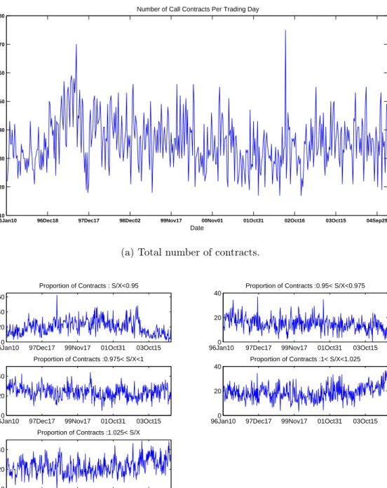
Finally, Panel (a) of Figure 1 presents the number of available observations for each day, which averages around 40 and typically ranges between 20 and 50 contracts. Panel (b) de-composes this number and presents the proportion of contracts in each moneyness category. An ongoing extension of this paper is to include both call and put options and obtain a more balanced sample across moneyness as well as a better coverage of longer maturities.
IV
The Volatility Spread And The Equity Premium
A Model’s Implications
The relationship between skewness and volatility runs deeper than a simple redistribu-tion of probability mass across the support of returns. That is because the impact of the representative investor’s preference on the risk-neutral volatility depends on skewness. In the particular case where the representative SDF can be approximated by the exponential-shift given in Equation 4 we have a tight link between the price of risk, the volatility spread and skewness. After some manipulation of Equation 7, we obtain
ln (St+i/St)−r(i)−ω(ti)=−2
σ∗(i)−σ(i)
α(ti) +σ ∗(i)ε∗
t+i,
for an investment horizon iand where r(i) is the risk-free rate for that horizon andω
t is the
Jensen adjustment term.14 In the following, we test this implication of the HG model and
its ability to capture the volatility spread and the equity premium. We perform regressions of SP500 (log) excess returns on the ratio of the volatility spread to skewness. The key predictions are that the constant should be zero and that coefficients should be -2.
B Aggregating Data
We obtain estimates of risk-neutral volatility and skewness from option data. Estimates of skewness are noisy in weekly data. This is in part due to the number of option prices available each week and, also, to the sampling frequency. One simple solution is to group price observations at the monthly level where we define a month as the period between successive expiration dates which occur every third Friday (See Section III). Within each month, the data consists of repeated observations of the same contracts over a period of 4
(or 5) weeks.15 This implicitly assumes i.i.d. return innovations throughout a month, which
14This term is a function of both skewness and volatility but the first term of its Taylor expansion is the
usual correction in the Gaussian case, 1
2σ2.
15Some contracts are not observed each Wednesday within a month. New contracts become available
is consistent with the model and reasonable over this short time span. It also implies that
the maturity date of each contract is constant throughout each month and, thus, that the
skewness estimate pertains to a set of contracts that mature at fixed maturities. Finally, we measure the historical volatility using the observed realized volatility.
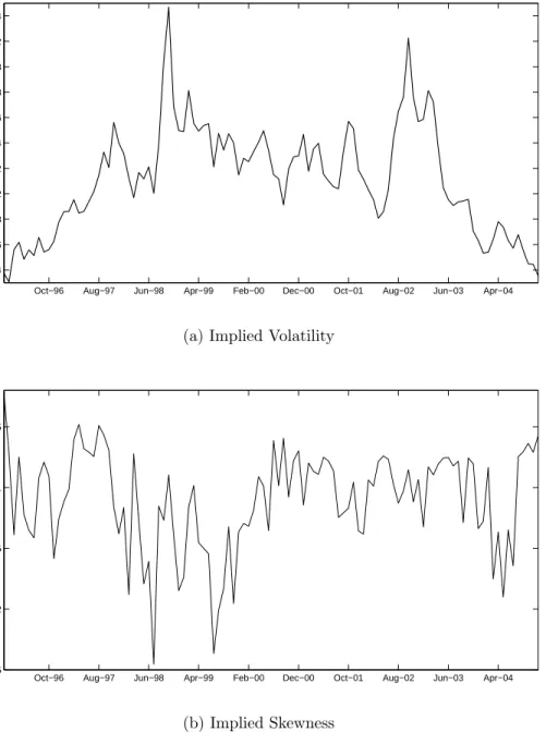
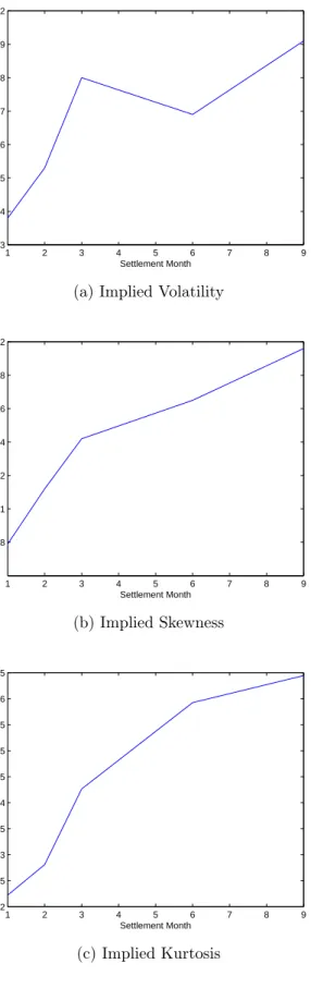
We estimate our preferred version of the model each month through minimization of
squared pricing errors.16Figure 2 presents the time series of our volatility estimates (Panel (a))
and of our skewness estimates (Panel (b)). Skewness typically varies around -1 but dipped close to -2.5 in the summer of 1998 and in the second half of 1999, and slightly below 1.5 in the Fall of 1996 and the Spring of 2004.
C Implied Skewness And The Risk Premia
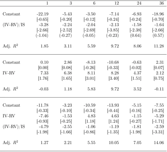
Table II presents the results from regressions of excess returns at horizons of 1, 3, 6,
12, 24 and 36 months on the ratio of the volatility spread to skewness. 17 The results are
striking. Point estimates for the slope coefficient are close to -2 as predicted by the model. Moreover, at horizons of 3, 6, and 12 months, where we would expect the forward-looking nature of the option-implied estimate to be the most relevant, estimates are -2.24, -2.04 and -2.13, respectively. In fact, at any horizon, we cannot reject the null hypothesis that the coefficient is equal to -2. Next, the constant is not significantly different from zero so that the two most important implications of the model cannot be rejected empirically. Finally,
the predictability of excess returns is low at the 1-month horizon (i.e.R2 is 1.85%) but rises
steadily with the horizon, reaching 5.6%, 9.7% and 11.3% at horizons of 6, 12 and 36 months. For comparison with results available in the existing literature, we also consider regres-sions on the volatility spread which displays some predictive power at horizons of 9 and 12 months. However, coefficients are not significant at other horizons. Finally, we ask if the volatility spread contains information beyond that revealed by the volatility to skewness ra-tio. The results from the regressions are presented in Table II. Since volatility and the ratio of the volatility spread to skewness are highly correlated, the coefficients become unreliable, even changing signs in many cases for the volatility spread. However, their combined pre-dictive power does not rise above that of the volatility to skewness ratio, further supporting the implications of the model.
available each week because they were excluded from the weekly sample due to liquidity concerns.
16Specifically, we estimate a restricted version of the practitioner’s HG model that allow for kurtosis but
maintain the identification of the risk-neutral volatility and skewness (See Section VII). As a robustness check (not reported) we repeated the exercise using skewness estimated from the simple HG model presented above. The results are not qualitatively different.
17Precisely, our measures of risk-neutral moments pertain only to the distribution of returns at a horizons
of 12 months or less. Nonetheless, if these moments exhibit persistence, their predictive power will extend to longer horizons as is indeed the case
D Discussion
We can also interpret the results in the broader context of a general equilibrium model. There, the price of risk is determined by preference parameters. In particular, in an economy
with power utility,νcorresponds to the risk-aversion parameter (see e.g. Bakshi et al. (2003))
which can be estimated given estimates of the risk premium, µ−r, and return volatility,σ,
obtained from observed returns data. Equation 6, which is repeated here,
ν+1 2 ≈ µ−r σ2 + 1 2 (µ−r)2 +σ4 12 σ3 α ∗,
shows that ignoring skewness (the last term) leads to upward bias in the estimate of the price of risk and, hence, of risk aversion. Intuitively, when agents are risk-averse, and the risk premium is positive, a more negative value of skewness corresponds to an increase in the quantity of risk: the probability of lower returns increases. Then accounting for skewness reduces the price of risk required to fit the observed equity premium and, ultimately, leads to lower, unbiased, estimates of risk aversion in the economy.
Note that the effect of skewness is economically significant. Since 1980, the sample mean and volatility of one-year returns is 14.72% and 6.13%, respectively, and the first term of Equation 6 is equal to 20.5. In other words, if risk is summarized by the volatility of market returns, then the equity premium appears too large and leads to excessively high estimates
of the coefficient of risk aversion. However, the coefficient of skewness, α, in the last term
is 12.88. For a value of skewness, say, of -1, the estimate of the price of risk is 7.63, less than half than if we ignore the impact of skewness. Moreover, the estimates of skewness we obtain below are often lower than -1.
The results shows the linkages implied by the HG model between the equity premium, the volatility spread and the skewness hold (Equation 7). This suggests that an understanding of the volatility spread and of the equity premium demands an understanding of the deter-minants of risk-neutral skewness. Moreover, it shows that properly conditioning on implied skewness is key to deciphering the information content of options prices for future returns. Recall that in this model the volatility spread is due to the presence of skewness. In fact, reversing the relationship, and interpreting the volatility spread as the returns on a specific portfolio of options, p h∗ t − p ht= 1 2α∗ t ³ EP t [ln (St+i/St)]−EtQ[ln (St+i/St)] ´
the volatility spread portfolio. This offers a solution to the question posed in Carr and Wu (2008) which asks what factor may explain the volatility spread.
Our results contrast with existing results (e.g. Bakshi and Kapadia (2003), Bollerslev et al. (2008)) where the spread is linked to variance risk being priced. In our model, the
asymmetry in returns shifts the price of riskand the risk-neutral volatility. This induces the
link between the volatility spread and the equity premium. Similarly, Polimenis (2006) and
Bakshi and Madan (2006) link the volatility spread to higher order moments of thehistorical
distribution. In particular, Bakshi and Madan (2006) conclude that the historical skewness plays a relatively small role in the determination of volatility spread. They did not consider neutral skewness. One important implication is that understanding the source of risk-neutral skewness is a key research objective. From the tight linkages we uncover, we conclude that an understanding of the volatility spread, and its relationship with the compensation for risk, demands an understanding of risk-neutral skewness. In particular, this new stylized fact should help discriminate across competing theories of the observed volatility spread.
Finally, one drawback is that mis-specification of the parametric model affects the results through a measurement errors problem. In an ongoing extension of the paper, we check the robustness of the results to the use of non-parametric measures and increase the efficiency of the test through GLS regressions.
V
Implied Volatility and Skewness Surface
In the context of the BSM model, it was recognized early that inverting option prices for the volatility parameter provided a good measure of future returns volatility. However, the HG model offers a separate parametrization for volatility and skewness. This allows us to easily measure both the volatility and skewness implicit in option prices. This is important because while alternative parametric (e.g. ARCH) and non-parametric (e.g. Realized Volatility)
measures of volatility exist18, the lack of robustness of the usual sample skewness estimator
is well known (e.g. Kim and White (2003)).
In this section, we study the trade-offs involved between volatility and skewness when fitting option prices. We first analyze how the implied volatility curve varies across different values of skewness and, second, how the implied skewness curve varies with volatility. The results are intuitive. The impact of skewness on implied volatility is asymmetric, depending both on the sign of skewness and of moneyness. In particular, negative skewness tilt a
18See Bates (1995) for a review of the literature on the forecasting of volatility using option prices and
smirked IV curve toward a symmetric smile. On the other hand, the impact of volatility on implied skewness displays a more complex pattern.
An important conclusion from this section is that the HG model exhibits enough flexibility to restore the symmetry of the volatility smile. Moreover, the level of implied volatility or, alternatively, the implied volatility of at-the-money options is sensitive to the choice of the skewness parameter. In particular, this implies that empirical studies of the volatility spread are based on BSM implied volatility are affected by measurement errors due to the impact of skewness.
A Inverting The Implied Volatility and Skewness Surface
Volatility and skewness cannot be inverted uniquely from a single option price. Instead, for each strike price, the HG model implies a function describing the set of volatility and skewness pairs matching the observed price: a volatility-skewness curve. This is in contrast with the BSM model where any given option price can be inverted uniquely for the volatility parameter. Of course, if the HG model is true, using options with different strike prices would identify uniquely a volatility-skewness couple. In fact, only two different strike prices would be sufficient for this purpose. In practice, the HG model extends the BSM model in only one direction, allowing for a skewness parameter. Other deviations from the underlying assumptions cause the volatility-skewness curve to vary across moneyness in such a way that no unique couple can match every observed price. Thus, in the HG model, the counterpart to
the IV curve is the implied volatility and skewnesssurface. This surface is the representation
of the set of volatility and skewness pairs matching the observed option prices for varying strike prices.
To draw the volatility and skewness surface, we first pick a value of skewness from a grid. Then, each day and for each available strike price, we invert the option price for the volatility parameter and obtain an implied volatility curve. As we vary the value of skewness we obtain different IV curves and, altogether, they yield an implied volatility and skewness surface. A section of this surface at a given value of skewness is one possible IV curve. Each day, these different IV curves are alternative, and equivalent, representations of the data. Each embodies all the information about the distribution of returns and, in addition, measurement errors due to transaction costs, illiquidity and asynchronous trading. Below we analyze the results within each maturity category, and in the aggregate.
B Impact Of Skewness on Implied Volatility Curves
This section traces the average implied volatility and skewness surface across time and maturity groups. This provides a smoother picture of the impact of skewness on the IV
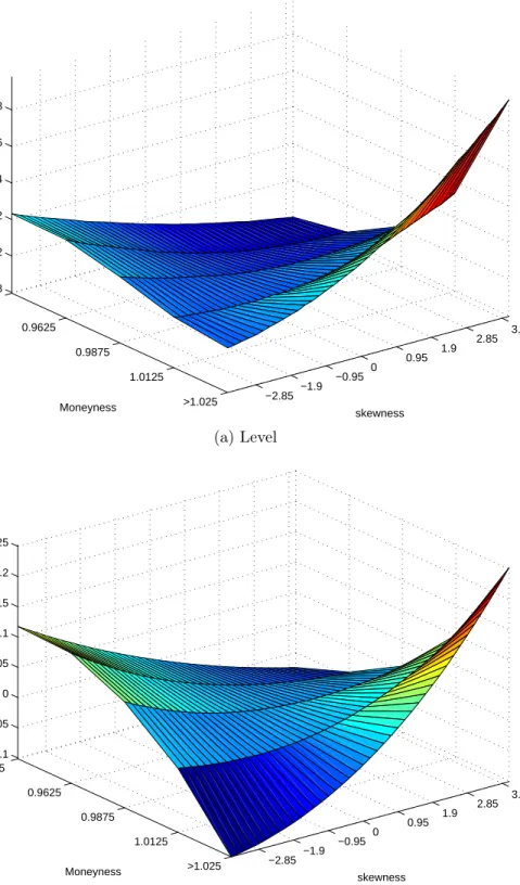
curve. The average volatility-skewness surface is given in Figure 3 in level (Panel (a)) and in percentage deviations from the the benchmark BSM IV curve (Panel (b)). Panel (a) display the usual smirk in the IV curve when skewness is zero. More interestingly, it shows
that the average IV curve is flat for values of skewness around -1.19 Clearly, the HG model
is sufficiently flexible to capture the skewness implicit in option prices. Next, consider the deviations from the BSM curve in Panel (b). The case with skewness equal to zero corresponds to a straight line at zero. As we consider values of skewness away from zero, the IV curve is tilted one way or another depending on the sign of return asymmetry considered. For negative values of skewness, the IV curve is tilted toward positive value of moneyness. Conversely, for positive values of skewness, the IV curve is tilted toward negative values of moneyness. In other words, as we shift probability mass toward the left (right) tail of the return distribution, the implied volatilities required to match observed prices increase (decrease) for out-of-the-money calls and decreases (increases) for in-the-money calls thereby tilting the IV curve back toward a symmetric smile. In the extreme cases, allowing for non-zero skewness can raise or decrease measured implied volatility by more than 15% relative to the BSM case.
C Results For Different Option Maturities
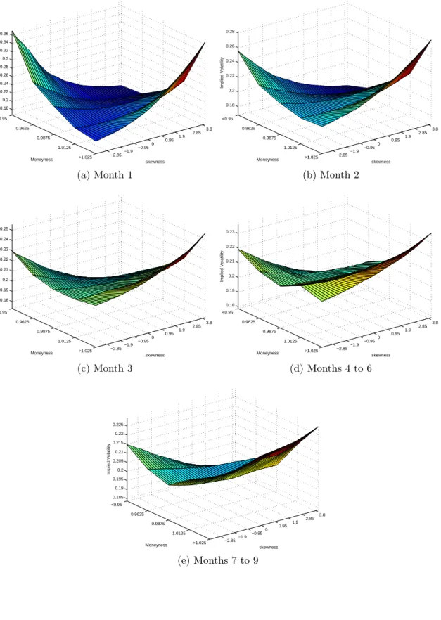
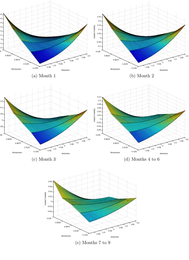
Next, Figures 4(a)-(e) present implied volatility and skewness surfaces within different maturity groups while Figures 5(a)-(e) report the same results but in percentage deviations from BSM values. Note first that when skewness is zero, which corresponds to the BSM case, we observe sharp differences between implied surfaces at different maturities. As discussed in section III, the average BSM IV curve is a slightly asymmetric smile for short maturities: implied volatility obtained from in-the-money options is higher than for out-of-the-money options. The smile then gradually disappears as we increase maturity and the IV curve eventually becomes smirked. For negative values of skewness, and for any maturity, the IV curve is tilted toward a symmetric smile. For contracts maturing at the next settlement date, small negative values of skewness appears sufficient to establish a symmetric smile. As we increase maturity, however, more negative values are necessary. Looking at Figure 5 we see that the impact of a given variation in skewness is much lower for the longest maturity.
D Impact Of Volatility On Implied Skewness
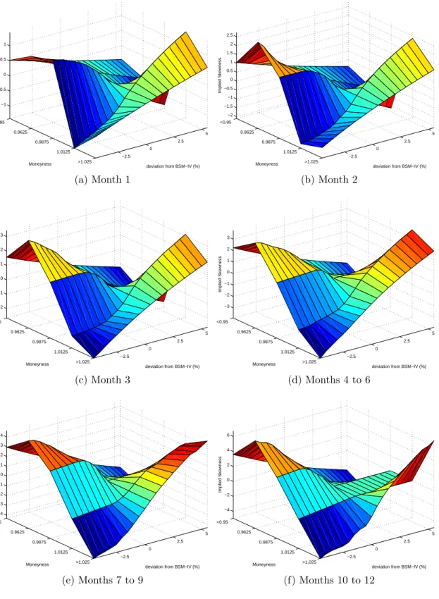
Figures 6(a)-(f) present implied values for skewness across different values of implied volatility. For at-the-money options, there is no tradeoff between volatility and skewness.
19The curve is not strictly flat and this may be due to the impact of kurtosis, or to a composition effect.
However, the impact of volatility on implied skewness is asymmetric and highly nonlinear on both side of the moneyness spectrum. As the volatility of returns decreases, and the probability mass is closer to the mean, the skewness value required to match observed price increases for out-of-the-money options, implying a higher right-tail, but decreases for in-the-money options, implying a lower left-tail. The reverse is true when we increase the value of volatility. In both cases the impact is not monotonic as we move away from at-the-money. Rather, the pattern follows a sharp V-shape, or inverted V-shape, where changes of volatility have no impact on implied skewness for at-the-money options, the largest impact for intermediate moneyness, a lower impact for distant moneyness. This is likely an indication of a trade-off between the skewness and the kurtosis in the HG distribution to match observed prices. Finally, the impact of volatility on implied skewness rises with the option maturity.
VI
Practitioner’s Models
The previous section shows that the implied volatility and skewness surface can be described as the smooth tilting of the IV curve across values of skewness. However, while the HG model provides enough flexibility to match the skewness present in option data, the IV curve
typically remains slightly curved. This is may due to excess kurtosis.20 In this section, we
introduce the practitioner’s variants of the BSM model BSM] and of the HG model [P-HG]. These capture deviations from risk-neutral distributions by modeling volatility as a quadratic function of moneyness. That is, in the P-BSM case,
σ(ξ) = σI0(α, κ)(1 +γ1(α, κ)ξ+γ2(α, κ)ξ2)
where ξ is moneyness and α and κ are the skewness and excess kurtosis of the risk-neutral
distribution. Note that σ(0) = σI0 and that moneyness is defined as
ξ= ln(S/K)(−rτ) ¯
σ√τ ,
to correct for maturity differences where S, K, τ and σ¯ denote the stock price, the strike
price, the time to maturity and the average implied volatility, respectively.
In the following, we first document that estimates of sigmaI0, γ1, and γ2 vary when
we allow for skewness. This contrast with the usual interpretation of γ1 as a measure of
skewness. Next we show that the P-HG model is justified as an expansion around the HG
20In contrast with the Gaussian case, the kurtosis of the HG distribution varies with parameter values.
density. This results is the analog of the justification of the P-BSM model as an expansion around the Gaussian density. However, we provide restrictions on parameters of the IV
function such that we can recover estimates of α and κ.
A Unconstrained IV Curves
The practitioner’s IV curve smooths through the cross-section of option prices, ignores local idiosyncracies and focuses on the impact of higher-order moments. This approach is
pervasive because of its empirical performance and, also, because its parameters (i.e. σI0, γ1
and γ2) are usually interpreted in terms of the variance, skewness and kurtosis of the true
underlying risk-neutral distribution.21 Zhang and Xiang (2005) argue that in the Gaussian
case and up to a first-order approximation σI0(β, κ) is linear in the risk-neutral volatility,
γ1(β, κ) is linear in skewness, and γ2(β, κ) is linear in kurtosis. For these reasons, the
coefficients of the IV function are usually left unrestricted at estimation.
To evaluate empirically the impact of skewness on estimated IV curves, we fix the value of
βand estimate the P-HG model at each date by minimizing squared pricing errors. We repeat
the exercise for different values of skewness. We then average unconstrained estimates of
σI0,t, γ1,t and γ2,t through time and trace their relationship with skewness. Figure 7 presents
the results. Panel (a) presents average estimates ofσI0. For contracts maturing at the next
settlement date, at-the-money implied volatility is 20% on average when skewness is zero. When (absolute) skewness increases, estimates of at-the-value volatility increases as high as 23%. Intuitively, shifting some probability mass toward one side involves a trade-off for pricing in-the-money versus out-the-money options. For a constant level of skewness, this tension can be reduced by an increase in the level of volatility. A similar pattern occurs at longer maturities, but the impact of skewness gradually decreases. Panel (b) presents the
results for the asymmetry parameter. In line with intuition we find that γˆ1 varies linearly
with the value of β : both parameters are measures of the underlying skewness. Finally,
Panel 8c shows that γˆ2 also varies (non-linearly) substantially with skewness.22 For each
parameter, the variations with skewness are stronger for shorter maturities.
The strong dependence between the skewness and all parameters of the IV curve implies that information on the underlying risk-neutral moments is shared across parameters.
Fur-thermore, the fact that estimates of β and of γ1 are (linearly) correlated implies that they
21σI
0 controls the level of the curve,γ1(β, κ)controls the asymmetry of the curve andγ2(β, κ)controls its
steepness.
22This contrasts with the theoretical results of Zhang and Xiang (2005). However, they assume that the
skewness and excess kurtosis of the underlying distribution can be chosen independently while in fact there is a tight link between the two for any given correctly specified density. Moreover, their linearization strategy may lead to a poor approximation (see below).
are poorly identified. For our purposes, we need to find restrictions on σI0, γ1 and γ2 such
that only βˆ can capture the risk-neutral skewness. Absent these restrictions, parameters
of the IV curve capture some of the asymmetry in the underlying distribution leading to
biased estimates of β. Note that merely imposing γ1 = 0 does not identify an estimator of
β with skewness. The following section introduces a framework which will ultimately lead
us to the desired restrictions. Under these restrictions, any deviation from a flat IV curve
can only be linked to deviations of κ. This sharp identification of parameters in term of the
underlying moments is useful to understand the relative importance of skewness and kurtosis in matching observed prices. More importantly, the unambiguous identification of skewness is necessary to provide a measure of the risk premia from implied volatility and skewness.
B HG Model With Excess Kurtosis
We now provide a rigorous justification of the P-HG model when the true distribution displays excess kurtosis. We can characterize sufficient restrictions on the parameters of the
IV curve such that βˆ is identified as the risk-neutral skewness in this more general model
as well. In this context, parameters of the IV curve are restricted to (known) functions of excess kurtosis. As a by-product, we obtain an estimator of the kurtosis in excess of the Gamma distribution.
We assume that the true density of returns can be represented by an Edgeworth expan-sion around the Gamma distribution. This is similar to earlier work using the Gaussian distribution (Jarrow and Rudd (1982), Corrado and Su (1996)) but the Gamma distribution allows an exact match of the first three moments. We then impose the equality of the option pricing formula under the true model and the P-HG model for at-the-money options.
Suppose that the true evolution of stock returns under the risk neutral measure can be described as
RT = (r−δ∗)T +σ∗
√ T y,
where δ∗ is a risk-adjustment term, y is a random variable with mean zero, unit variance,
skewness, 2√β∗
T and kurtosis, λ
∗
2. If y is normally distributed, then δ = σ
∗2
2 . We allow for
non-normality beyond the HG and assume that the probability density of y is given by
f(y) =g(y) + λ ∗ 2−6β ∗2 T 4! d4g(y) dy4 , (13)
where g(y) is the standardized gamma density. This is a one-term Edgeworth expansion
around the standardized gamma distribution. This approach captures fat tails in excess of the Gamma distribution but ignores deviations beyond the fourth moment. Our objective
here is to allow for non-trivial implied volatility and skewness surface due to excess kurtosis
and derive explicitly the function σI0(κ), γ1(κ) and γ2(κ). Proposition 4 builds on a
no-arbitrage argument and provides a closed-form characterization of option prices and of the risk-adjustment term.
Proposition 4. If the logarithm of gross stock returns has the density given by Equation 13, then the price of a call option, C∗(K, T), with maturity T, underlying price S
0 and strike price K is C∗(K, T) = S0P (a∗, d∗1)−e−rT ¡ 1 +T2σ∗4κ4 ¢ KP(a∗, d∗2) +κe−rTKT2σ∗ β∗3 £ −h00(d∗ 2) +σ∗β∗h0(d∗2)−σ∗2β∗2h(d∗2) ¤ , when β <0 and C∗(K, T) = S 0Q(a∗, d∗1)−e−rT ¡ 1 +T2σ∗4κ 4 ¢ KQ(a∗, d∗ 2) − κe−rTKT2σ∗ β∗3 £ −h00(d∗ 2) +σ∗β∗h0(d∗2)−σ∗2β∗2h(d∗2) ¤ ,
when β >0. We define the excess kurtosis, κ= λ2−6β
∗2 T 4! , and d∗ 2 = ln(K/S0)− h r+ln(1β−2σβ) i T + ln(1 +T2σ4κ) σβ d∗ 1 = d2(1−σβ) a∗ = T β2,
where h is the density of the standard gamma distribution.
C Identified practitioner’s HG
We are now looking for the restrictions on the parameters of the P-HG model such that
estimation of β delivers a convergent estimate of the risk-neutral skewness β∗. Zhang and
Xiang (2005) provide the restriction for the case where the Gaussian density is used in the approximation. To find the link between the parameters of the P-HG model with parameters
of the true distribution, we impose the following restrictions C∗(K, T) = C(K, T) ∂C∗(K, T) ∂K = ∂C(K, T) ∂K ∂2C∗(K, T) ∂K2 = ∂2C(K, T) ∂K2
when evaluated at-the-money (i.e.K =S0erT). These restrictions are given in the appendix
but note that they are trivially satisfied whenever κ= 0 since in this case the HG model is
true and the implied volatility-surface is flat. Of course this corresponds to the caseσI0 =σ,
β = β∗ and γ
1 = γ2 = 0. We linearize the restrictions around this point (i.e. κ = 0) and
obtain σI0−σ σ =A1(σ, β)κ (14) γ1 =B1(σ, β) σI0−σ σ +B2(σ, β)κ (15) γ2 =C1(σ, β) σI0−σ σ +C2(σ, β)γ1+C3(σ, β)κ, (16)
where the coefficients are given in the appendix.23 Then, small deviations of the underlying
density from a HG distribution leads to deviations from a flat implied volatility and skewness surface. This highlights the impact of excess kurtosis on the estimates of at-the-money
implied volatility, of γ1 and of γ2. It also makes clear that deviations from a flat implied
volatility and skewness surface are only due to deviations of excess kurtosis from zero. Also, up to a first order, the impact of excess kurtosis on at-the-money implied volatility feedbacks
on estimates ofγ1 and γ2. More importantly, these restrictions ensure thatβ corresponds to
the risk-neutral skewness and that the practitioner’s HG model conforms to the true returns density.
VII
Option Pricing Results
In this section, we estimate each model and compare their performance. The results show that the HG framework substantially improves in-sample, hedging and out-of-sample per-formance. The improvements are robust if we impose the identification of the skewness parameters, as discussed in the previous section. Indeed, the improvements remain when
23We differ from Zhang and Xiang (2005) who linearize the restrictions around σ = 0. Arguably,
lin-earizing around the HG distribution is likely to provide a better approximation than linlin-earizing around the deterministic case.
the only deviation from the simple HG model is a constant adjustment to kurtosis through time. In other words, a fixed implied volatility and skewness surface combined with varia-tions in skewness is sufficient. Overall, our approach delivers a reliable measure of skewness while offering improved forecasting and hedging performance. In contrast, the P-BSM model does not allow for sufficient flexibility to match the skewness implicit in the data and offers lower hedging and out-of-sample performance.
We evaluate the basic HG model as well as three different versions of the P-HG model:
P-HG1, P-HG2, P-HG3. The first version imposes the simple restriction that γ1 = 0. The
second model, HG2, imposes the restrictions derived in the previous section. Finally, P-HG3 is unrestricted. We also introduce a “smoothed” versions of these models where some parameters of the IV curves are held constant through the sample. First, the smoothed
version of the P-HG1 model, labeled SP-HG1, still imposes that γ1 is zero but also holds γ2
constant through time. Next, SP-HG2 still imposes that all deviations from a flat IV curve
are linked to the value of κ but the latter is held constant through time. Finally, SP-HG3
imposes the following structure on the IV curve,
σt(ξ) = σI0,t(1 + (γ10+γ11βt)ξ+ (γ20+γ21βt)ξ2).
which is a simple attempt to implement the observation made in Section VI that parameters of the IV curve vary with skewness. Finally, estimation is performed through minimization of squared pricing errors in the weekly sample.
A In-Sample RMSE
A.1 HG And BSM Models
Table III presents in-sample Root Mean Squared Errors [RMSE] where each results is expressed as a percentage of the BSM’s RMSE. Panel (a) presents results across moneyness while Panel (b) presents results across maturities. Although the most flexible (i.e. P-HG3) model achieves an RMSE which is 14% of the benchmark, most of the improvement comes from using the HG distribution: the simpler HG model’s RMSE is 37%. Of course, this is simply a reflection returns begin non-Gaussian, as reported elsewhere in the literature.
A.2 Practitioner’s Variants
Interestingly, even with one extra parameter, the P-BSM does not offer much improve-ment (35% vs 37%) over the straightforward HG model. The models offer similar results across maturities but their performances differ across strike prices. The P-BSM improves pricing for in-the-money options at the expense of larger errors for other moneyness groups.
On the other hand, the P-HG1 and the P-HG2 models achieve RMSEs that are 28% and 23%, respectively, but no increase in the number of parameters. Moreover, in contrast with the P-BSM model, the lower errors for out-of-the-money options are not compensated by higher errors for options that are nearer the money. Thus, models based on the HG distribution appear to offer more flexibility in choosing risk-neutral skewness and kurtosis.
Next, although the naive γ1 = 0 restriction may seem reasonable, it fails in practice
by yielding larger RMSEs. Comparing models, we see that the improvement of the P-HG2 over the P-HG1 is substantial and is obtained in short maturity, out-of-the-money options. Finally, with one more parameter, the P-H3 offers much lower in-sample RSME (14%) than any other model and yields substantial improvements across all moneyness and maturity categories.
A.3 Smoothed Coefficients
As expected, the various smoothed models yield lower in-sample performance, although note that the SP-HG2 model still improves (31%) over the P-BSM model. These models retain the variability of the skewness parameters from date to date but impose a constant shape on the IV curve through the sample. Overall their performance suggests that time-variation in the shape of the IV curve may be important in-sample. However, out-of-sample results in the next section show that this result is not robust out-of-sample, indicating a relatively minor role for information beyond the third moment.
B Out-of-sample RMSE
The good performance of models based on the HG distribution could be due to over-fitting and might not hold out-of-sample. To check this, we perform the following out-of-sample exercise. First, we estimate each model’s parameter from options in a given week. We then fix these parameters and evaluate the model’s ability to price options observed in the following week. Table IV presents RMSE for each model across strike prices (Panel (a)) and across maturities (Panel (b)).
The relative out-of-sample RMSE increases for all model. This indicates that some of the deviations from the Gaussian case are transitory. The lowest RMSE is now 57%, obtained for the P-HG3 model, while the worst result is 68%, obtained for the P-BSM model. Moreover, keeping the shape of the IV curve constant (i.e. SP-BSM model) offers similar results (67%). This is another piece of evidence that the practitioner’s version of the BSM model does not properly fit the (persistent) skewness and kurtosis present in the data. On-the-other hand, for the purpose of measuring risk-neutral skewness, the performance of the P-HG2 (66%) model is promising.
Strikingly, the SP-HG2 model, which fixes excess kurtosis through the sample, actually improves out-of-sample RMSE (64%) over its the more flexible HG2. Although the P-HG2 model is more flexible, it induces large sample errors for short-maturity, out-of-the-money options. Some of the variations in excess kurtosis required to match (in-sample) option prices in this category seem to be transitory, degrading the out-of-sample performance of the model. A similar remark holds for the P-BSM model. Most of the variations in the shape of the IV curve do not translate into improved out-of-sample pricing. The models differ because in the HG framework we know how to restrict unnecessary variation in kurtosis while retaining the flexibility in skewness. Finally, the P-HG3 model remains the best performer out-of-sample.
C Hedging Errors
Hedging errors implied by each model may convey more economic significance to risk-managers. Below, we verify that allowing for skewness significantly alter hedging strategy theoretically, and improves hedging results empirically. Also, we verify that any improved hedging performance persists at horizons beyond one week. Again, we find that the un-restricted P-HG3 model performs the best. However, the SP-HG2 model, where skewness is separately identified, offers the next best performance, highlighting, again, the value of theoretically sound restrictions.
C.1 Comparing The Greeks
As in the BSM model, we can compute explicitly the sensitivity of option prices to changes in the underlying parameters, including the sensitivity to changes in skewness. We provide these in the appendix. These derivatives depend on the direction of asymmetry and
everywhere the symmetric case (i.e. β = 0) leads to the standard results from BSM.
To see the impact of skewness, we draw options sensitivities across strike prices for different values of skewness. In the computations, we use the average values of volatility, of the interest rate and of the index level. Figure 8 presents results for the first and second derivatives with respect to the underlying, Delta and Gamma, as well as the derivative with respect to volatility, Vega. The results are reported in levels in the top panels (Panel (a) to (c)) and in percentage deviations from the symmetric case in the bottom panels (Panel (d) to (f)). First, the pattern of Delta across moneyness is familiar. The sensitivity is small for deep out-of-the-money options but grows to close to one for deep in-the-money options. Varying skewness does not alter this picture but looking at levels hides significant deviations: at skewness equal to -2.5, which occurs in our sample, short positions in the stock are as much as 20% higher for some out-of-the money options. Also, the sensitivity of Delta to skewness
is large for strike prices that are near the money. Next, the impact on Gamma is dramatic. In the symmetric case, Gamma appears quadratic in moneyness with highest values for at-the-money options. Decreasing skewness lowers Gamma for in-the-money options but increases Gamma for out-of-the-money options. When skewness is -2.5, Gamma becomes monotonous in the strike price and as much as 50% lower then when skewness is zero for in-the-money options and 50% higher for out-of-the-money options. Finally, skewness has a similar, asymmetric impact on the sensitivity of options to variations in volatility. When skewness is -2.5, Vega decreases by more than 20% for out-of-the-money options and increases by nearly 20% for in-the-money options.
Clearly, ignoring the impact of skewness can leads to large hedging errors. The results below will confirm this. Even though the Practiotioners’ BSM [P-BSM] can in principle capture some of the risk-neutral skewness implicit in option prices, either its lack of flexibility, or its inability to identify the separate impact of skewness leads to substantially larger hedging errors.
C.2 Comparing Hedging Performance
We follow Dumas et al. (1998) and compute hedging errors as
²t = ∆Ct,tactual+h −∆Ct,tmodel+h
which is a measure of the impact of changes in model errors from t tot+h on the hedging
strategy.24 Table V and Table VI present the results for hedging horizons from one to four
weeks ahead (i.e. h= 1,2,3,4).
Consider hedging errors at the 1-week horizon (Table Va). First, although the BSM model appears to perform well, its overall mean hedging errors averaging 1.6 cents, this hides important disparities across maturities with average hedging errors ranging from 36.7 cents for out-of-the-mon